Publisher’s version / Version de l'éditeur:
Vous avez des questions? Nous pouvons vous aider. Pour communiquer directement avec un auteur, consultez la
première page de la revue dans laquelle son article a été publié afin de trouver ses coordonnées. Si vous n’arrivez pas à les repérer, communiquez avec nous à [email protected].
Questions? Contact the NRC Publications Archive team at
[email protected]. If you wish to email the authors directly, please see the first page of the publication for their contact information.
https://publications-cnrc.canada.ca/fra/droits
L’accès à ce site Web et l’utilisation de son contenu sont assujettis aux conditions présentées dans le site LISEZ CES CONDITIONS ATTENTIVEMENT AVANT D’UTILISER CE SITE WEB.
Research Report (National Research Council of Canada. Institute for Research in Construction), 2008-09-12
READ THESE TERMS AND CONDITIONS CAREFULLY BEFORE USING THIS WEBSITE. https://nrc-publications.canada.ca/eng/copyright
NRC Publications Archive Record / Notice des Archives des publications du CNRC :
https://nrc-publications.canada.ca/eng/view/object/?id=29ad5611-93bd-4d84-b5c4-0145de281b96 https://publications-cnrc.canada.ca/fra/voir/objet/?id=29ad5611-93bd-4d84-b5c4-0145de281b96
NRC Publications Archive
Archives des publications du CNRC
For the publisher’s version, please access the DOI link below./ Pour consulter la version de l’éditeur, utilisez le lien DOI ci-dessous.
https://doi.org/10.4224/20373911
Access and use of this website and the material on it are subject to the Terms and Conditions set forth at
International Road Tunnel Fire Detection Research Project - Phase II Task 3: Computer Modelling
Kashef, A.; Ko, S. K. P.; Hadjisophocleous, G. V.; Liu, Z. G.; Lougheed, G. D.; Crampton, G. P.
http://irc.nrc-cnrc.gc.ca
I nt e r nat iona l Roa d Tunne l Fire
De t e c t ion Re se a rch Proje c t -
Pha se I I Ta sk 3 : Com put e r
M ode lling
R R - 2 7 1
K a s h e f , A . ; K o , K . P . ; H a d j i s o p h o c l e o u s , G . V . ; L i u , Z . G . ; L o u g h e e d , G . D . ; C r a m p t o n , G . P .Sept. 12, 2008
The material in this document is covered by the provisions of the Copyright Act, by Canadian laws, policies, regulations and international agreements. Such provisions serve to identify the information source and, in specific instances, to prohibit reproduction of materials without written permission. For more information visit http://laws.justice.gc.ca/en/showtdm/cs/C-42
Les renseignements dans ce document sont protégés par la Loi sur le droit d'auteur, par les lois, les politiques et les règlements du Canada et des accords internationaux. Ces dispositions permettent d'identifier la source de l'information et, dans certains cas, d'interdire la copie de documents sans permission écrite. Pour obtenir de plus amples renseignements : http://lois.justice.gc.ca/fr/showtdm/cs/C-42
International Road Tunnel Fire Detection Research Project – Phase II
TASK 3: COMPUTER MODELLING
Prepared by
A. Kashef, Y. Ko, G. Hadjisophocleous, Z. G. Liu, G. Lougheed, G. Crampton
Fire Research Program
Institute for Research in Construction
International Road Tunnel Fire Detection Research Project – Phase II
Project Technical Panel
Frank Gallo, Port Authority of New York and New Jersey Harry Capers, New Jersey DOT
Alexandre Debs, Ministry of Transportation of Quebec Jesus Rohena, Federal Highway Administration
Paul Patty, Underwriters Laboratories Inc. Volker Wetzig, Versuchs Stollen Hagerbach AG Art Bendelius, A & G Consultants
Bill Connell, Parsons Brinckerhoff
Margaret Simonson, Swedish National Testing and Research Institute Gary English, Seattle Fire Department
Peter Johnson, ARUP Fire Risk & Security Jim Lake, NFPA staff liaison
Principal Sponsors
Ministry of Transportation of British Columbia Ministry of Transportation of Ontario
Ministry of Transportation of Quebec
The City of Edmonton, Transportation Department, Transit Projects Branch AxonX LLC
Siemens Building Technologies Tyco Fire Products
VisionUSA
Sureland Industrial Fire Safety
United Technologies Research Corporation
Contributing Sponsors
National Research Council of Canada
Port Authority of New York and New Jersey A & G Consultants
PB Foundation Micropack, Inc.
J-Power Systems and Sumitomo Electric U.S.A., Inc. Honeywell Inc.
EXECUTIVE SUMMARY
This report presents the results of Task 3 “Computer Modelling” of the International Road Tunnel Fire Detection Research Project (Phase II). Computational Fluid Dynamics (CFD) numerical simulations were conducted, using the Fire Dynamic Simulator (FDS), to help understand and optimize the technical specifications and installation requirements for application of fire detection technologies in road tunnels.
Twenty CFD simulations were conducted to replicate laboratory and field full-scale experiments. The simulations covered different fire sizes, location, ventilation scenarios, and fuel type. Comparisons of temperature and smoke optical density (OD) were made at different locations corresponding to lab and field measurements points.
Three series of CFD simulations were conducted to compare numerical predictions against selected full-scale fire tests (Tasks 2, 4, and 7 of the project). The comparisons were conducted for non-ventilated and longitudinal ventilation conditions. Two types of fire scenarios were simulated: pool fires (under and behind vehicles) and stationary vehicle fires (engine or passenger compartment), using the same dimensions as used in the full-scale tests. Fire sizes varied from approximately 100 KW to 3,400 kW with various growth rates (1 min to 12 min to reach the maximum heat release rate). The CFD simulations involved various fire locations (underneath a vehicle and behind a large vehicle) and various fuel types (gasoline, propane, wood crib and polyurethane foam).
In general, favourable comparisons between the numerical predictions and experimental data were observed. Discrepancies were noted in some comparisons. Both radiation and turbulence close to the fire source had a significant effect on the numerical predictions at these locations. For large fire sizes and highly turbulent situations, these effects were more pronounced. Away from the fire, the predications and hence the comparison with the experimental results were improved as the effect of both radiation and turbulence was reduced.
The numerical predications fluctuated with large amplitudes especially at locations closer to the fire. The experimental results did not exhibit the same phenomenon. This can be attributed to two reasons: the frequency of data collection was coarse and the plume shape was not properly replicated in the numerical simulation. As the size of the pool fire increased, the instability of flames was more pronounced and hence larger fluctuations were observed.
In some cases where the fire plume was deflected differently than what was observed in the corresponding full-scale test, the vertical profile close to the fire was altered and the maximum plume temperature was shifted up or down depending on the angle of deflection of the plume.
In general, the comparisons were more favourable for the scenario with a fire behind a vehicle than for the case of fire under a vehicle. This can be attributed to the fact that the fire under a vehicle was under-ventilated. In general, FDS is more suited for well-ventilated cases.
Four types of ventilation systems and two tunnel lengths were investigated. The ventilation systems included: longitudinal, full-transverse, semi-transverse (supply), and semi-transverse (exhaust). The two investigated tunnel lengths were 37.5 m and 500 m. The 37.5 length is the same length as the test tunnel facility.
Among the investigated ventilation schemes, the semi-transverse supply ventilation system resulted in the highest ceiling temperature and soot volume fraction. Both the full-transverse and semi-full-transverse exhaust ventilation systems produced similar average ceiling temperature and soot profiles. The longitudinal ventilation system resulted in the lowest average ceiling temperature. The semi-transverse supply ventilation system resulted in the fastest rate of rise of ceiling temperature and the semi-transverse exhaust ventilation system resulted in the slowest rate of rise of ceiling temperature.
The ceiling temperature and soot volume fraction profiles for the two tunnel lengths were very similar implying that the length of the tunnel has limited effect on the ceiling temperature and smoke density.
In certain cases, the ventilation system or the prevailing wind could result in a strong longitudinal airflow in the tunnel causing a significant tilting of fire plume. This could, in turn, result in the shift of the hot spot and sometimes, depending on the strength of the airflow, slow/prevent the formation of a hot layer. In these cases, the performance of detection systems that rely on absolute temperature or rate of temperature rise in detecting a fire incident may be compromised. Moreover, the strong longitudinal airflow may disrupt the structure of the fire plume altering its regular shape. Consequently, it becomes more difficult for detection systems that depend on visualizing the fire flame to detect the fire incident.
The existence of stopped traffic in the tunnel could affect the flow field in the tunnel. It may lead to faster flow in some areas resulting in lower temperatures, or to pockets of stagnant air resulting in higher temperatures. Moreover, it may obstruct the viewing zone of detection systems causing a delay in detecting a fire. Although traffic pattern was not investigated in the current study, the existence of an obstruction can greatly affect the fire dynamics.
In general, the data predicted by the CFD simulations can be related to the performance of spot heat detector, linear heat detection systems, and smoke aspiration detection systems. However, more effort is required to relate CFD data to the video imaging detection (VID) and flame detection systems. CFD can provide temporal and spatial information on the expected shape of the plume (flame envelope), heat flux, wall temperature, which may be useful in linking the simulation results to the performance of optical-based detection system.
ACKNOWLEDGEMENTS
The project is conducted under the auspices of the Fire Protection Research Foundation (FPRF). The authors would like to acknowledge the support of the Technical Panel, Sponsors as well as many NRCC staff to this project. A special acknowledgement is noted to Kathleen Almand of the FPRF for her contribution in organizing the project.
TABLE OF CONTENTS
EXECUTIVE SUMMARY ... 3
1 INTRODUCTION... 9
2 COMPARISONS OF CFD NUMERICAL PREDICTIONS AGAINST FULL-SCALE EXPERIMENTS... 10
2.1 Pre Full-Scale Tests CFD Simulations ... 10
2.2 Post Full-Scale Tests CFD Simulations... 11
2.2.1 Series A... 12
2.2.2 Series B ... 29
2.2.3 Series C ... 40
2.3 Conclusions... 41
3 INVESTIGATION OF THE IMPACT OF DIFFERENT PARAMETERS ON FIRE BEHAVIOR AND DETECTION SYSTEM PERFORMANCE... 56
3.1 Ventilation Systems... 56
3.2 CFD Simulations – Series D ... 56
3.3 CFD Simulations – Series E ... 66
3.4 Effect of Tunnel Length Parameter ... 77
3.5 Conclusions... 82
TABLE OF TABLES
Table 2-1 CFD Simulations (Series A Tests - No ventilation)... 13
Table 2-2 CFD Simulations (Series B Tests - With ventilation)... 31
Table 2-3 CFD Simulations (Series C Viger Tunnel Tests)... 42
Table 3-1 Effect of Ventilation Type (Series D - Fire behind a vehicle)... 58
Table 3-2 Effect of Ventilation Type (Series E - Fire behind a vehicle) ... 68
TABLE OF FIGURES
Figure 2-1 Demonstration Test ... 10Figure 2-2 Predicted HRR ... 10
Figure 2-3 Demonstration test: computational domain, initial and boundary conditions... 11
Figure 2-4 Numerical predictions versus experimental data – Demonstration test ... 12
Figure 2-5 Temperature comparisons - Tun2UV1... 16
Figure 2-6 Temperature comparisons - Tun2UV2... 17
Figure 2-7 Temperature comparisons - Tun2UV3... 18
Figure 2-8 Temperature comparisons - Tun2UV4... 19
Figure 2-9 Temperature comparisons - Tun2BV5... 20
Figure 2-10 Temperature comparisons - Tun2BV6... 21
Figure 2-11 Temperature comparisons - Tun2BV7... 22
Figure 2-12 Temperature comparisons - Tun2BV8... 23
Figure 2-13 Temperature comparisons - Tun2EC9 ... 24
Figure 2-14 Temperature comparisons - Tun2PC10 ... 25
Figure 2-15 Temperature comparisons - Tun2PC11 ... 26
Figure 2-16 Smoke comparisons - Tun2BV5 ... 27
Figure 2-17 Smoke comparisons - Tun2BV8 ... 28
Figure 2-18 Temperature comparisons - Tun2UV21... 32
Figure 2-19 Temperature comparisons - Tun2UV22... 33
Figure 2-20 Temperature comparisons - Tun2UV23... 34
Figure 2-21 Temperature comparisons - Tun2UV24... 35
Figure 2-22 Temperature comparisons - Tun2BV25... 36
Figure 2-23 Temperature comparisons - Tun2BV26... 37
Figure 2-24 Smoke comparisons - Tun2BV22 ... 38
Figure 2-25 Smoke comparisons - Tun2BV25 ... 39
Figure 2-26 Series C – schematic of fire locations and measuring locations ... 43
Figure 2-27 Temperature comparisons – Tun4VF3 (Drop 1)... 44
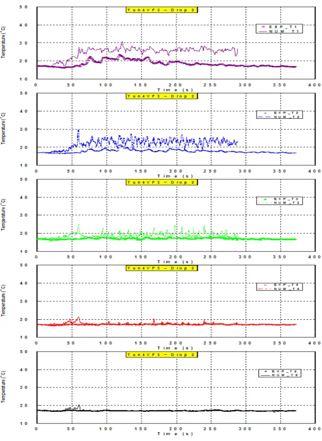
Figure 2-28 Temperature comparisons – Tun4VF3 (Drop 2)... 45
Figure 2-29 Temperature comparisons – Tun4VF3 (Drop 3)... 46
Figure 2-30 Smoke comparisons – Tun4VF3... 47
Figure 2-31 Temperature comparisons – Tun4VF6 (Drop 1)... 48
Figure 2-32 Temperature comparisons – Tun4VF6 (Drop 2)... 49
Figure 2-33 Temperature comparisons – Tun4VF6 (Drop 3)... 50
Figure 2-34 Smoke comparisons – Tun4VF6... 51
Figure 2-35 Temperature comparisons – Tun4VF8 (Drop 1)... 52
Figure 2-37 Temperature comparisons – Tun4VF8 (Drop 3)... 54
Figure 2-38 Smoke comparisons – Tun4VF8... 55
Figure 3-1 Different ventilation systems ... 59
Figure 3-2 Temporal airflow speeds at mid-tunnel section – Series D... 60
Figure 3-3 Temporal airflow temperature predictions at mid-tunnel section – Series D ... 61
Figure 3-4 Average airflow speeds at mid-tunnel section – Series D... 62
Figure 3-5 Average ceiling temperature along the tunnel – Series D... 63
Figure 3-6 Average vertical temperature at mid-tunnel section – Series D... 64
Figure 3-7 Average ceiling soot volume fraction along the tunnel – Series D... 65
Figure 3-8 Different ventilation systems – Series E ... 69
Figure 3-9 Average airflow speeds at mid-tunnel – Series E ... 70
Figure 3-10 Average temperature along the ceiling of tunnel middle portion – Series E ... 71
Figure 3-11 Average airflow temperature at mid-tunnel – Series E... 72
Figure 3-12 Average soot volume fraction along the ceiling of tunnel middle portion – Series E ... 73
Figure 3-13 Smoke and temperature rendering – Series E (Tun2DFT1)... 74
Figure 3-14 Smoke and temperature rendering – Series E (Tun2DNV1) ... 75
Figure 3-15 Smoke and temperature rendering – Series E (Tun2DLT1) ... 76
Figure 3-16 Average airflow speeds at mid-tunnel – Series D & E ... 78
Figure 3-17 Average airflow temperature along the tunnel – Series D & E... 79
Figure 3-18 Average airflow temperature at mid-tunnel – Series D & E... 80
1 INTRODUCTION
A number of technical issues related to the use of current fire detection technologies for road tunnel protection were identified in Phase I of the International Road Tunnel Fire Detection Research Project [1]. This report presents the results of Task 3 “Computer Modelling” of the International Road Tunnel Fire Detection Research Project (Phase II). Computational Fluid Dynamics (CFD) numerical simulations were conducted to help understand and optimize the technical specifications and installation requirements for application of fire detection technologies in road tunnels.
Due to the rapid development of computer technology and huge costs of test programs, the use of CFD models to simulate the dynamics of fire behaviour in tunnels is increasing quickly. The details of fluid flow and heat transfer provided by CFD models can prove vital in analyzing problems involving far-field smoke flow, complex geometries, and impact of fixed ventilation flows.
The work of Task 3 included the following CFD modelling activities: Pre full-scale tests:
o CFD simulations were carried out to compare numerical predictions against the data from a demonstration test in the laboratory tunnel facility to verify the use of FDS for tunnel applications.
o Further simulations were used to assist in the preparation of the full-scale experiments.
Post full-scale tests:
o The numerical predictions were compared against selected experimental data from the laboratory and field experiments.
o Further simulations were used to investigate the impact of different parameters on fire behaviour and detection system performance. These parameters included: fire scenarios, ventilation mode, and tunnel length. Information from the model can be used in developing appropriate test protocols and for understanding and optimizing the performance of fire detection systems used for road tunnel protection.
The current research study employs the Fire Dynamic Simulator (FDS) [2] to study the fire growth and smoke movement in road tunnels. FDS is based on the Large Eddy Simulation (LES) approach and solves a form of high-speed filtered Navier-Stokes equations, valid for low-speed buoyancy driven flow. These equations are discretized in space using second order central differences and in time using an explicit, second order, predictor-corrector scheme.
The initial and boundary conditions of each simulation were set to mimic the conditions of the corresponding test. Comparisons were made to temperature and smoke optical densities measurements.
2 COMPARISONS OF CFD NUMERICAL PREDICTIONS AGAINST
FULL-SCALE EXPERIMENTS
To establish the validity of using the FDS code for the tunnel applications, numerical predictions were compared against selected experimental data from the laboratory and field experiments. The following sections present a sample of these comparisons.
2.1 Pre Full-Scale Tests CFD Simulations
CFD simulations were carried out to compare numerical predictions against the data from a demonstration test conducted in the laboratory tunnel facility to verify the use of FDS for tunnel applications. The tunnel facility is 37.5 m long, 10 m wide and 5.5 m high (Figure 2-1). It can be used for conducting tests that realistically simulate fires in roadway and mass-transit tunnels. The tunnel has two end doors, one large side door to an adjacent burn hall at the West end of the tunnel, and two side louvers at the East end of the tunnel.
Smoke produced in the tunnel facility can be collected and exhausted through a fan system mounted on the test tunnel. For the present work, however, only natural ventilation with ambient conditions was maintained by venting the smoke through an opening in the ceiling in the West end of the tunnel. The opening was 0.8 m by 8 m and allowed the smoke to vent through the duct and fan system. The mechanical ventilation system was not operated during the tests.
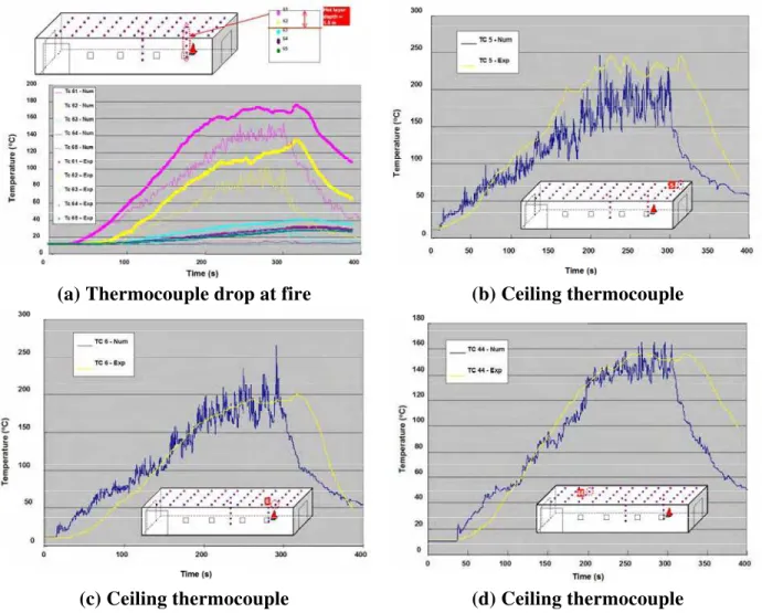
A 1.0 m x 1.75 m gasoline pool fire source was used in the demonstration test. A total heat release rate (HRR) of about 3.0 MW was predicted by the numerical simulation (Figure 2-2). Thermocouples (Type K) were distributed for temperature measurements (55 thermocouples were located at 150 mm below the ceiling of the tunnel facility). Two thermocouple trees (5 thermocouples each) were dropped from the ceiling of the tunnel. One was located above the fire to measure the gas/flame temperatures of the fire source. The second thermocouple tree was located at the middle of the tunnel.
Figure 2-1 Demonstration Test
Figure 2-3 shows the modelled domain, initial, and boundary conditions used in the numerical simulations for the demonstration test. The walls and the ceiling of the tunnel were modelled as concrete surfaces. The two end doors of the tunnel were closed during the test. The two side louvers at the East end of the tunnel, however, were partially opened, to provide an air supply for the fire. The opening of the two side louvers was 1.5 m wide by 4.9 m high for the North louver, and 2.75 m wide by 4.9 m high for the South louver.
Figure 2-3 Demonstration test: computational domain, initial and boundary conditions
Figure 2-4 shows sample comparisons of predicted and measured temperatures at the thermocouple drop close to the fire source (Figure 2-4a) and at different locations across the ceiling (Figure 2-4b, 2.4c, 2.4d). The discrepancies between the two set of data in Figure 2-4a may be attributed to the effect of radiation on the thermocouple readings which was not accounted for in the numerical model. Figure 2-4a indicates a hot layer depth of about 1.5 m from the ceiling. The effect of radiation reduces further from the fire source and thus Figure 2-4b, 2.4c, 2.4d shows good comparisons for the predicted and measured temperatures.
The results from the numerical simulations indicated that the airflow velocity within the tunnel was about 0.25 m/s and that the hot layer depth was about 1.5 m from the ceiling (Figure 2-4a). These predictions compare well with the measurements (during in-situ tests, smoke depth was measured to be about 1.2 m in the vicinity of fire and the airflow velocity was in the range of 0.15-0.20 m/s).
The results from these comparisons assisted in planning the instrument set-up and test procedures for the experimental program
2.2 Post Full-Scale Tests CFD Simulations
Three series, “A”, “B” and “C”, of CFD simulations were conducted, using FDS, to compare numerical predictions against test results. The following sections describe the results of the comparisons of the numerical predictions and the experimental data of Tasks 2, 4, and 7.
(a) Thermocouple drop at fire (b) Ceiling thermocouple
(c) Ceiling thermocouple (d) Ceiling thermocouple Figure 2-4 Numerical predictions versus experimental data – Demonstration test
2.2.1 Series A
Series A consisted of 11 simulations (Table 2-1) replicating the full-scale fire tests conducted in the tunnel facility under non-ventilated conditions. Two types of fire scenarios were simulated: pool fires (under and behind vehicles) and stationary vehicle fires (engine or passenger compartment), using the same dimensions as used in tests of Task 2 [4]. The fire sizes varied from approximately 100 KW to 3,400 kW with various growth rates (1 min to 12 min to reach their maximum heat release rates). The CFD simulations involved various fire locations (underneath a vehicle and behind a large vehicle) and various fuel types (gasoline, propane, wood crib and polyurethane foam). In general, the fire growth rate was adjusted to the growth of temperature measured in the tests (Table 2-1).
Table 2-1 provides a description of the simulations, the initial, and boundary conditions used in the numerical simulations. The two end doors of the tunnel were closed during the tests. The two side louvers at the east end of the tunnel, however, were partially opened, to provide air for the fire.
Table 2-1 CFD Simulations (Series A Tests - No ventilation) Airflow speed at Louvers (m/s) SCENARIO Simulation ID Fire Source Dimensions m x m Fuel Type HRR (KW) Tamb (oC) North South Ceiling Fan
Tun2UV1 0.6X0.6 gasoline 550~650 6 0.3 0.1 open
Tun2UV2 1.0X1.0 gasoline 1500~1700 1 0.2 0.4 open
Tun2UV3 1.0X2.0 gasoline 3000~3400 13 0.1 0.0 open
Fire under the vehicle
Tun2UV4 1.2X2.0 gasoline 1500~1700 10 open open open
Tun2BV5 0.3X0.3 gasoline 100~125 4 0.4 0.6 open
Tun2BV6 0.6X0.6 gasoline 550~650 7 1.5 open open
Tun2BV7 1.0X1.0 gasoline 1500~1700 9 0.6 0.6 open
Fire behind the vehicle
Tun2BV8 1.0X2.0 gasoline 3300~3400 11 1.0 1.0 open
Tun2EC9 Engine compartment gasoline ~2000 1 open open open
Tun2PC10 Passenger compartment wood crib 1100~1500 7 open open open
Stationary vehicle fire
Tun2PC11 Passenger compartment Polyurethane
The first 4 simulations; Tnu2UV1, Tnu2UV2, Tnu2UV3, and Tnu2UV4, replicated the tests conducted with a fire under a vehicle. Comparisons of temperature were made at several locations along the centerline of the tunnel ceiling and at different heights at the middle of the tunnel. Comparisons of smoke optical density (OD) were made on the vertical axis at mid-tunnel. The OD indicates the level of smoke obscuration. The higher the value of OD, the higher the smoke obscuration and the lower the visibility. The visibility, VIS, may be calculated from the OD as follows [Klote and Milke 2000]:
α
K
VIS =− (1)
where:
α = extinction coefficient, m-1 = 2.303 OD
K = proportionality constant, dimensionless (6 for illuminated signs, 2 for reflected signs and building components in reflected light)
VIS = visibility, m.
The NFPA 502 defines the smoke obscuration levels that should be considered to maintain a tenable environment. Smoke obscuration levels should be continously maintained below the point at which a sign illuminated at 80 lx (7.5 ft-candles) or equivalent brightness for internally luminated signs, is discrenible at 30 m (100 ft), and doors and walls are discrenible at 10 m (33 ft).
Figure 2-5 shows the temperature comparisons for the case of a 0.6 x 0.6 m gasoline pool fire under a vehicle. Figure 2-5b shows the predicted steady-state heat release rate (HRR) to be to be in the range of 600-800 kW, which is a little higher than the expected range of 550-650 kW. The HRR had a growth stage that continued for up to 150 s after ignition.
The comparisons of ceiling temperatures were, in general, favourable. The numerical predications were featured by fluctuations with rather large amplitudes especially at locations close to the fire (Figure 2-5d and e). The experimental results did not exhibit the same phenomenon \. This can be attributed to two reasons; the frequency of data collection was courser (1 Hz) than that for the numerical predictions (∼0.01 Hz). The plume shape was not perfectly replicated by the numerical procedure.
Figure 2-6 and Figure 2-7, show the same type of comparisons for the two cases, Tun2UV2 and Tun2UV3 for gasoline pool fires under a vehicle with sizes of 1.0 x 1.0 and 1.0 x 2.0 m, respectively. The predicted steady-state HRR of the two cases are shown in Figure 2-6b and Figure 2-7b. The predicted values were in the expected range of 1500-1700 kW for Tun2UV2 and 3000-3400 kW for Tun2UV3. The amplitudes of the numerical fluctuations were larger than those predicted for Tun2UV1. As the size of the pool fire increased the instability of the flames was more pronounced and hence the larger amplitudes for the fluctuations.
Figure 2-8 shows the comparisons of ceiling and vertical temperatures for Tun2UV4. In this case, the fuel was premixed propane supplied through 16 pipes. The fluctuations of the numerical predictions had smaller amplitudes indicating a more stable flame/plume. Figure 2-8c, d, e, and f show better comparisons between the numerical predictions and tests.
Figure 2-9, Figure 2-10, Figure 2-11, and Figure 2-12 show the comparison of results of the numerical predictions against the experimental results for the case of a fire behind a vehicle under minimal airflow conditions. In general, the comparisons were more favourable than those for the case of a fire under a vehicle. This can be attributed to the fact that the simulations of a fire under a vehicle represented a slightly under-ventilated fire condition. In general, FDS is more reliable for well-ventilated cases.
Figure 2-13, Figure 2-14, and Figure 2-15 show the comparison of results of the numerical predictions against the experimental results for passenger and engine compartment fires under minimal airflow conditions.
Figure 2-16 and Figure 2-17 show the comparison of results of the numerical predictions of smoke OD against the experimental results for the two cases of Tun2BV5 and Tun2BV8. The OD values were compared at three heights at the center of the tunnel; namely, 1.5 m, 2.5 m, and 5.35 m. Both figures indicate a smoke layer that travelled close to the ceiling. The fire scenario Tun2BV8 with a fire size of 1.0 m x 2.0 m produced a much higher OD at the height 5.35 m above tunnel floor than for the Tun2BV5 simulation. At the middle and lower heights, the OD values were quite small, especially for Tun2BV5. The comparisons were quite favourable for the OD values close to the tunnel ceiling (5.35 m height).
2.2.2 Series B
Series B consisted of 6 simulations (Table 2-2) replicating the full-scale fire tests conducted in the tunnel facility under ventilation conditions. Two types of fire scenarios were simulated: gasoline pool fires under and behind vehicles, using the same dimensions as used in tests conducted in Task 7 [5]. The fire sizes varied from approximately 550 KW to 3,400 kW. The ventilation was provided by operating the tunnel fans in exhaust mode drawing fresh air from the East end of the tunnel through the east door and south and north louvers. The fans were operated at three different capacities inducing airflows in the tunnel with three different speeds; 0.0, 1.5, and 3.0 m/s.
Table 2-2 describes the simulations, the initial, and boundary conditions used in the numerical simulations. The west end door of the tunnel was closed during the tests.
The first 4 simulations; Tun2UV21, Tun2UV22, Tun2UV23, and Tun2UV24, replicated the tests conducted for a fire under a vehicle. Figure 2-18 shows the temperature comparisons for the case Tun2UV21 of a 0.6 x 0.6 m gasoline pool fire under a vehicle with airflow speed of 0.0 m/s. Figure 2-18a shows the airflow speed at the east end of the tunnel close to the fire and at the middle section of the tunnel. Close to the fire, the airflow was predicted to be almost zero as measured in the test. At the middle of the tunnel, the airflow speed was predicted to be approximately 0.5 m/s as a result of convective flow produced by the fire. Figure 2-18b shows the predicted steady-state heat release rate (HRR) to be in the range of 600-800 kW (similar to the fire scenario Tun2UV1). The comparisons of ceiling (Figure 2-18d, e, f) and vertical (Figure 2-18c) temperatures were, in general, favourable.
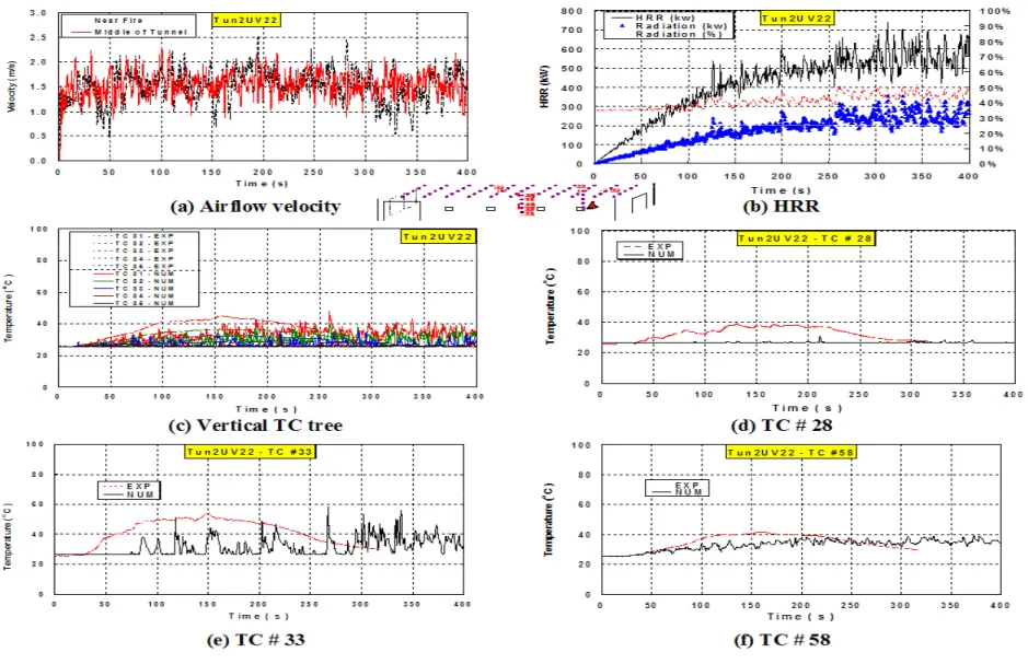
Figure 2-19 shows the same type of comparisons for Tun2UV22 for gasoline pool fires under a vehicle with a size of 0.6 m x 0.6 m and an airflow speed of 1.5 m/s. Figure 2-19a shows an average airflow speed of 1.5 m/s both close to the fire and at the middle of the tunnel. Close to the fire, the predicted airflow speed fluctuated with large amplitudes due to the turbulence occurring at the east tunnel entrance. The predicted steady-state HRR is shown in Figure 2-19b. The predicted values were in the range of 550-650 kW. The incoming airflow speed of 1.5 m/s tilted the fire plume limiting air-entrainment in the fire plume and thus reducing the HRR. This phenomenon was observed in the corresponding test. As a result, the predicted temperatures were, in general, lower than those of Tun2UV21. Moreover, both the radiation and turbulence at and close to the fire affected the quality of the numerical predictions at these locations. Away from the fire (Figure 2-19f), the quality of predications and hence the comparison was improved as the effect of both radiation and entrance turbulence was reduced.
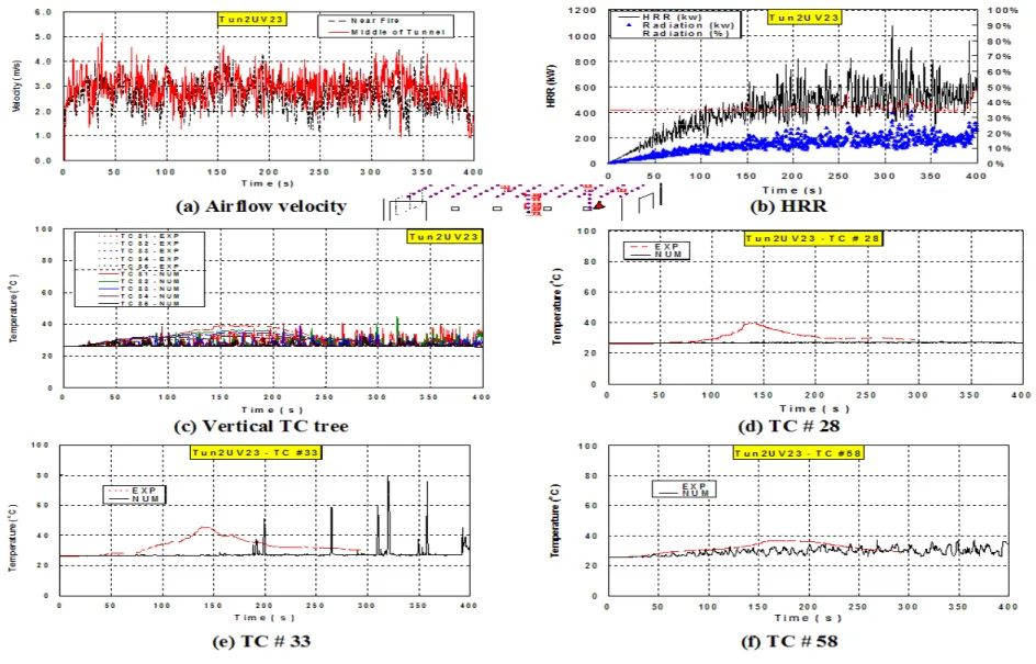
Figure 2-20 shows the comparisons of ceiling and vertical temperatures for Tun2UV23. In this case, the airflow speed was 3.0 m/s (Figure 2-20a). In general, lower temperatures than those of Tun2UV21 and Tun2UV22 were predicted due to the higher airflow speed. The numerical simulations showed almost ambient temperature close to the fire. However, at the middle of the tunnel and away from the fire, the numerical predictions were improved and good comparisons were observed.
Figure 2-21 shows the comparison of results of the numerical predictions against the experimental results for Tun2UV24. Figure 2-21a shows the predicted airflow speeds at the east end entrance and at the middle of the tunnel. At the east entrance, the average airflow speed was predicted to be 1.5 m/s. At the middle of the tunnel, however, the average airflow speed was about 2.5 m/s. The increase of airflow speed can be attributed to the of the large fire. Discrepancies between numerical predictions and test results were observed close to the fire. Away from the fire (Figure 2-21f), the comparison was more favourable.
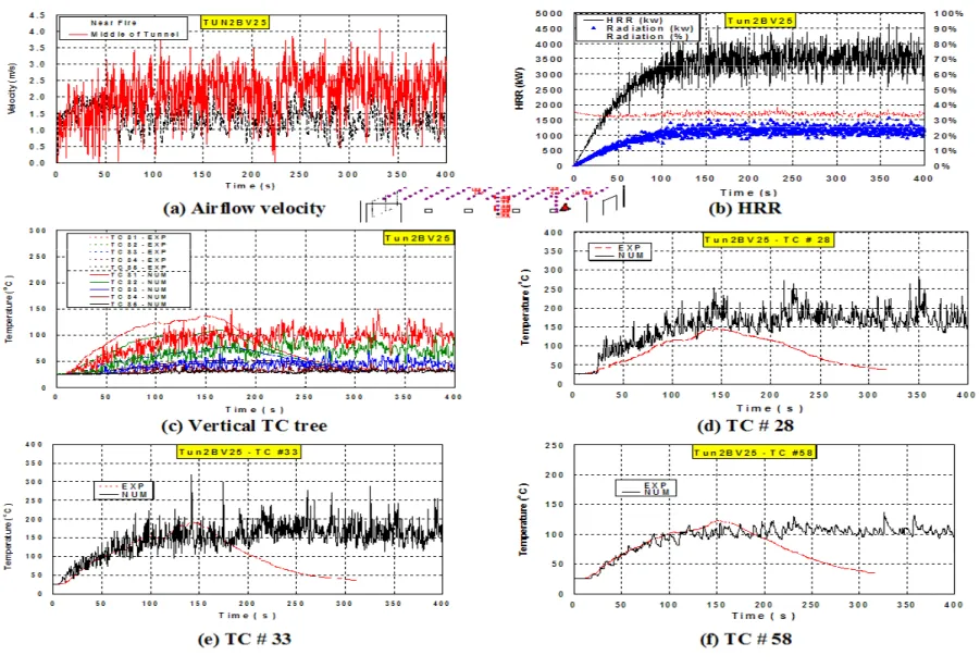
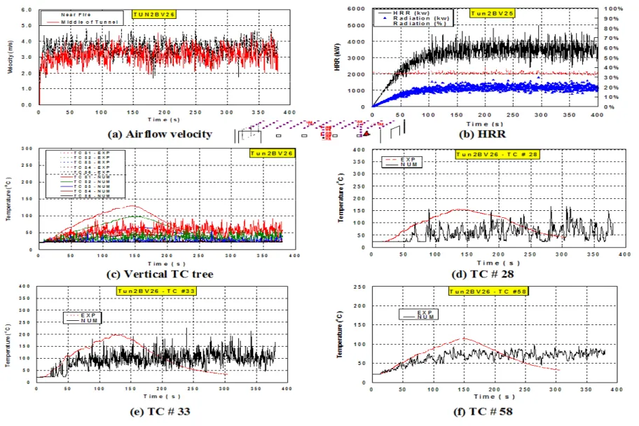
Figure 2-22 and Figure 2-23 show the comparison of results of the numerical predictions against the experimental results for the scenario with a fire behind a vehicle, Tun2UV25 and Tun2UV26. In general, the comparisons were more favourable than those for the case of a fire under a vehicle, especially for Tun2UV25 with an airflow speed of 1.5 m/s. When the airflow speed was doubled, Tun2UV26, the strong incoming airflow tilted the fire plume and reduced the radiation to the tunnel ceiling. As a result, lower temperatures than those for Tun2UV25 were predicted.
Figure 2-24 and Figure 2-25 show the comparison of results of the numerical predictions of smoke OD against the experimental results for the two cases of Tun2UV22 and Tun2BV25. The numerical predictions of Tun2UV22 (Figure 2-24) indicated that the smoke spread close to the tunnel floor as a result of a strong deflection of the fire plume. However, for Tun2BV25 the ceiling jet and hence the upper smoke layer phenomena were observed indicating lower plume deflection.
Table 2-2 CFD Simulations (Series B Tests - With ventilation) Airflow speed at Louvers (m/s) SCENARIO Simulation ID Fire Source Dimensions (m) x (m) Fuel Type HRR (KW) Tamb (oC) Airflo w Speed (m/s) North South Ceiling Fan m3/s
Tun2UV21 0.6X0.6 gasoline 550~650 22.3 0.0 open open open
Tun2UV22 0.6X0.6 gasoline 550~650 25.6 1.5 open open 62
Tun2UV23 0.6X0.6 gasoline 550~650 25.8 3.0 open open 124
Fire under the vehicle
Tun2UV24 1.0X2.0 gasoline 3000~3400 24.5 1.5 open open 62
Tun2BV25 1.0X2.0 gasoline 3300~3400 25.5 1.5 open open 62
Fire behind the vehicle
2.2.3 Series C
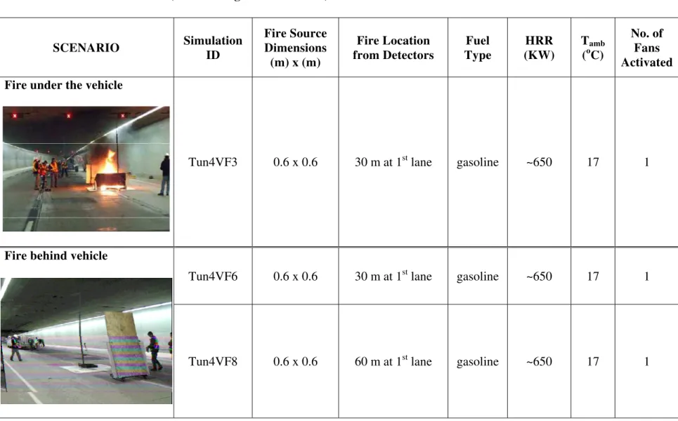
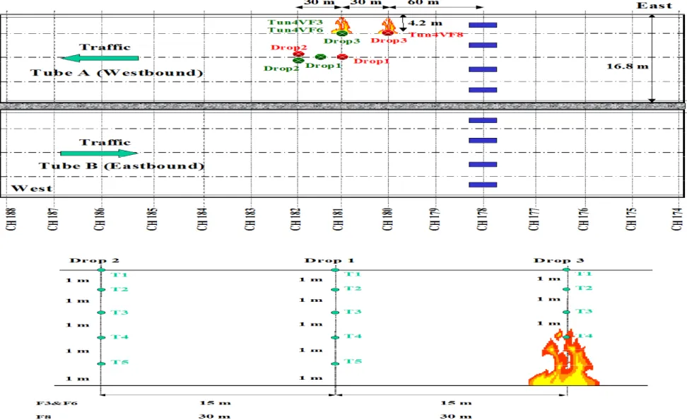
Series C consisted of 3 simulations (Table 2-3) replicating the field tests that were conducted in Tube A of the Carré-Viger Tunnel in Montreal (Figure 2-26). Two types of fire scenarios were simulated: gasoline pool fires under and behind vehicles, using the same dimensions as used in the tests conducted for Task 4 [6]. The fire size was approximately 650 KW for the three simulations. The tunnel had a longitudinal ventilation system that was equipped with eight ceiling jet fans (4 fans in each tube). The capacity of each jet fan was 50,000 and 30,000 m3/s in the supply and exhaust modes, respectively. Each jet fan can operate on its own or in combination with the other fans. The ventilation flows can be adjusted as needed. For all the CFD simulations, only one jet fan was activated.
Both predicted temperature and smoke OD were compared against the field data. Temperatures were monitored at three different vertical locations (Drops) corresponding to the thermocouple trees used in the tests (Figure 2-26). Drop 3, with four vertical thermocouples spaced at 1.0 m intervals starting 2 m above the tunnel floor. For Tun4VF3 and Tun4VF3, Drops 1 and 2 were placed at the middle of the tunnel 15 m and 30 m, respectively, from the fire source. For Tun4VF8, Drops 1 and 2 were placed at 30 m and 60 m, respectively, from the fire source. There were five thermocouples at each of the two drops spaced at 1.0 m intervals starting 1 m above the tunnel floor. Smoke OD values were monitored at two heights, 4.75 m and 2.45 m above the tunnel floor, at both Drop 1 and 2. The first smoke meter in the thermocouple tree was located near the ceiling and the other smoke meter was 2.3 m from the tunnel ceiling.
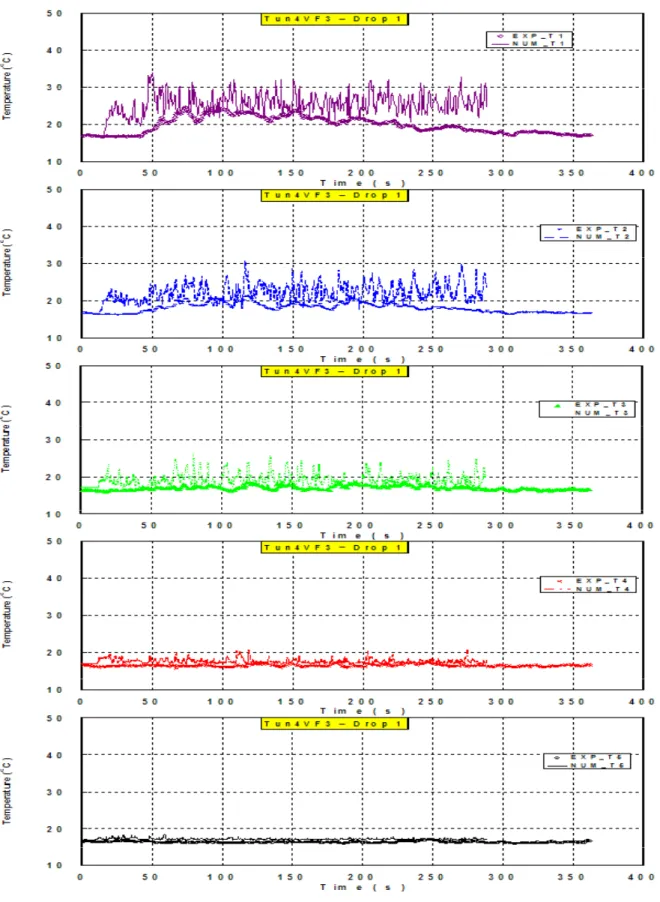
Figure 2-27, Figure 2-28, and Figure 2-29 show the temperature comparison at Drops 1, 2, and 3, respectively for Tun4VF3 (0.6 m x 0.6 m gasoline pool fires under vehicle). Away from the fire source at Drops 1 and 2, the comparisons of temperatures at various heights were reasonable (Figure 2-27, Figure 2-28). The numerical predictions exhibited fluctuating behaviour. However, the average of the predictions compared well with the test results.
At the fire source (Figure 2-29), discrepancies between numerical and experimental data were observed. The highest temperature was recorded close to the ceiling (T4) for the experimental data and at 2 m from the ground for numerical predictions (T1). This can be attributed to different plume tilts (the plume was tilted more in the numerical simulations). However, the maximum temperatures for both experimental and numerical were the same (30oC) at the T1 location for the numerical simulation and T4 for the experiments.
Figure 2-30 shows the smoke OD comparisons at two heights at Drops 1 and 2. Both numerical predictions and experimental data indicated that a smoke layer was formed near the ceiling as indicated by the higher smoke meter (SM1) at the two drops (Figure 2-30a and c). Lower OD values were recorded by the lower smoke meters (SM2).
Figure 2-31, Figure 2-32, Figure 2-33, and Figure 2-34 show the temperature and smoke comparisons at Drops 1, 2, and 3, respectively for Tun4VF6 (0.6 m x 0.6 m gasoline pool fires behind a vehicle). Similar to Tun4VF3, temperature and OD values were comparable at the two drops 1 and 2. The same difference in the temperature was observed
at Drop 3. In this case, the maximum temperature in the tests and simulations was about 80oC.
Figure 2-35, Figure 2-36, Figure 2-37, and Figure 2-38 show the temperature and smoke comparisons at Drops 1, 2, and 3, respectively for Tun4VF8 (0.6 m x 0.6 m gasoline pool fires behind a vehicle). Similar to Tun4VF3 and Tun4VF8, the experimental and simulation temperatures were reasonably comparable at drops 1 and 2. However, large differences in temperature were observed at Drop 3. In general, the numerical predictions were much lower than the experimental data. In this case, the fire source was placed closer to the jet fan. The predicted airflow speeds were larger than those measured in the field, which led to a faster dilution of the smoke from the fire. This was confirmed by the predicted smoke OD values (Figure 2-38).
2.3 Conclusions
Twenty CFD simulations were conducted to replicate laboratory and field full-scale experiments. The simulations covered different fire sizes, location, ventilation scenarios, and fuel type. Comparisons of temperature and smoke OD were made at different locations corresponding to lab and field measurements points.
In general, favourable comparisons between the numerical predictions and experimental data were observed. Discrepancies were observed in some comparisons. Both radiation and turbulence at and close to the fire source had a significant effect on the numerical predictions at these locations. For large fire sizes and highly turbulent situations, these effects were more pronounced. Away from the fire, the predications and hence the comparison with the experimental results were improved as the effect of both radiation and turbulence was reduced.
The numerical predications fluctuated with large amplitudes especially at locations closer to the fire. The experimental results did not exhibit the same fluctuations. This can be attributed to two reasons; the frequency of data collection was course and the plume shape was not properly replicated in the numerical simulation. As the size of the pool fire increased, the instability of the flames was more pronounced and hence larger fluctuations were observed.
In some cases where the fire plume was deflected differently in the simulation than was observed in the corresponding full-scale test, the vertical temperature profile close to the fire was altered and the maximum plume temperature was shifted up or down depending on the angle of deflection of the plume.
In general, the comparisons were more favourable for the scenario with the fire behind a vehicle than those for the case with a fire under a vehicle. This can be attributed to the fact that the fire under a vehicle represented partially under-ventilated fire conditions. In general, FDS is more suited for well-ventilated cases.
Table 2-3 CFD Simulations (Series C Viger Tunnel Tests) SCENARIO Simulation ID Fire Source Dimensions (m) x (m) Fire Location from Detectors Fuel Type HRR (KW) Tamb (oC) No. of Fans Activated Fire under the vehicle
Tun4VF3 0.6 x 0.6 30 m at 1st lane gasoline ~650 17 1
Tun4VF6 0.6 x 0.6 30 m at 1st lane gasoline ~650 17 1
Fire behind vehicle
3
INVESTIGATION OF THE IMPACT OF DIFFERENT
PARAMETERS ON FIRE BEHAVIOR AND DETECTION SYSTEM
PERFORMANCE
This section presents the results of the CFD simulations conducted to investigate the impact of various parameters on fire behaviour and detection system performance. The investigated parameters included: fire scenarios, ventilation mode, and tunnel length.
3.1 Ventilation Systems
In general, there are three main types of ventilation systems in roadway tunnels: longitudinal, full-transverse, and semi-transverse ventilation systems (Figure 3-1) [9]. The longitudinal ventilation type (Figure 3-1a) creates a longitudinal flow along the roadway tunnel by introducing or removing the air from the tunnel at a limited number of points. The ventilation air is provided either by injection, by jet fans, or by a combination of injection or extraction at intermediate points in the tunnel. The longitudinal form of ventilation is the most effective method of smoke control in a highway tunnel with unidirectional traffic.
Full-transverse ventilation systems (Figure 3-1b) are used in long tunnels and in tunnels with heavy traffic volume. This ventilation system comprises both a supply and an exhaust duct to achieve uniform distribution of supply air and uniform collection of vitiated air throughout the tunnel length. This configuration produces a uniform pressure along the roadway with no longitudinal airflow being generated except that created by the traffic piston effect.
Semi-transverse ventilation systems (Figure 3-1c and d) can either consist of a supply system or an exhaust system. This type of ventilation incorporates the distribution of (supply system) or collection of (exhaust) air uniformly throughout the length of a road tunnel. Semi-transverse ventilation is normally used in tunnels up to about 7000 ft (2134 m); beyond that length the tunnel air speed near the portals becomes excessive.
3.2 CFD Simulations – Series D
To investigate the effect of ventilation types on the fire dynamics and consequently on the detection system performance, 7 CFD simulations were conducted. The simulations were conducted for a road tunnel similar to the laboratory tunnel test facility but with different ventilation systems.
Table 3-1 summarizes the simulations. Two pool fire sizes were used: 1.0 m x 1.0 m and 1.0 x 2.0 m. An ambient temperature of 20oC was assumed. Four types of ventilation systems were used (Figure 3-1): longitudinal (LT), full-transverse (FT), semi-transverse (supply – ST1 & ST2), and semi-transverse (exhaust – ST3 & ST4).
For all simulations except for Tun2LT1, the two tunnel ends (portals) were modelled as “OPEN”, i.e. atmospheric pressure. For simulations Tun2ST1 and Tun2ST2 (Figure 3-1c) fresh air was supplied from the tunnel floor. The volumetric flow rate of supplying air was 11.47 m3/s. This value was based on current recommended ventilation fire safety guideline of 100 cubic feet per minute per lane-foot airflow rate [10]. For Tun2ST3 and Tun2ST4 (Figure 3-1d) smoke and fire products were exhausted through the tunnel ceiling at a rate of 11.47 m3/s. For Tun2FT1 and Tun2FT2 (Figure 3-1b) fresh air was supplied from the tunnel floor and smoke and fire products were exhausted through the tunnel ceiling at equal rates of 11.47 m3/s. An inlet airflow speed of 3 m/s at the west portal (Figure 3-1a) was assumed for Tun2LT1 to represent a prevailing wind condition at that end of the tunnel.
Figure 3-2 shows the plots of the airflow speeds along a vertical axis at the middle of the tunnel for the 7 CFD simulations. Among all the simulations, Tun2LT1 with longitudinal ventilation scheme produced a quasi-steady state velocity profile at the middle of the tunnel. Moreover, the vertical velocity profile had a uniform velocity with height up to near the ceiling (Figure 3-4). The airflow speed achieved its steady state in less than 20 s. The other ventilation systems produced velocity profiles with mainly a vertical velocity component with a longitudinal velocity component produced near the ceiling (Figure 3-4). Moreover for all other ventilation systems, the airflow speed attained steady-state at approximately 100 s. The time at which the velocity field reaches steady-state condition will affect the rate of temperature rise in the tunnel and hence the performance of the detection systems.
Figure 3-3 shows the plots of the temperature on the vertical axis at the middle of the tunnel for the 7 CFD simulations. In Tun2LT1, the temperature was maintained at ambient conditions. The rate of ceiling temperature rise up to the steady-state conditions at the middle of the tunnel for Tun2FT1, Tun2FT2, Tun2ST1, Tun2ST2, Tun2ST3 and Tun2ST4 was 0.13, 0.40, 0.30, 0.67, 0.10, 0.40oC/s, respectively. As such, Tun2ST2 resulted in the fastest rate of rise of ceiling temperature. On the other hand, Tun2ST3 resulted in the slowest rate of rise of ceiling temperature.
Figure 3-5 and Figure 3-6 show the average temperature along the tunnel ceiling and along a vertical axis at the middle of the tunnel, respectively, for the seven CFD simulations. For the same fire size, the semi-transverse supply ventilation system (Tun2ST1 and Tun2ST2) resulted in the highest ceiling temperature. Both the full- and semi-transverse exhaust ventilation systems produced a similar average ceiling temperature profile. Tun2LT1 resulted in the lowest average ceiling temperature.
Figure 3-7 shows the average soot volume fraction in ppm along the tunnel ceiling for the seven CFD simulations. For the same fire size, the semi-transverse supply ventilation system (Tun2ST1 and Tun2ST2) resulted in the highest ceiling soot concentration. Both the full- and semi-transverse exhaust ventilation systems produced similar average ceiling soot profiles. Tun2LT1 resulted in the lowest average ceiling soot concentration.
Table 3-1 Effect of Ventilation Type (Series D - Fire behind a vehicle)
Ventilation Type Simulation ID Fire Source Dimensions (m) x (m) Fuel Type HRR (KW) Airflow Injected (exhausted) (m3/s) Tamb (oC) Wind at both portals (m/s) Tun2ST1 1.0X1.0 Gasoline 1500~1700 11.47 (0) 20 open (open) Semi transverse Tun2ST2 1.0X2.0 Gasoline 3300~3400 11.47 (0) 20 open (open) Tun2ST3 1.0X1.0 Gasoline 1500~1700 (0) 11.47 20 open (open) Semi transverse Tun2ST4 1.0X2.0 Gasoline 3300~3400 (0) 11.47 20 open (open) Tun2FT1 1.0X1.0 Gasoline 1500~1700 11.47 (11.47) 20 open (open) Fully transverse Tun2FT2 1.0X2.0 Gasoline 3300~3400 11.47 (11.47) 20 open (open) Longitudinal Tun2LT1 1.0X1.0 Gasoline 1500~1700 (0) (0) 20 open (3)
3.3 CFD Simulations – Series E
To investigate the effect of ventilation type and tunnel length on the fire dynamics and consequently on the performance of detection systems, three CFD simulations were conducted. The simulations were conducted for a road tunnel 500 m long, 12.0 m wide (three lanes), and 5.5 m high.
Table 3-2 summarizes the different conducted simulations. A pool fire size of 1.0 m x 1.0 m placed behind a vehicle was used in the three simulations. An ambient temperature of 20oC was assumed. Three ventilation conditions were simulated (Figure 3-8); longitudinal systems, full-transverse, and no ventilation.
For simulations Tun2DFT1 and Tun2DNV1, the two tunnel portals were modelled as “OPEN”, i.e. atmospheric pressure. For simulations Tun2DFT1 (Figure 3-8b), fresh air was supplied from the tunnel floor and smoke and fire products were exhausted through the tunnel ceiling at equal rates of 230 m3/s. An inlet airflow speed of 3 m/s at the east portal (Figure 3-8a) was assumed for Tun2DLT1 to represent a prevailing wind condition at that end of the tunnel.
Figure 3-9 shows the longitudinal airflow speeds along a vertical axis at the middle section of the tunnel. For Tun2DFT1 and Tun2DNV1, the longitudinal velocity components were predicted to be almost zero. For Tun2DLT1, an average longitudinal velocity component of about 6.0 m/s was predicted at mid-tunnel. This high value can be attributed to the effects of the fire and the presence of a large obstruction downstream the fire source.
Figure 3-10 shows the average temperature profile along the middle of the tunnel ceiling near the fire source. At the fire source, Tun2DLT1 produced the lowest ceiling temperature because the airflow around the fire pushed smoke and hot gases downstream of the fire. Therefore, higher ceiling temperatures downstream of the fire were predicted. Tun2DNV1 resulted in the highest ceiling temperature at and around the fire source. This ventilation scheme produced a symmetrical temperature field around the fire source. Tun2DFT1 resulted in the lowest ceiling temperature at a distance of 35 m downstream of the fire source.
Figure 3-11 shows the average vertical temperature profile at mid-tunnel downstream of the fire. Tun2DLT1 resulted in the highest vertical temperature profile as the flame was tilted the most in this scenario. Tun2DNV1 produced the highest temperature close to the ceiling indicating a strong ceiling jet of hot gases and smoke.
Figure 3-12 shows the average soot volume fraction values along the middle of the tunnel ceiling around the fire source. Tun2DNV1 resulted in the highest soot values. While, Tun2DLT1 produced the lowest soot values at the fire and the tunnel was filled with soot downstream of the fire.
Figure 3-13, Figure 3-14, and Figure 3-15 show 3D renders of smoke and temperature for Tun2DFT1, Tun2DNV1, and Tun2DLT1, respectively. Figure 3-13, for Tun2DFT1, shows that the fully transverse ventilation system resulted in the highest temperatures and smoke densities at the tunnel ceiling around the fire source.
For Tun2DNV1 (Figure 3-14), smoke and hot gases spread symmetrically downstream and upstream of the fire to large distances. The ceiling jet entrained fresh air as it travelled along the tunnel eventually losing its buoyancy and descended to lower heights.
Figure 3-15, for Tun2DLT1, shows the longitudinal ventilation pushed hot gases and smoke downstream of the fire. The results indicate extensive tilting of the fire plume towards the downstream side of the fire. As a result, the smoke filled the height of the tunnel downstream of the fire.
Table 3-2 Effect of Ventilation Type (Series E - Fire behind a vehicle)
Ventilation Type Simulation ID Fire Source Dimensions (m) x (m) Fuel Type HRR (KW) Airflow Injected (exhausted) (m3/s) Tamb (oC) Wind at both portals (m/s) Longitudinal
Tun2DLT1 1.0X1.0 Gasoline 1500~1700 0 (0) 20 Open
(3)
No ventilation
Tun2DNV1 1.0X1.0 Gasoline 1500~1700 0 (0) 20 Open
(open)
Fully transverse
Tun2DFT1 1.0X1.0 Gasoline 1500~1700 230 (230) 20 Open (open)
3.4 Effect of Tunnel Length
Figure 3-16, Figure 3-17, Figure 3-18, and Figure 3-19 compare the velocity, ceiling and vertical temperature, and soot volume fraction profiles, respectively, for two similar tunnels with different lengths (37.5 m and 500 m).
Figure 3-16 shows the average longitudinal velocity component profile at the mid-tunnel section for the two mid-tunnel lengths and for three ventilation cases: full-transverse, longitudinal, and no ventilation. Both the full-transverse and no ventilation cases produced very similar velocity profiles for the two lengths. For the longitudinal ventilation system, similar velocity profiles were produced. However, higher velocities were produced in the case of the 500 m tunnel length.
Figure 3-17 and Figure 3-19 show the comparisons of the ceiling temperatures and soot volume fractions for the two tunnel lengths. Both temperature and soot profiles were very similar for the two lengths. As such, the length of the tunnel had no significant effect on the ceiling temperature and smoke density.
Figure 3-18 shows the average vertical temperature profile at the mid-tunnel section for the two length tunnels and the three ventilation cases. Both the full-transverse and no ventilation cases produced similar profiles for the two lengths. For the longitudinal ventilation system, similar profiles were produced. However, higher velocities were produced in the case of the 500 m tunnel length.
3.5 Conclusions
Four types of ventilation systems and two tunnel lengths were investigated. The ventilation systems included: longitudinal, full-transverse, semi-transverse (supply), and semi-transverse (exhaust). The two tunnel lengths were 37.5 m and 500 m. The 37.5 length is the same length as laboratory tunnel facility.
Among the ventilation schemes, the semi-transverse supply ventilation system resulted in the highest ceiling temperature and soot volume fraction. Both the full- and semi-transverse exhaust ventilation systems produced similar average ceiling temperature and soot profiles. The longitudinal ventilation system resulted in the lowest average ceiling temperature. The semi-transverse supply ventilation system resulted in the fastest rate of rise of ceiling temperature and the semi-transverse exhaust ventilation system resulted in the slowest rate of rise of ceiling temperature.
The ceiling temperature and soot volume fraction profiles for the two tunnel lengths were very similar implying that the length of the tunnel has limited effect on the ceiling temperature and smoke density.
In certain cases, the ventilation system or the prevailing wind could result in a strong longitudinal airflow in the tunnel causing a significant tilting of the fire plume. This could, in turn, result in the shift of the hot spot and sometimes, depending on the strength of the airflow, could slow or even prevent the formation of a hot layer. In these cases, the performance of detection systems that rely on absolute temperature or rate of temperature rise to detect fire incident may be compromised. Moreover, the strong longitudinal airflow may disrupt the structure of the fire plume altering its regular shape. Consequently, it becomes quite challenging for detection systems that depend on visualizing the flame to detect the fire incident.
The existence of stopped traffic in the tunnel could influence the flow field in the tunnel. It may lead to faster flow in some areas resulting in lower temperatures or to pockets of stagnant air resulting in higher temperatures. Moreover, it may obstruct the viewing zone of detection systems causing a delay in detecting the fire. Although traffic patterns were not investigated in the current study, the existence of an obstruction in the tunnel can affect the fire dynamics.
In general, the data predicted from the CFD simulations can be efficiently related to the performance of spot heat detectors, linear heat detection systems, and smoke aspiration detection systems. However, more effort is required to relate CFD data to the video imaging detection (VID) and flame detection systems. CFD can provide temporal and spatial information on the expected shape of the plume, heat flux, wall temperature, which may be useful in linking the simulation results to the performance of optical-based detection system.
4 REFERENCES
1. Zalosh, R and Chantranuwat, P., “International Road Tunnel Fire Detection Research Project, Phase 1: Review of Prior Test Programs and Tunnel Fires,” The Fire Protection Research Foundation, November 2003.
2. K.B. McGrattan, “Fire Dynamics Simulator (Version 4) – Technical Reference Guide”, NIST Special Publication 1018, National Institute of Standards and Technology, Gaithersburg, MD, 2005.
3. Z. G. Liu, G. P. Crampton, A. H. Kashef, G. D. Lougheed, E. Gibbs, J. Z. Su and N. Benichou, “ International Road Tunnel Fire Detection Research Project – Phase II: Task 1, Fire Detectors, Fire Scenarios and Test Protocols,” NRCC Client Report (B-4179.1), July 2006.
4. Z. G. Liu, G. P. Crampton, A. H. Kashef, G. D. Lougheed, E. Gibbs, and S. Muradori “ International Road Tunnel Fire Detection Research Project – Phase II: Task 2, Full-Scale Fire Tests in A Laboratory Tunnel” NRCC Client Report (B-4179.2), November 2007.
5. Z. G. Liu, G. P. Crampton, A. H. Kashef, G. D. Lougheed, E. Gibbs, and S. Muradori “ International Road Tunnel Fire Detection Research Project – Phase II: Task 7: Full-Scale Ventilated Fire Tests in a Laboratory Tunnel for Study of Fire Detection Technologies” NRCC Client Report (B-4179.2), February 2008.
6. Z. G. Liu, G. P. Crampton, A. H. Kashef, G. D. Lougheed, E. Gibbs, and S. Muradori “ International Road Tunnel Fire Detection Research Project – Phase II: Task 4: Field Fire Tests on Performance of Fire Detection Systems in an Operating Road Tunnel At Montreal City” NRCC Client Report (B-4179.2), February 2008.
7. NFPA 502 2001. Standard for Road Tunnels, Bridges, and Other Limited Access Highways. NFPA, 1 Batterymarch Park, PO Box 9101, Quincy, MA 02269-9101, USA.
8. Klote, J., and Milke, J. 2000. Principles of Smoke management. ASHRAE, Inc., 1791 Tullie Circle NE, Atlanta, GA 30329.
9. Kashef, A., Bénichou, N., Lougheed, G.D., Numerical Modelling of Movement and Behaviour of Smoke Produced from Fires in the Ville-Marie and L.-H.-La Fontaine Tunnels - Literature Review, pp. 74, September 01, 2003.
10. Massachusetts Highway Department and Bechtel/Parsons Brinckerhoff, “Memorial Tunnel Fire Test Ventilation Program – A comprehensive Test Report”, Massachusetts Highway Department, 1995.