Analysis of Atmospheric Delays and Asymmetric
Positioning Errors in the Global Positioning
A
System
yby
JUN
10
201
Kathryn Materna
LIBRARIE
Submitted to the Department of Earth, Atmospheric, and Planetary
Science
in partial fulfillment of the requirements for the degree of
Bachelor of Science in Earth, Atmospheric, and Planetary Science
at the
MASSACHUSETTS INSTITUTE OF TECHNOLOGY
June 2014
@
Massachusetts Institute of Technology 2014. All rights reserved.
Signature redacted
A uth or ...
...
Department of Earth, Atmospheric, and Planetary Science
May 16, 2014
Certified by...
Signature redacted...
Thomas A. Herring
Professor
Thesis Supervisor
Accepted
by..
Signature redacted...
Richard P. Binzel
Chairman, Committee on Undergraduate Program
Analysis of Atmospheric Delays and Asymmetric Positioning
Errors in the Global Positioning System
by
Kathryn Materna
Submitted to the Department of Earth, Atmospheric, and Planetary Science on May 16, 2014, in partial fulfillment of the
requirements for the degree of
Bachelor of Science in Earth, Atmospheric, and Planetary Science
Abstract
Errors in modeling atmospheric delays are one of the limiting factors in the accuracy of
GPS position determination. In regions with uneven topography, atmospheric delay
phenomena can be especially complicated. Current delay models used in analyzing
GPS data from the Plate Boundary Observatory (PBO) are successful in achieving
millimeter-level accuracy at most locations; however, at a subset of stations, the time series for position estimates contain an unusually large number of outliers. In many cases these outliers are oriented in the same direction. The stations which exhibit asymmetric outliers occur in various places across the PBO network, but they are especially numerous in California's Mammoth Lakes region, which served as a case study for this project. The phenomenon of skewed residuals was analyzed
by removing secular trends and variations with periods longer than 75 days from
the signal using a median filter. The skewness of the station position residuals was subsequently calculated in the north, east and up directions. In the cases examined, typical position outliers are 5-15 mm. In extreme cases, skewed position residuals, not related to snow on antennas, can be as large as 20 mm. I examined the causes of the skewness through site-by-site comparisons with topographic data and various forms of weather data such as numerical weather models, radiosondes, and satellite images. Analysis suggests that the direction of the skewness is generally parallel to the local topographic gradient at a scale of several kilometers. Comparison with weather data suggests that outlier data points in the Mammoth Lakes region occur when lee waves are likely to form downstream of the Sierra Nevada Mountains. The results imply that coupling between the atmosphere and local topography, e.g. lee waves, is responsible for the phenomenon of skewed residuals.
Thesis Supervisor: Thomas A. Herring Title: Professor
Acknowledgments
I am extremeley grateful to Professor Tom Herring for his guidance in forming this project and for his expertise. I am grateful for the technical help and insightful suggestions he provided. I would also like to thank the rest of Professor Herring's group, especially Mike Floyd for his help at the start of the project. I am grateful to Professor Dan Cziczo for making himself available on multiple occasions to answer my questions about atmospheric science and suggest possible directions.
I'd also like to thank my family and friends for their support. I especially
Contents
1 Introduction 10
1.1 B ackground . . . . 12
1.1.1 GPS Data Processing . . . . 12
1.1.2 Atmospheric Lee Waves . . . . 15
2 Methods 19 2.1 Sources of D ata . . . . 19
2.2 Determining Skewness . . . . 20
2.3 Determining Spatial Patterns of Skewness . . . . 21
2.4 Determining Temporal Patterns of Skewness . . . . 22
2.5 Examining Phase Residuals . . . . 23
3 General Results: Skewness in the PBO Network 25 3.1 General Characteristics of Skewness in the PBO Network . . . . 25
3.2 The Relationship Between Skewness and Local Topography . . . . 29
4 Case Study: Outliers in the Sierra Nevada 33 4.1 NW M Results . . . . 34
4.2 Radiosonde Results . . . . 36
4.3 M O D IS Results . . . . 38
4.4 Phase Residual Results . . . . 39
5 Discussion and Conclusion 42 5.1 Summary and Interpretation of Results . . . . 42
5.2 Possible Mechanisms for Position Errors . . . . 44
5.3 Future Directions . . . . 47 5.4 Conclusion . . . . 48
List of Figures
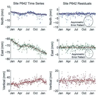
1-1 GPS time series for Site P642, a station in the Mammoth Lakes region
of the Sierra Nevadas. The second set of graphs shows the same time series with the long-term trend removed so that the position errors are more apparent. Note the numerous position errors of -5 to -10 millime-ters in the North and East directions, in contrast to the relatively few errors in the positive portion of each graph. . . . . 11
3-1 The PBO Network color-coded by station skewness. Red sites have the highest values of skewness. . . . . 27 3-2 A map of the Western United States highlighting the dense region
of highly-skewed stations in the eastern part of California. Another striking feature is the lack of skewed stations in the Central Valley. . 28 3-3 Skewness vectors on a topographic map of Mammoth Lakes, California.
Arrows represent the direction and magnitude of the skewness vector. 29
3-4 The alignment between skewness vector and locally high topography at six GPS stations: A) P142, Eastern Nevada; B) P388, Oregon; C)
P525, Central California coast; D) P612, Los Angeles, California; E) P635, Mammoth Lakes, California; F) TJRN, Santa Barbara,
Califor-nia. Note that the angle between the skewness vector and the topo-graphic gradient is small in each case. . . . . 31
3-5 The relationship between topographic gradients and the skewness vec-tor at various length scales. The histograms show distributions in the angle 0, the angle between the skewness vector and the local topo-graphic gradient vector. The gradients at a scale of 3 to 5 kilometers are most closely aligned with the skewness vectors. . . . . 32
4-1 The NAM output on November 30, 2012 for the region above Mammoth Lakes, CA. The wind vectors shown are at the 300 millibar surface, which is at approximately 9 kilometers above sea level. The average velocity is 21 m /s. . . . . 34 4-2 Wind roses for the NAM-derived wind velocity estimates at 300
mil-libar surface above station P643. Plot A shows the wind velocities on days with non-outliers in the GPS data at station P643, and Plot B shows the wind velocities on days with outliers in the GPS data at station P 643. . . . . 35
4-3 Plot A: Radiosonde-derived wind velodity as a function of elevation at Oakland during 2012. The GPS data are from station P642; red indicates that station P642 recorded an erroneous measurement within the highest 4% of its data on that day. Plot B: average wind velocity on outlier days and non-outlier days over the year. The error bars are the standard error of the mean velocity. . . . . 36
4-4 The average Brunt-Viisdld frequency as measured from Oakland Air-port during the year 2012. The red curve represents the average Brunt-Vdisdld frequency on days when station P642 recorded erroneous mea-surements within the highest 4% of its data. . . . . 37
4-5 Lee waves in the Sierra Nevada on March 13, 2012, as observed by the
4-6 Sky maps of phase residuals at station P643. March 28, 2012 showed
both elevated RMS scatter in the phase residuals and a large outlier in the GPS data. The surrounding days have lower phase residuals and normal position measurements. . . . . 40 4-7 At station P642, a large outlier measurement (6.81 mm) was made on
March 27, 2012. The phase residuals did not show higher scatter on that day. The phase residuals did show elevated RMS scatter on March
List of Tables
3.1 Skewness Values at Selected GPS Stations . . . . 26 3.2 Skewness in the PBO Network of GPS Stations . . . . 26
Chapter 1
Introduction
Over the past several decades, the Global Positioning System (GPS) has become the most common method among scientists for measuring position around the globe. Currently, daily-averaged GPS measurements can achieve accuracies at the millimeter level, and even at the sub-millimeter level in optimal cases. The high sensitivity of
GPS allows for the detection of small-amplitude phenomena such as tectonic
defor-mation, solid earth tides, and post-seismic offsets after earthquakes. Consequently,
GPS has become an important tool for many types of geophysical research.
Many of the GPS stations in the United States are part of the Plate Boundary Observatory (PBO) network. The Plate Boundary Observatory manages about 1,100 continuously-operating GPS stations throughout the United States for geophysical monitoring and research. Each station produces position estimates in the North, East, and Up directions each day, with typical position errors at these stations between 1 and 10 millimeters. For scientists who use the data to study the tectonics of North America, it is important for these measurements to be as accurate as possible.
It is observed that several GPS stations in the Sierra Nevada Mountains of Califor-nia show a frequent occurrence of large position errors. Furthermore, the distribution of position outliers at these stations is strongly asymmetric about the average posi-tions of the staposi-tions. At these staposi-tions, it appears that position errors have a preferred direction (Figure 1-1). When the time series data from these stations are de-trended, the asymmetric patterns of errors give the outliers the appearance of "dripping" from
the average station positions.
Site P642 Time Series 10 E 0:. t10 0 z -20
Jan Apr Jul Oct Jan -65.
E-70 '. L
-75--801
Jan Apr Jul Oct Jan 60
E
E 40. ..
20
0
Jan Apr Jul Oct Jan
Site P642 Residuals 5 E 0 -5.-.o -10 Asymmetric -15 Error Pattem Jan Apr Jul Oct Jan
5. E E0 --5 - Asymmetric (* Error Pattemu
Jan Apr Jul Oct Jan 20
-20
-Jan Apr Jul Oct -Jan
Figure 1-1: GPS time series for Site P642, a station in the Mammoth Lakes region of the Sierra Nevadas. The second set of graphs shows the same time series with the long-term trend removed so that the position errors are more apparent. Note the numerous position errors of -5 to -10 millimeters in the North and East directions, in contrast to the relatively few errors in the positive portion of each graph.
If all sources of error in each GPS measurement were correctly accounted for, then the remaining errors would be due only to random noise. In that case, the expected pattern of errors would be a symmetric normal distribution about the mean position. At the subset of stations in question, however, outliers in one direction are much more likely than outliers in the other direction. In the observed cases, the outliers have magnitudes of 5-15 millimeters. They occur 10-20 times per year, and they do not appear to be snow-related.
The presence of the asymmetric outliers indicates that a non-random source of error is affecting these GPS stations. This project addresses the question of why these specific GPS stations show an unusually large number of outliers oriented in the same
direction.
This project has particular application for GPS studies that are conducted in cam-paigns. In many places where scientists wish to collect geodetic data, it is impractical or prohibitively expensive to install continuous GPS devices. Instead, a campaign of
GPS measurements is performed. In a campaign, a single GPS antenna is installed
in a cement mount and is left to collect data for one to two days. The antenna is then moved to a different mount where it collects data for another one to two days. Several years later, the campaign is repeated. The campaign data reveal any ground motions that have occurred between the first and second measurements.
When GPS measurements are taken in a campaign format, the time spent collect-ing GPS data at each station is extremely limited. If the measurements were taken in a continuous fashion, the effects of random stochastic errors such as atmospheric fluctuations could be minimized by averaging over long observation periods. However, with a short set of campaign data, this type of averaging is not possible. In order to calculate accurate positions using campaign measurements, it is especially important to remove all sources of error in the data processing.
The goal of this project is to help scientists derive the most accurate position measurements possible by understanding the complex patterns of GPS position error and atmospheric delay in places like the Sierra Nevada. This knowledge will be especially applicable to the analysis of datasets from GPS campaigns in the Sierra Nevada and similar regions.
1.1
Background
1.1.1
GPS Data Processing
In order to achieve high-accuracy GPS position measurements, a number of precise correction calculations must be applied during the data analysis. These corrections account for timing errors, or errors in a receiver's ability to determine the time at which a GPS signal was emitted from a satellite. Because small errors in timing can
result in large errors in positioning, proper correction calculations must be made for as many sources of error as possible. For example, adjustments must be applied to correct for relativistic effects, fluctuations in the Earth's ionosphere, and atmospheric pressure changes at the surface of the Earth.
One of the most significant sources of error, and the most relevant for this project, is atmospheric delay. The term "atmospheric delay" accounts for the index of re-fraction of the atmosphere (na 1.0003) being slightly greater than the index of
refraction of a vacuum (nvacuum = 1). As a result, GPS signals are marginally slowed
and bent as they pass through the Earth's atmosphere. Atmospheric delay is mea-sured in seconds, but is typically multiplied by the speed of light, c, so that it can be expressed in meters:
AX cAt. (1.1)
The value Ax is the change in distance generated by a certain amount of delay At in the signal propagation.
The total atmospheric delay can be separated into the component due to the "dry" gases in the atmosphere and the component due to water vapor. The delay due to each of these components is dependent on the frequency of the signal being transmitted. For systems which transmit in the microwave band of the spectrum, such as GPS and a related system called Very Long Baseline Interferometry (VLBI), the delays due to both the "dry" and the "wet" components can be calculated as functions of pressure, relative humidity, and temperature (Smith and Weintraub 1953).
If the values of pressure, relative humidity, and temperature were known to high
accuracy everywhere throughout the atmosphere, then the values of atmospheric de-lay for GPS signals could be precisely computed by integrating the atmospheric dede-lays along the path of each signal. This technique is called ray-tracing. However, because the values of temperature and pressure are imprecisely known in the atmosphere, current GPS analysis techniques must estimate the dry and wet atmospheric delay components. Like the estimates of station position, estimates of dry and wet atmo-spheric delays are included as parameters which are solved for in the GPS analysis.
The estimation of delays related to water vapor requires special consideration. The concentration of water vapor in the troposphere, related to fluctuations in the weather, is highly variable in space and time. Furthermore, unlike many other constituents of the atmosphere, water vapor has an index of refraction that depends strongly on temperature (Chao 1973). These factors combine to make delays due to water vapor particularly difficult to estimate. Errors in the water vapor component of the atmospheric delay are still one of the largest sources of positioning error in GPS analysis.
Many previous studies have examined the effects of atmospheric water vapor on positioning. Tralli et al. (1988) performed an early GPS study in the Gulf of Califor-nia and showed that delay due to water vapor can be as large as 20 centimeters. This study also found that the delay related to water vapor only makes up about 10% of the total atmospheric delay, but it is typically the most difficult component to model correctly.
In GPS analysis techniques before the 2000's, atmospheric delay estimates were derived from a model of an atmosphere that was azimuthally symmetric. However, changes in technology and analysis methods improved the accuracy of GPS to such an extent that the small effects of azimuthal asymmetry could no longer be ignored.
A gradient technique was then proposed to capture asymmetries by treating the
at-mosphere as if it were slightly tilted instead of flat. Chen and Herring (1997) used VLBI experiments to show that horizontal gradients in the atmosphere could be suc-cessfully estimated and verified using weather analysis. They showed that the degree of tilt in the East/West direction and the degree of tilt in the North/South direction could be estimated during the data processing in order to improve the accuracy of position measurements. Gradients have since become standard parameters that are estimated routinely for almost every GPS station.
Azimuthal asymmetry in the atmosphere is still a source of error in GPS pro-cessing, especially because the characteristics of the asymmetries vary from place to place. For example, Hauser (1989) showed that the presence of mountains can create an asymmetric distribution of atmospheric delay due to lee waves. Hauser, studying
laser ranging rather than GPS, showed that the Davis Mountains in Texas create asymmetric delays of up to one centimeter due to lee wave oscillations excited by the mountains. Location-specific delays of this type have not been parameterized in standard GPS processing techniques.
For this project, one area in which patterns of atmospheric delay are especially interesting is the Sierra Nevada Mountains of the Western United States. The Sierra Nevada, a 650-km long chain of mountains in California, contains some of the highest points in the continental United States. Due to the topography, atmospheric flow patterns in this area are known to be complex. The patterns of atmospheric delay over the Sierra Nevada are also complicated by the fact that the weather systems moving across the Sierra Nevada sometimes contain large amounts of water vapor absorbed over the surface of the Pacific Ocean. As a result, modeling both the "wet" and the "dry" components of atmospheric delay may present difficulties in this region.
1.1.2
Atmospheric Lee Waves
In the atmosphere, flow over uneven topography can create oscillations called lee waves downstream of topographic features. Lee waves have been studied extensively over the past century because of the interesting meteorological phenomena associated with them and because of the hazards they pose to aviation. They are especially relevant to this project for their potential effects on atmospheric delay patterns.
A very useful quantity in studying lee waves is called potential temperature. For
a compressible fluid such as air, the potential temperature represents the effective temperature of a parcel of air. It is the temperature that a parcel of air would have if it were adiabatically brought to a reference pressure P, usually defined to be the pressure at the surface of the Earth. The potential temperature 0 is defined as
0
= T ((1.2) Pwhere R is the specific gas constant for air and cp is the constant-pressure heat capacity of air. Potential temperature can be used to characterize a form of stability
in the atmosphere. In order for a column of incompressible fluid such as water to be stable and non-convecting, the temperature of the column must increase with height. Similarly, in order for the atmosphere to be stable and non-convecting, the potential temperature must increase with height. Under typical atmospheric conditions, the potential temperature increases with height.
In order for lee waves to form, the atmosphere must be stably stratified, i.e., the potential temperature of the atmosphere must increase with elevation. When the potential temperature increases upward, the lower-density fluid above a parcel of air provides a downward restoring force if the parcel is displaced upward, and the higher-density fluid below provides an upward restoring force if the parcel is displaced downward. When a parcel is displaced by a mountain or obstruction, these forces result in oscillation of the parcel in the vertical direction as the parcel travels generally downstream. Many cycles of this oscillation may occur before the energy of the perturbation is damped out.
As a displaced parcel rises and cools near the crest of each oscillation, the relative humidity of the parcel increases. The relative humidity may increase to the point where a cloud forms. As the displaced fluid leaves the crest and enters the trough of each oscillation, the relative humidity decreases again and the cloud may vaporize. This type of cloud may form at the crest of every wave, causing rows of parallel clouds to appear downwind of the obstruction. These so-called "cloud streets" are the clearest way to observe lee waves from a distance, including from satellite imagery. The frequency of lee wave oscillations, as well as the wavelength of the resulting waves, is governed by the buoyant forces in the column of air. This frequency is called the Brunt-Vdisdil Frequency, N, and is given by
N2 dO (1.3)
0 dz
where 0 is potential temperature and g is the acceleration of gravity. When N2 is positive, buoyant forces provide a restoring force to any perturbation, and oscillations will occur. In the case that N2 is negative, the column is unstable and any
perturba-tion will grow exponentially. For lee waves to occur, N2 must be positive (Glickman
2000).
Lee waves are classified into two types by the direction of the wave's momentum flux: they can be either "vertically-propagating" or "trapped" lee waves. The type and behavior of the wave is controlled by the dimensions of the topography and the vertical profiles of temperature and wind velocity in the atmosphere.
Vertically-propagating lee waves are standing internal gravity waves in which mo-mentum is transferred upward. The energy in such a wave may propagate high into the stratosphere; vertically-propagating lee waves have been observed as high as 20 kilometers in the Sierra Nevada (Smith et al. 2008). Another characteristic property of these waves is that the first crest of the oscillations propagates upstream of the mountain range at an angle determined by wind velocity and N (Durran 2003).
Trapped lee waves, on the other hand, are waves which have horizontally-propagating momentum trapped below a capping layer of the atmosphere. These waves may ex-ist if the atmosphere has two dex-istinct layers, each with different properties, and the waves are unable to propagate into the upper layer. Often, these waves are trapped just below the tropopause. Because the energy in trapped lee waves is not dissipated upward, air parcels may oscillate for many wavelengths downstream of the obstruc-tion before being damped out. Such waves do not propagate upstream or vertically upward.
An indication of which of these two situations may exist can be found by calcu-lating the Scorer parameter, 12. This parameter is defined as:
P =N 2 1 d2
U (1.4)
U2 U dz2
where U is the wind velocity perpendicular to the mountain ridge. If the Scorer parameter decreases with height, then a trapping layer may exist, allowing for the formation of trapped lee waves (Scorer 1949).
Although the Scorer parameter gives a general, theoretical idea of when certain waves will form, the conditions for forming lee waves are highly dependent on the
specific topography at each location. Moreover, the equations which determine wave behavior are non-linear for large values of h/A, where h is the height of the topography and A is the wavelength of the lee wave (Durran 2003). As a result, both trapped and vertically-propagating lee waves may in fact exist at the same time. Waves which are
"hybrid" between the two types may also exist (Glickman 2000).
Lee waves over the steep topography in the Sierra Nevada Mountains are partic-ularly well-known. As Scorer observed, large-amplitude lee waves are more likely to form in response to steep features (Scorer 1949). On the eastern edge of the Sierra, the topography drops from 4,000 meters to 1,000 meters in a horizontal distance of about 10 kilometers. This slope connecting the Sierra Nevada with the Owens Valley is one of the steepest topographic gradients in the United States (Doyle et al. 2011). Accordingly, lee waves over the Owens Valley can be very strong.
The earliest data on Sierra Nevada lee waves come from the Sierra Wave Project, a measurement campaign conducted using sailplanes in the 1950s (Holmboe and Klieforth 1957). Their measurements observed large lee waves in the Sierra Nevada with wavelengths of 13-32 kilometers and associated vertical wind speeds of ±9 m/s to ±18 m/s. Smaller and less-severe waves were also observed during the Sierra Wave
Project (Grubisi6 2004).
Lee waves in the Sierra Nevada were studied again in 2006, with more sophisticated equipment, as part of a study called the Terrain-Induced Rotor Experiment (T-REX). Ground observations, balloon measurements, and flight data were collected on 22 days in March and April of 2006. This study was consistent with the 1950s study and provided more precise observations about the vertical and horizontal structure of the lee waves (Parish and Oolman 2012).
Importantly, the analysis of the T-REX experiments showed that strong lee waves in the Sierra Nevada occur when the prevailing winds are directed across the ridgeline and when the atmosphere near the peaks of the mountains is stable. Under these conditions, trapped lee waves are likely to form (Sheridan and Vosper 2012).
Chapter 2
Methods
For this project, several different types of data were used. In the following sections, the geodetic, geographic, and meteorological data used for this project are described. The analysis performed on the data is also described.
2.1
Sources of Data
"
Plate Boundary Observatory (PBO) GPS dataset, including once-per-day out-put for 1,100 stations in the contiguous United States(http://pbo.unavco.org/data/gps)
" GPS data at 30-second resolution for selected stations and time intervals (RINEX
files courtesy of PBO, http://pbo.unavco.org/data/gps)
* 90m-resolution topography data from the Shuttle Radar Topography Mission (http://www2.jpl.nasa.gov/srtm/)
" Numerical weather model output (North American Mesoscale model,
http://nomads.ncep.noaa.gov/)
" Radiosonde observations of atmospheric parameters from the National Weather
* Moderate Resolution Imaging Spectroradiometer (MODIS) visible and infrared imagery (http://ladsweb.nascom.nasa.gov/)
2.2
Determining Skewness
The first step of the analysis was to determine which stations showed highly-asymmetric noise characteristics. Position time series were downloaded from the PBO website for each GPS station in the United States. A median filter with a window of 75 days was applied to each position time series in order to generate a time series that captured only the long-term trends. The output of the median filter was subtracted from each raw time series in order to remove such trends, including seasonal variations and long-term plate motions. The remainder was a set of daily position residuals. The highest and lowest 2% of residuals for each station were discarded to ignore cases of bad data. Then, the skewness of each remaining set of residuals was calculated.
Skewness,Y, is a statistical measure of the asymmetry of a dataset. For a random variable X, skewness is defined as:
n Xi - p (2.1)
i=1 .
where Xi represents each value of the random variable, y is the mean of X, o- is the standard deviation of X, and n is the number of observations. For a perfect Gaussian distribution or any other symmetric distribution, the skewness is exactly zero. For an asymmetric distribution, the sign of the skewness describes the direction of the "tail" of the asymmetric distribution.
At most GPS stations, we would expect the noise characteristics to roughly fit a Gaussian model; in other words, we would expect that all sources of non-random error are accounted for in data processing. Skewness values near zero would be expected for the set of residuals in such a situation. Longer time series at "Gaussian" stations would be expected to have skewness values closer to zero, although even the longest
having finite number of data points.
To determine the bounds on skewness from Gaussian noise models, a Monte Carlo simulation was performed. A computer simulation with a random number generator produced many copies of a control dataset of Gaussianly-distributed random noise. Each dataset consisted of several thousand observations (matching the lengths of typical time series in the GPS data). The skewness of each simulated dataset was computed. 1000 instances of this random dataset were analyzed, giving bounds on the skewness values that are likely to result from a process described by a Gaussian noise model.
Subsequently, skewness values were calculated and tabulated for each GPS station using the residuals of the time series in the North, East, and Up directions. The results for selected stations are presented in Chapter 3.
A small number of stations were excluded from the analysis. Stations were
ex-cluded if they had fewer than two years of observations or if they had severe errors due to snow. The snow-related errors can be identified by a loss of data in the winter. The loss of data results from snow cover above the GPS antenna and on the solar panels, causing loss of power to the receiver.
2.3
Determining Spatial Patterns of Skewness
For each station, a two-dimensional vector was constructed from the skewness values for the North and East components:
Vy = YEX + YNY- (2.2)
The purpose of this vector is to show the tendency for asymmetric outliers at each station. The direction of the vector represents the direction in which outliers are most likely, and the magnitude represents the likelihood of outliers in that direction. This two-dimensional vector was plotted on a map of local topography for each station.
At each station, the gradient vector of the local topography was also found and plotted on a map. The gradient was calculated using SRTM topographic data with
90-meter resolution. In general, topographic gradients must be calculated with respect to a certain length scale. For example, the gradient at the scale of several hundred meters may be influenced by small valleys, while the gradient at the scale of several kilometers is likely to be influenced only by the overall shape of mountain ranges.
For this investigation, the topographic gradient at multiple length scales was in-vestigated. The length scales ranged from 250 meters to 10 kilometers. A circle with the radius in question was drawn around each site, and the direction of maximum elevation increase around the circle was identified and plotted on a map. Then, the angle between the gradient vector and the skewness vector at each station was stud-ied in order to determine the relationship between the asymmetric GPS outliers and nearby topographic features.
2.4
Determining Temporal Patterns of Skewness
Two types of weather information were gathered for comparison with GPS time series. One type of data came from radiosonde observations courtesy of the National Weather Service. The National Weather Service deploys radiosondes every 12 hours from major airports in the United States. The soundings provide measurements of temperature, pressure, and relative humidity as a function of elevation. For this analysis, radiosonde observations were analyzed from: Oakland, California; Reno, Nevada; Las Vegas, Nevada; and Vandenberg Air Force Base, California.
The second type of data analyzed was the output of a Numerical Weather Model (NWM). The NWM used in this project was the North American Mesoscale (NAM), one of several large computer models which solve the equations of motion for the atmosphere and project them forward in time to predict weather phenomena. The
NAM uses a grid spacing of 12 km. Every six hours, the NAM automatically produces
models of the 3D temperature, pressure, and wind fields over the entire United States. The models are consistent with the most recent radiosonde and satellite data.
For this project, the model output was used in lieu of actual observations in order to infer the temperature, pressure, and wind over remote regions of the Sierra
Nevada. The output of the NAM was downloaded from the National Weather Service online server. The data were processed using the GrADs software package in order to convert from compressed binary files to standard text files that could be analyzed
by MATLAB and other software.
Both the radiosonde data and the NAM output were compared day-by-day with
GPS time series at a number of locations in the Sierra Nevada. Correlations between
specific atmospheric parameters and large outliers in the GPS data are presented in Chapter 4.
Daily satellite imagery was also used to identify correlations between the behavior of the atmosphere and large GPS outliers. The data came from the Moderate Reso-lution Imaging Spectroradiometer (MODIS) instrument on NASA's Terra and Aqua satellites. Images of the Sierra Nevada were inspected for lee waves both on the days which produced GPS outliers in that region and on the days which produced normal
GPS results.
2.5
Examining Phase Residuals
For several stations in the Sierra Nevadas, patterns of phase residuals were studied on days with outliers and on surrounding days with normal (non-outlier) measure-ments. The phase residuals are an indication of un-modeled sources of error in each measurement, and they can reveal from which parts of the sky the errors arise.
During normal operation, each GPS station records a measurement from each visible satellite at 30-second intervals. The measurements include the phase of the signal (from 0 to 27r), the elevation angle of the satellite (from a cutoff of 10 degrees near the horizon to 90 degrees when completely overhead), and the azimuth angle of the satellite. Tens of thousands of such observations are combined to generate each daily estimate of position in the North, East, and Up coordinates.
The phase residual of each measurement is the difference between the phase of the incoming signal and the expected phase of that signal if each parameter estimate were accurate. When errors occur, some of the error is absorbed into the parameter
estimates (such as the position estimates) and some of the error is expressed in the phase residual. On days when position errors occur, the phase residuals contain infor-mation about any further errors that are not absorbed in the position displacement or the other parameter estimates.
All phase residuals over a 24-hour period for a given station were collected and
the average phase residuals for each small block of the sky were displayed on a sky map as a function of the azimuth and elevation angle of the measurements. The root mean square (RMS) values of all phase residuals for the days in question were also calculated. Chapter 4 presents the sky maps for several highly-skewed stations on key days when position errors occur.
Chapter 3
General Results: Skewness in the
PBO
Network
In this chapter, I explore the general results of the skewness calculation for the PBO network of GPS stations. The approximately 1,100 stations in the network are classi-fied by their skewness values. Then, the geographic distribution of the highly-skewed stations is presented in Section 3.1. In Section 3.2, the relationship between skewness at highly-skewed stations and the local topography at those stations is explored.
3.1
General Characteristics of Skewness in the PBO
Network
For each station, the skewness was calculated for the North, East, and Up directions. The calculation showed that some stations have positive skewness values and others have negative values, but that the network as a whole shows no overall directionality. The skewness values are usually between 0 and t1.5. For example, the skewness values for selected stations across the United States are presented in Table 3.1. The skewness values in the East and North are shown along with the magnitude of the vector created by combining the two skewness values.
high skewness values. For this study, P642 is an important example of a station with high skewness, as P642 and neighboring stations serve as the focus of later parts of this project (see Chapter 4).
Table 3.1: Skewness Values at Selected GPS Stations
Station Location 'YE 7N f0lv
BLAl Virginia 0.10 0.01 0.10
WMOK Oklahoma 0.04 0.21 0.21 RUBY Nevada 0.16 -0.28 0.32
P363 Oregon -0.21 -0.34 0.40
P642 California -0.67 -1.30 1.46
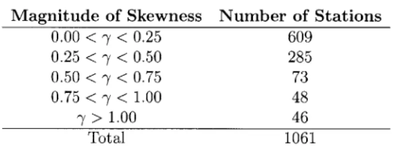
The summarized results of the network-wide analysis are shown in Table 3.2. Each station is categorized based on the magnitude of its skewness vector (derived from the East and North time series data). Table 3.2 shows that the majority of stations have low skewness values below 0.25, but that many highly skewed stations also exist in the network.
Table 3.2: Skewness in the PBO Network of GPS Stations
Magnitude of Skewness Number of Stations 0.00 < - < 0.25 609 0.25 < - < 0.50 285 0.50 < - < 0.75 73 0.75 < - < 1.00 48 7 > 1.00 46 Total 1061
Note that stations with small skewness are common, while stations with large skew-ness are relatively uncommon.
The Monte Carlo simulation described in Section 2.2 showed that at the 95% con-fidence level, the skewness of a dataset of several thousand data points described by a Gaussian noise model is between 0 and 0.2. By comparison, the PBO network of GPS stations has many stations with skewness values higher than 0.2. The distribution of skewness values shows that the noise characteristics at several hundred stations are not well-described by simple Gaussian models.
in the United States whose skewness values are greater than one. The noise charac-teristics at these stations are very poorly-described by a Gaussian model, meaning that a source of non-Gaussian error is affecting measurements at these stations. I focus on these stations with especially high skewness values during the rest of the analysis.
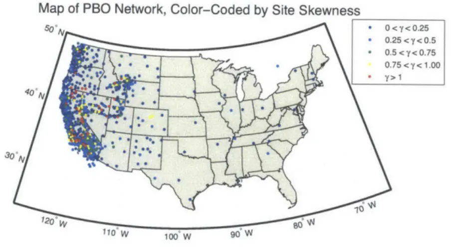
The geographic locations of all stations are shown in Figure 3-1. Based on the classifications in Table 3.2, the 609 stations with skewness between 0 and 0.25 are shown in dark blue. The next 285 stations with skewness between 0.25 and 0.50 are mapped in a lighter blue. Each successive category of skewness values has an associated color on the map. At the upper extreme, the 46 stations with the highest skewness values (y > 1) are shown in red.
Map of PBO Network, Color-Coded by Site Skewness
.' 0 0<,y< 0.25
IV .~ 0.25 < y<0.5
.* 0.5 <y< 0.75
0.75<^I< 1.00
12. 110 W 10Do, W go' W B
Figure 3-1: The PBO Network color-coded by station skewness. Red sites have the
highest values of skewness.
It is observed that all stations with the highest level of skewness are located in the western half of the United States. This observation is not particularly surprising given the high density of stations in general in the Western US. Within this region, certain locations have a higher density of highly-skewed stations than others. The Sierra Nevada, the region north of Los Angeles, and the Basin and Range Province in Nevada and Utah have large numbers of skewed stations. Regions with particularly
low skewness values, besides the Eastern United States, include the Southwest and the Central Valley of California. The Central Valley, which can be seen more clearly in Figure 3-2, has almost no highly-skewed stations. Also, the dense network of stations in Yellowstone National Park shows almost no skewness at all.
* 0 0 42.5 .* . 40.0 N 00 30.00 N * 35.0.N 3.5 N
~
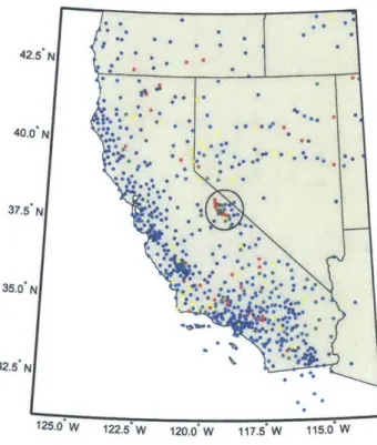
. 0 125.Ow 122.5'W 120.0*W 117.5W 115.0 WFigure 3-2: A map of the Western United States highlighting the dense region of highly-skewed stations in the eastern part of California. Another striking feature is the lack of skewed stations in the Central Valley.
One region deserves particular attention. On the eastern edge of the Sierra Nevada, highlighted in Figure 3-2, there is a region where highly-skewed stations are very common. Within the small, circled region near Mammoth Lakes, California, there are eight stations with high skewness. As this region contains a high density of skewed stations, it is an area of special interest for this project.
3.2
The Relationship Between Skewness and Local
Topography
In this section, the vector created from the skewness values was plotted on a topo-graphic map at each station. The direction of the skewness vector represents the direction in which outliers in the GPS data are most likely to occur. In many loca-tions, it appears that the direction in which GPS outliers are most likely aligns with the direction to the nearest region of high topography.
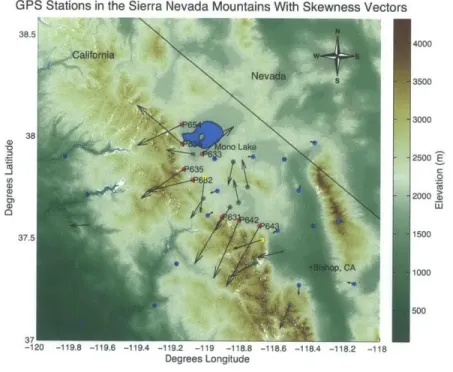
GPS Stations in the Sierra Nevada Mountains With Skewness Vectors
38.5 Nev
s
0) 37.5 .6 -119.4 -119.2 -119 -118.8 -118.6 -118.4 -118.2 -118 Degrees LongitudeFigure 3-3: Skewness vectors on a topographic map of Mammoth Lakes, California. Arrows represent the direction and magnitude of the skewness vector.
For the Mammoth Lakes region, with its high density of skewed stations, it can be observed that many of the stations have skewness vectors that point uphill from the location of the station (Figure 3-3). For example, stations P631, P642, and P643, all located to the northwest of Bishop, CA, have skewness vectors pointed in the same direction. The skewness vectors seem to point towards the high mountains to the southwest of the stations.
4000 3500 3000 2500 E 100 2000> 1500
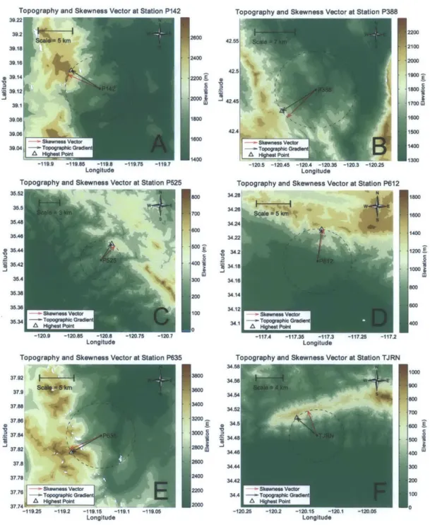
The alignment between the local uphill direction and the skewness direction is also observed at many other highly-skewed stations in the network. Figure 3-4 highlights six GPS stations and shows the close alignment between the direction of skewness and the direction of the topographic gradient at each of them. Each station in this figure has -y > 1, putting it in the category of stations with the largest skewness. In Figure
3-4, the black circle surrounding each point was used to compute the topographic gradient.
The relationship between the direction of skewness and the topographic gradient vector was quantified by finding the angle 0 between the two vectors. Small values of
O indicate a high degree of alignment between these two vectors.
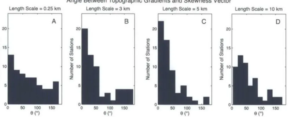
Figure 3-5 shows the values of 6 for all highly-skewed stations (-y > 1) with various
topographic gradient vectors. The topographic gradient vector was calculated at length scales of 0.25 kilometers, 3 kilometers, 5 kilometers, and 10 kilometers.
For the smallest-scale topographic gradients, at the scale of hundreds of meters, the topographic gradient seems to be uncorrelated with the direction of the skewness vector (Histogram A in Figure 3-5). The histogram only shows a slight preference for small values of 6, which represent strong alignment between the two vectors. Similarly, topographic gradients at a scale of 10 kilometers (Histogram D) show weaker correlation with the direction of the skewness vector.
At length scales of 3 to 5 kilometers, however, there is often strong alignment between the skewness vectors and the topographic gradient vectors. In Histograms B and C, the majority of the 0 values are small. This result suggests that topographic features at a scale of several kilometers can influence the direction of skewness at highly-skewed stations.
In summary, the problem of strongly skewed outliers suggests that an un-modeled source of error is affecting a specific group of GPS stations in the PBO network. Skewed outliers only appear to be a common phenomenon at 5-10% of the stations in the network. The tendency for skewed outliers is most common in mountainous regions like the Sierra Nevada and the Los Angeles area, and is less common in regions like the Eastern United States and the Central Valley of California. For highly-skewed
Topography and Skewness Vector at Station P142 39.22 39.2 5kn2 39.18 30.1 39.12 V 39.1 39.08 39.06 - Skownses Vector 39.04 -- Topographic Grad -119.9 -119.85 -119.8 -11975 -119.7 Longitude
Topography and Skewness Vector at Station P525
35.52 -V 35.42 35.4 35.38 36.38 35.36 SkownewsVctr 35.34 -Tgp SHW"h"M Pot -120.9 -120.85 -120.8 -120.75 -120.7 Longitude
Topography and Skewness Vector at Station P635
37.92 37.9 &V6 37.88 37.86 37.84 37.8 37.78 4 376 -- Skewnews Vector 3.6 -Topographic Gradient 37.74 A HOWes Point -119.25 -119.2 -119.15 -119.1 -119.05 Longitude
I
I
2400 2200 . 2= 1800 1600 1400 _j 600 700 800 400 300 200 100 0 3800 38W 3400 3200 3000 2800 200 2400 2200 2000 'II
Topography and Skewness Vector at Station P388
42.55 42.5 42.45 42.4 Sskewness Vector --Topographic Gradient SHW.hWs Point -120.5 -120.45 -120.4 -120.35 -120.3 -120.25 Longitude
Topography and Skewness Vector at Station P612
34.28 N 34.26 3424 .22 10 34.2 34.18 34.14 3412 Skownepa Vector U4.1 T'opographacreds A Highogt Point
Topography and Skewness Vector at Station TJRN
S34.5 34.48 34442 34.46 34.42 -- kwesVector 34.4 -TopographIc Grad A ihs ont -120,25 -120.2 -120.15 -120.1 -120.06 Longitude
Figure 3-4: The alignment between skewness vector and locally high topography at six
GPS stations: A) P142, Eastern Nevada; B) P388, Oregon; C) P525, Central
Califor-nia coast; D) P612, Los Angeles, CaliforCalifor-nia; E) P635, Mammoth Lakes, CaliforCalifor-nia; F)
TJRN, Santa Barbara, California. Note that the angle between the skewness vector
and the topographic gradient is small in each case.
2200 2100 2000 1600 1500 1400 1300 1800 1600 1400 1200 . 1000 800 400
I
1000 900 800 700 600 800 400 300 200 100 0 i _jLength Scale = 0.25 km 20 [j S15. 10 E z 0 50 100 150 0 ()
Angle Between Topographic Gradients and Skewness Vector
Length Scale = 3 km Length Scale = 5 km
B C 2C 1C E z 00 50 100 150 0 (*) E z 00 50 100 150 0(*) z 20- 15-10,
Figure 3-5: The relationship between topographic gradients and the skewness vector at various length scales. The histograms show distributions in the angle 0, the angle between the skewness vector and the local topographic gradient vector. The gradients at a scale of 3 to 5 kilometers are most closely aligned with the skewness vectors.
stations, the apparent alignment of the direction of the most likely GPS errors with the topographic gradient suggests that the source of the problem is somehow related to local topography at a length scale of several kilometers.
Length Scale = 10 km
D
Chapter 4
Case
Study: Outliers in the Sierra
Nevada
In this chapter, I further explore asymmetric outliers at specific stations in the Sierra Nevada and on specific days. I focus on the weather conditions that existed in the Sierra Nevada on the days with outliers.
For this case study, I focus on stations P642 and P643, two stations near Mammoth Lakes, CA. These two stations both show large skewness values and are located only about 12 kilometers apart. In each case, the preferred orientation of erroneous GPS measurements is in a direction southwest of the actual station location. The Sierra Nevada Mountains are to the southwest of the stations.
P642 and P643 both show high skewness values and are both located in the Mam-moth Lakes region, which is of interest for this project. As such, they served as prime examples for examining the effects of weather conditions on the skewness of GPS position outliers.
I focus on the relationship between position outliers and weather conditions for
Sections 4.1-4.2. In Section 4.3, I examine the patterns of phase residuals across the sky at these two stations on several days with particularly large outliers.
4.1
NWM Results
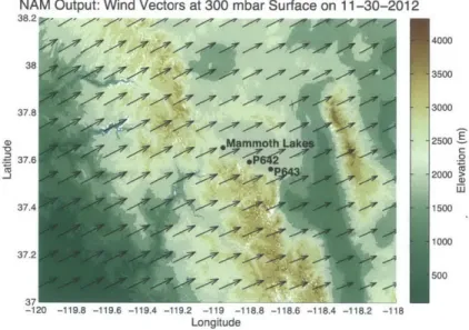
The North American Mesoscale (NAM) Numerical Weather Model (NWM) produced wind velocity fields at given levels in the atmosphere for each day of the year. As an example, the wind field on November 30, 2012 at the 300 millibar surface is shown in Figure 4-1. The wind at the 300 millibar surface above the Sierra Nevada Moun-tains was blowing from the southwest with an average velocity of 21 meters/second. The 300 millibar surface, at approximately 9 kilometers elevation, was chosen for this analysis because the velocities at this level represent the large-scale flow of the atmosphere. At this elevation, velocities are uninfluenced by boundary-layer effects and are well above the peaks of the 4-kilometer-high Sierra Nevada Mountains.
NAM Output: Wind Vectors at 300 mbar Surface on 11-30-2012
38.2 4000 38" 3500 -3000 37.8 30 37.6 42500 2000A? 37.4 1500 1000 37.2 500 -120 -119.8 -119.6 -119.4 -119.2 -119 -118.8 -118.6 -118.4 -118.2 -118 Longitude
Figure 4-1: The NAM output on November 30, 2012 for the region above Mammoth Lakes, CA. The wind vectors shown are at the 300 millibar surface, which is at approximately 9 kilometers above sea level. The average velocity is 21 m/s.
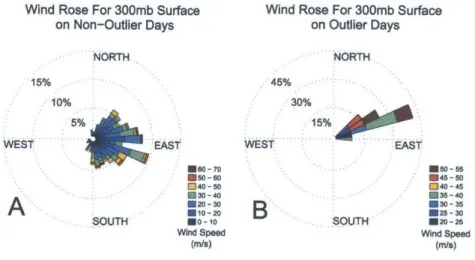
Using the NAM output, the general patterns of wind velocity near Mammoth Lakes, California were found. For each day in 2012, the NAM output at the 300 millibar surface was collected and tabulated at the grid point closest to station P643 (Figure 4-2). The dataset is displayed in the form of a wind rose, a modified histogram that displays the probabilities of winds both at a given speed and in a given direction. Plot A in Figure 4-2 shows the distribution of winds on days when the GPS data
at station P643 is normal, while Plot B shows the distribution of winds on the days with outliers that are the in largest 4% of all position deviations.
On days with typical (non-outlier) GPS measurements at station P643, the wind essentially always has a directional component blowing from west to east, which is consistent with the large-scale synoptic flow of the atmosphere over North America. Within that approximately 180 degree half-space, the range of possible wind directions is widely distributed. There is also high variability in the possible wind speeds.
However, on days with GPS outliers at station P643, the possible wind directions are restricted to a much narrower range. The winds blow from the west or the southwest on the days when outliers occur, and almost all of the outliers occur within a narrow range of about 30 degrees of direction. It can also be observed that winds on outlier days tend to have a higher magnitude than winds on non-outlier days. For example, in this dataset, there were no occurrences of outlier points on days having wind speeds below 20 m/s. An analogous plot made for station P642 shows similar results.
Wind Rose For 300mb Surface Wind Rose For 300mb Surface
on Non-Outlier Days on Outlier Days
NORTH NORTH
15% 45%
10% 30%
15%
WEST EAST WEST EAST
WOO-7o*ES-55
E50-GO 045-50
040-50 40-45
A
SOUTH Mo-1oB
SOUTH 02D -25Wind Speed Wind Speed
(m/S) (m/8)
Figure 4-2: Wind roses for the NAM-derived wind velocity estimates at 300 millibar surface above station P643. Plot A shows the wind velocities on days with non-outliers in the GPS data at station P643, and Plot B shows the wind velocities on days with outliers in the GPS data at station P643.
The direction of the upper-level winds on days with GPS outliers at these two stations is notable because it is roughly perpendicular to the ridgeline of the Sierra
Nevada Mountains. This result will be discussed further in Chapter 5.
4.2
Radiosonde Results
Radiosonde measurements provide more dense coverage in the vertical direction than NWM's, so the radiosonde observations were used to study the vertical structure of the atmosphere on days with and without errors in the GPS measurements. The radiosondes were deployed twice per day at Oakland Airport, which is located 300 kilometers east (upstream) of the stations in question. The atmospheric parameters measured by the radiosondes, especially those at higher elevations, are not likely to change very much over this length scale.
Radiosonde Wind Velocity With Height Average Wind Velocity With Height
S11000
B
9000 9000
7000 7000
5000 M 5000
3000 3000
1000 ** -Normal ~atler Days at P642 Days 1000 /Normal Days
Outli"" Days at P642
0 10 20 30 40 50 60 70 80 0 10 20 30 40 s0
Wind Speed (rn/a) Wind Speed (rn/a)
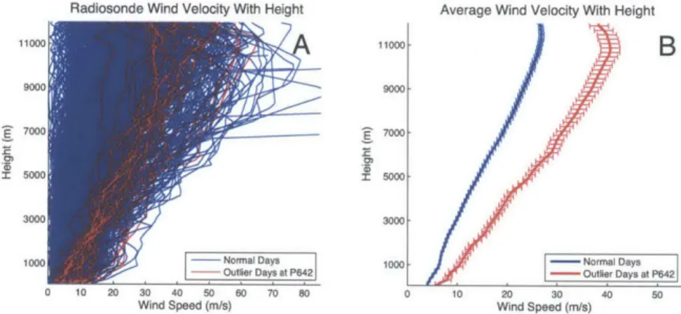
Figure 4-3: Plot A: Radiosonde-derived wind velocity as a function of elevation at Oakland during 2012. The GPS data are from station P642; red indicates that station P642 recorded an erroneous measurement within the highest 4% of its data on that day. Plot B: average wind velocity on outlier days and non-outlier days over the year. The error bars are the standard error of the mean velocity.
The primary observation from radiosonde data is that the days with outlier GPS measurements at certain stations have high wind speeds compared to the days with normal GPS position measurements (Figure 4-3). This result agrees very well with the results indicated by the NAM weather model. Furthermore, the radiosondes are able to show that this trend applies to the entire vertical profile of the wind speed above Oakland on outlier and non-outlier days.
In Figure 4-3, Plot A shows the velocity profile from each radiosonde measurement over the year. Plot B is derived from the same data and shows the average velocities on outlier days (red) and non-outlier days (blue). The error bars in Plot B are the standard deviation of each dataset divided by the square root of the number of data points in that dataset. Thus, the error bars on the figure represent the standard error of the mean velocity on days with and without GPS outliers. The error bars on the non-outlier days are smaller than the error bars on outlier days because there are many more non-outlier days in the dataset.
The amount of detail available in the vertical direction from the radiosonde data allows the Brunt-Viiisdld frequency to be calculated for each day and compared be-tween outlier days and non-outlier days (Figure 4-4). As in Figure 4-3, the error bars represent the standard error of the mean Brunt-Vdisdld frequency on days with and without GPS outliers. The GPS station is station P642.
Average Brunt-VdistIl Frequency at Oakland on Normal Days and Outlier Days
11000 Normal Days at P642 --- Outlier Days at P642 9000 E 7000 5000 3000-1000 0.006 0.008 0.01 0.012 0.014 0.016 0.018 0.02 Brunt-Vdisdl& Frequency (s-)
Figure 4-4: The average Brunt-Viisdld frequency as measured from Oakland Airport during the year 2012. The red curve represents the average Brunt-Vdisdld frequency on days when station P642 recorded erroneous measurements within the highest 4% of its data.
It is notable that on outlier days, the average Brunt-Vdisdld frequency is higher than normal between 3 and 7 kilometers elevation. On the same days, it is lower than
normal above 8 kilometers elevation. Since the Brunt-Vdisild frequency is related to the stability of the atmosphere, this result shows that the atmosphere has higher-than-average stability between 3 and 7 kilometers elevation on days with GPS outliers.
The atmosphere also shows lower-than-average stability above 8 kilometers elevation on days with GPS outliers. This result will be discussed further in the context of lee waves in Chapter 5.
4.3
MODIS Results
A survey of MODIS images over California shows that lee waves to the east of the
Sierra Nevada can be visually observed in satellite imagery on many of the days in which GPS outliers occur. In the images, the lee waves appear as closely-spaced rows of clouds parallel to the mountain range. The linear cloud formations show between two and ten wavelengths of lee waves.
Figure 4-5: Lee waves in the Sierra Nevada on March 13, 2012, as observed by the MODIS instrument on NASA's Terra satellite.
day when station P642 recorded a large outlier of 10.69 millimeters in the south-west direction (Figure 4-5). Interestingly, P643 recorded a displacement of only 1.28 millimeters on the same day. In the MODIS image, more than ten wavelengths of lee waves are visible downstream of Mammoth Lakes, CA. Based on this image, the wavelength of the lee waves was measured to be about 15 kilometers.
The occurrence rate of lee waves, as determined by a year-long survey of the
MODIS image archive, is shown in Table 4.1. In general, lee waves appear in the MODIS images approximately one out of six days of the year.
However, the occurrence rate of lee waves in the MODIS images is much higher on days when stations P642 and P643 record outliers in the GPS data. On these days, lee waves are observed approximately two-thirds of the time.
Table 4.1: Lee Wave Observations from MODIS Satellite Imagery
Data set Total number of days Lee wave days
All days in 2012 366 63
Outlier days at P642 18 12
Outlier days at P643 18 11
4.4
Phase Residual Results
The phase residuals for P642 and P643 were analyzed on March 27, 28, and 29, 2012. Stations P642 and P643 each recorded position outliers during this period, but the largest outliers occurred on different days at these two stations. In MODIS images, lee waves were observed above the Sierra Nevada on all three of these days.
In the following plots, the phase residuals, which were originally dimensionless differences in phase, are multiplied by the wavelength of GPS signals (19 centimeters) in order to be expressed in millimeters. The phase residuals are shown as sky maps from the perspective of the receiver, so the East and West directions are opposite what they would be in normal plan-view.
Tens of thousands of individual GPS measurements are recorded daily at every station, each with an associated phase residual. The following maps show the local