HAL Id: hal-00305081
https://hal.archives-ouvertes.fr/hal-00305081
Submitted on 9 Jul 2007
HAL is a multi-disciplinary open access
archive for the deposit and dissemination of
sci-entific research documents, whether they are
pub-lished or not. The documents may come from
teaching and research institutions in France or
abroad, or from public or private research centers.
L’archive ouverte pluridisciplinaire HAL, est
destinée au dépôt et à la diffusion de documents
scientifiques de niveau recherche, publiés ou non,
émanant des établissements d’enseignement et de
recherche français ou étrangers, des laboratoires
publics ou privés.
A multimodel ensemble approach to assessment of
climate change impacts on the hydrology and water
resources of the Colorado River Basin
N. S. Christensen, D. P. Lettenmaier
To cite this version:
N. S. Christensen, D. P. Lettenmaier. A multimodel ensemble approach to assessment of climate
change impacts on the hydrology and water resources of the Colorado River Basin. Hydrology and
Earth System Sciences Discussions, European Geosciences Union, 2007, 11 (4), pp.1417-1434.
�hal-00305081�
www.hydrol-earth-syst-sci.net/11/1417/2007/ © Author(s) 2007. This work is licensed under a Creative Commons License.
Earth System
Sciences
A multimodel ensemble approach to assessment of climate change
impacts on the hydrology and water resources of the
Colorado River Basin
N. S. Christensen and D. P. Lettenmaier
Department of Civil and Environmental Engineering Box 352700, University of Washington, Seattle WA 98195, USA Received: 16 November 2006 – Published in Hydrol. Earth Syst. Sci. Discuss.: 13 December 2006
Revised: 27 April 2007 – Accepted: 5 June 2007 – Published: 9 July 2007
Abstract. Implications of 21st century climate change on the hydrology and water resources of the Colorado River Basin were assessed using a multimodel ensemble approach in which downscaled and bias corrected output from 11 General Circulation Models (GCMs) was used to drive macroscale hydrology and water resources models. Downscaled cli-mate scenarios (ensembles) were used as forcings to the Variable Infiltration Capacity (VIC) macroscale hydrology model, which in turn forced the Colorado River Reservoir Model (CRMM). Ensembles of downscaled precipitation and temperature, and derived streamflows and reservoir system performance were assessed through comparison with current climate simulations for the 1950–1999 historical period. For each of the 11 GCMs, two emissions scenarios (IPCC SRES A2 and B1, corresponding to relatively unconstrained growth in emissions, and elimination of global emissions increases by 2100) were represented. Results for the A2 and B1 cli-mate scenarios were divided into three periods: 2010–2039, 2040–2069, and 2070–2099. The mean temperature change averaged over the 11 ensembles for the Colorado basin for the A2 emission scenario ranged from 1.2 to 4.4◦C for
peri-ods 1–3, and for the B1 scenario from 1.3 to 2.7◦C.
Precip-itation changes were modest, with ensemble mean changes ranging from −1 to −2% for the A2 scenario, and from +1 to
−1% for the B1 scenario. An analysis of seasonal
precipita-tion patterns showed that most GCMs had modest reducprecipita-tions in summer precipitation and increases in winter precipitation. Derived April 1 snow water equivalent declined for all en-semble members and time periods, with maximum (ensem-ble mean) reductions of 38% for the A2 scenario in period 3. Runoff changes were mostly the result of a dominance of increased evapotranspiration over the seasonal precipitation shifts, with ensemble mean runoff changes of −1, −6, and
Correspondence to: D. P. Lettenmaier
(dennisl@u.washington.edu)
−11% for the A2 ensembles, and 0, −7, and −8% for the
B1 ensembles. These hydrological changes were reflected in reservoir system performance. Average total basin reser-voir storage and average hydropower production generally declined, however there was a large range across the ensem-bles. Releases from Glen Canyon Dam to the Lower Basin were reduced for all periods and both emissions scenarios in the ensemble mean. The fraction of years in which short-ages occurred increased by approximately 20% by period 3 for both emissions scenarios.
1 Introduction
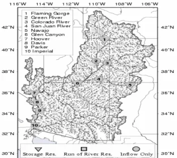
The Colorado River Basin (CRB) includes parts of seven U.S. states and Mexico (Fig. 1). The headwaters lie in the Rocky Mountains of Wyoming and Colorado, from which the river flows some 1400 km to the Gulf of California. It drains a mostly semi-arid region, with an average of only 40 cm/year of precipitation over the 630 000 km2basin. 70% of the Colorado’s flow originates as snowmelt, with the annual hydrograph dominated by winter accumulation and spring melt. 85% of streamflow is generated from 15% of the area, while the lower basin (below Lees Ferry, AZ) con-tributes only 8% of the annual streamflow. The Colorado River also has considerable temporal variability, with a co-efficient of variation for annual streamflow of .33 (by com-parison, the coefficient of variation for the Columbia River is less than 0.2). From 1906–2003, annual streamflow had a minimum, maximum, and mean of 6.5, 29.6 and 18.6 billion cubic meters (BCM) at Lees Ferry. A recent 500-year recon-struction of Colorado River discharge using tree ring data (Woodhouse et al., 2006) suggests that the long term aver-age annual flow is somewhat lower than for the 1906–2003 reference period – in the range 17.7–18.1 BCM.
Fig. 1. Colorado River Basin with 1/8 degree VIC routing network
and major system reservoirs.
The Colorado River is often described as the most regu-lated and over allocated river in the world (USDOI, 2000). It has an aggregate reservoir capacity of 74.0 BCM, four times its mean annual flow. 85% of basin storage capacity lies in Lakes Powell (formed by Glen Canyon Dam) and Mead (formed by Hoover Dam). The Law of the River which gov-erns management of the river consists of 12 major and many minor federal and state laws, treaties, court decisions, and compacts and divides the basin’s water between the Upper Basin states (Wyoming, Utah, Colorado, and New Mexico), Lower Basin states (Arizona, Nevada, California), and Mex-ico. The first document of the Law of the River is the Col-orado Compact of 1922 which after gauging the river during a period of abnormally high flow apportioned 9.3 BCM/yr to both the Upper and Lower Basin. Another element of the Law of the River is the U.S.-Mexico Treaty of 1944 which stipulates that Mexico will receive 1.9 BCM/yr on average at the U.S. – Mexico border. During most of the period since the signing of the compact the 10 year average flow has been below the 20.5 BCM that has been allocated (see Fig. 2) – a situation that is further exacerbated by the estimated 1– 2 BCM of annual reservoir evaporation. On the other hand, the Compact allocation to the upper basin states has to date not been fully utilized, and for this reason the Law of the River has been able to function notwithstanding the apparent overallocation of the river’s water.
The hydrologic implications of climate change are a global concern (Milly et al., 2005), but the CRB is especially vul-nerable due to the sensitivity of discharge to precipitation and temperature changes (both of which affect snow accu-mulation and melt patterns as well as evapotranspiration), ef-fects which are exacerbated by the semi-arid nature of the
0 5 10 15 20 25 30 35 1905 1915 1925 1935 1945 1955 1965 1975 1985 1995 2005 A n n u a l F lo w ( B C M )
Annual Flow at Imperial Dam Running Mean at Imperial Dam 10 Year Running Mean at Imperial Dam
Fig. 2. Annual, 10 year average and running average of natural flow
at Imperial Dam, AZ.
basin (Loaiciga, 1996). Global General Circulation Mod-els (GCMs) of the coupled land-ocean-atmosphere system project an increase in global mean surface air temperature be-tween 1.8◦C and 5.4◦C between 1990 and 2100 yet disagree
upon the tendency and seasonality of precipitation changes (IPCC, 2001) and their spatial distribution regionally. In gen-eral, increases in temperature within the CRB will increase the rain to snow ratio, move runoff peaks earlier in the spring, increase evapotranspiration, and decrease annual streamflow, whereas precipitation changes will primarily affect annual streamflow volume (Christensen et al., 2004). The season-ality of precipitation changes, however, contribute to runoff changes as well: a greater percentage of winter precipitation generates runoff than in summer (due to lower evaporative demand).
A previous study of potential climate change in the CRB (Christensen et al., 2004) used the U.S. Department of En-ergy/National Center for Atmospheric Research Parallel Cli-mate Model (PCM) with a business-as-usual (BAU) global emission scenario (the most recent GCM runs performed for IPCC (2007) no longer use a BAU scenario, however the A2 scenario used in the results we report here is the closest to BAU of those considered). In Christensen et al (2004), aver-age temperature changes of 1.0, 1.7, and 2.4◦C and
precipi-tation changes of −3, −6, and −3% were predicted for the CRB for periods 2010–2039 (period 1), 2040–2069 (period 2), and 2070–2099 (period 3), respectively, relative to 1950– 1999 means. These temperature and precipitation changes led to reductions of April 1 snow water equivalent (SWE) of 24, 29, and 30% and runoff reductions of 14, 18, and 17% for periods 1–3. Other studies (Gleick, 1987; Lettenmaier et al., 1992; Nash and Gleick, 1991, 1993; Hamlet and Letten-maier, 1999; McCabe and Hay, 1995; McCabe and Wolock, 1999; Wilby et al., 1999; Wolock and McCabe, 1999) of cli-mate change impacts on hydrology and water resources of western U.S. river basins have used both climate signals from
GCMs as well as prescribed temperature and precipitation changes. All studies have assumed or predicted increasing temperatures, but have disagreed upon both the magnitude and direction of precipitation changes. Aside from Chris-tensen et al. (2004), only one of these studies (Nash and Gleick, 1991, 1993) has been specific to the CRB. Nash and Gleick assessed the impacts of a doubling of CO2
concentra-tions (at the time of their study, so-called transient GCM out-put was not widely available). In addition, Nash and Gleick (1991) evaluated prescribed changes of +2◦C and +4◦C
cou-pled with precipitation reductions of −10% and −20%. The 2◦C increase/10% precipitation decrease resulted in a 20%
streamflow reduction while the 4◦C increase/20%
precipita-tion decrease resulted in a 30% runoff decrease. A related study by Nash and Gleick (1993) which analyzed scenarios with both increases and decreases in precipitation suggested that slight increases in precipitation would be offset by in-creased evapotranspiration, with the net result being reduc-tions in streamflow ranging from 8 to 20%. Wolock and Mc-Cabe (1999) utilized climate output from GCMs to drive a hydrology model and concluded that a slight increase in pre-cipitation with modest temperature increase would result in decreased streamflow, while for another GCM a significant increase in precipitation coupled with a larger temperature increase would result in increased streamflow. The diversity of scenarios considered by the assortment of climate change studies reflects the considerable uncertainty in the expected amount of warming and in the magnitude and direction of potential precipitation changes.
The managed water resources of the CRB are highly sen-sitive to runoff reductions due to the almost complete allo-cation of streamflow to consumptive uses. The past studies suggest that increased temperature alone, unless offset by in-creases in precipitation, will stress the water resources of the CRB, while any precipitation decrease will exacerbate these stresses. Nash and Gleick (1993) found reservoir system storage was highly sensitive to changes in runoff, suggest-ing that the system is currently in a rather fragile balance. Christensen et al. (2004) found that runoff reductions of 14– 18% resulted in system storage reductions of 30–40% and target releases from Glen Canyon Dam being met 17–32% less often than in the reference (1950–1999) historic period. Nash and Gleick (1993) found that violations of the Com-pact would occur if average runoff dropped by only 5%. On the one hand, the large storage to runoff ratio of the basin mitigates the effects of seasonal shifts in runoff timing asso-ciated with a warmer climate; even though the large storage capacity will have little effect on long term reliability of wa-ter deliveries if average flows decline.
The present study utilizes 11 GCMs under IPCC Special Report on Emission Scenarios (IPCC, 2000) emission sce-narios A2 and B1, where A2 corresponds to relatively un-constrained growth in global emissions, and B2 corresponds to elimination of global emissions increases by 2100. Each GCM’s historical simulation was used to bias correct and
downscale the temperature and precipitation signals from the A2 and B1 scenarios using methods outlined in Wood et al. (2002) and Wood et al. (2004). The bias corrected and downscaled temperature and precipitation signals were then used to drive the Variable Infiltration Capacity (VIC) macroscale hydrology model (Liang et al., 1994; Nijssen et al., 1997) at a daily time step. Monthly aggregates of VIC-simulated streamflow at selected reservoir inflow points (Fig. 1) were used to force the CRRM. CRRM, described in more detail in Christensen et al. (2004) is a simplified version of the Colorado River Simulation System (USDOI, 1985). It predicts storage in the main CRB reservoirs, and deliveries of water to major water users, as well as hydropower gen-eration. We summarize results of both the VIC and CRRM simulations for period 1 (2010–2039), period 2 (2040–2069, and period 3 (2070–2099), and compare them with a “histor-ical” simulation driven by 1950–1999 observations.
2 Approach
2.1 General circulation models and emission scenarios The 11 GCMs which produced the climate scenarios used in this study are summarized in Table 1, which includes ref-erences to the details of each model. Although many other GCM runs were prepared for the IPCC Fourth Assessment Report (AR4; IPCC, 2007), these 11 model runs are the most consistent in terms of the future simulation period (all were run for at least the period 2000–2100), and the emissions sce-narios used. These GCMs represent the major global mod-eling centers and provide the basis for the most thorough climate study of the CRB to date. In that respect, we note that our approach here is a generalization of Christensen et al. (2004), who ran one model and emissions scenario for the CRB using essentially the same methods as were used in this study, and Maurer (2007), who ran 10 of the same 11 models we use, and the same emissions scenarios for California.
For its Fourth Assessment Report, the IPCC created six plausible global greenhouse gas emissions scenarios; A1F, A1B, A1T, A2, B1, and B2. With respect to global emissions of greenhouse gases (and hence, in general, global average temperature increases) from warmest to coolest are scenar-ios A1FI, A2, A1B, B2, A1T, and B1. The A2 and B1 sce-narios were chosen for this study because they are the most widely simulated over all models (not all modeling groups have archived runs for all emissions scenarios), and because they represent a plausible range of conditions over the next century.
In the A2 scenario, global average CO2 concentrations
reach 850 ppm by 2100, while in the B1 scenario CO2
con-centrations initially increase at nearly the same rate as in the A2 scenario, but then level off around mid-century and end at 550 ppm by 2100 (IPCC, 2000). Christensen et al. (2004) used Parallel Climate Model (PCM) runs with the BAU
Table 1. General Circulation Models used to produce scenarios assessed in this study.
Abbreviation Modeling Group/Country IPCC Model ID Reference
CNRM Centre National de Recherches M´et´eoroliques, France CNRM-CM3 Salas-M´elia et al. (2006)
CSIRO CSIRO Atmospheric Research, Australia CSIRO-Mk3.0 Gordon, H. B. et al. (2002)
GFDL Geophysical Fluid Dynamics Laboratory, USA GFDL-CM2.0 Delworth et al. (2006)
GISS Goddard Institute for Space Studies, USA GISS-ER Russell et al. (1995, 2000)
HADCM3 Hadley Center for Climate and Prediction and Research, UK UKMO-HadCM3 Gordon et al. (2002)
INMCM Institute for Numerical Mathematics, Russia INM-CM3.0 Diansky and Volodin (2002)
IPSL Institut Pierre Simon Laplace, France IPSL-CM4 IPSL (2005)
MIROC Center for Climate Systems Research, Japan MIROC3.2 K-1 model developers (2004)
MPI Max Planck Institute for Meteorology, Germany ECHAM5/MPI-OM Jungclaus et al. (2006)
MRI Meteorological Research Institute, Japan MRI-CGCM2.3.2 Yukimoto et al. (2001)
PCM U.S. Department of Energy/ PCM Washington et al. (2000)
National Center for Atmospheric Research, USA
emissions scenario which as noted above is most compara-ble to A2 of the emissions scenarios used in IPCC AR4.
Details of the bias correction and downscaling approach used to translate GCM output into VIC input are reported in Wood et al. (2002, 2004) and Maurer (2007). In brief, the method downscales monthly simulated and observed tem-perature and precipitation probabilities at the GCM spatial scale (regridded to a common 2 degrees latitude by longitude spatial resolution) to the 1/8 degree resolution at which the VIC hydrology model was applied through use of a probabil-ity mapping procedure that is “trained” to monthly empirical probability distributions of the climate model output for cur-rent climate conditions to equivalent space-time aggregates of the gridded (one-eighth degree spatial resolution) obser-vation set of Maurer et al. (2002). The climate model signal was then temporally and spatially disaggregated through use of a resampling approach to create a daily forcing time series for the hydrology model at the same one-eighth degree spa-tial resolution. This method facilitates investigation of the implications of the true transient nature of climate warming as opposed to the more common methods employed where decadal temperature and precipitation shifts are averaged to give a step-wise evolution of climate (e.g. Hamlet and Letten-maier, 1999). It should be noted that the bias correction and downscaling technique that we used by construct reproduce observed climatologies in the special case where the GCM runs have no precipitation and temperature change.
2.2 VIC model application to the CRB
Liang et al. (1994) and Nijssen et al. (1997) provide de-tails of the VIC model and its application to continental river basins, while Christensen et al. (2004) provide details of its application to the CRB, hence our description here is highly condensed. VIC is a grid cell based macroscale hydrology model that typically runs at spatial resolutions ranging from one-eighth to two degrees latitude by longitude. The VIC model is forced by gridded temperature, precipitation, and
wind time series, as well as other surface radiative and me-teorological variables that are derived from daily mean tem-perature and temtem-perature minima/maxima following meth-ods outlined by Maurer et al. (2002). The VIC model can be run either at a sub-daily time step which facilitates a full en-ergy balance, or (as was used in this study) at daily time step in water balance mode. The model simulates soil moisture dynamics, snow accumulation and melt, evapotranspiration, and generates surface runoff and baseflow which are subse-quently routed through a grid based river network to simulate streamflow at selected points within the basin.
As in Christensen et al. (2004), VIC grid cell runoff was routed to locations representing the inflow to seven major reservoirs and three inflow-only locations used in the reser-voir simulation model (Fig. 1). VIC was calibrated by forc-ing the model with historic climate observations and ad-justing parameters that govern infiltration and base flow re-cession to match simulated streamflow with naturalized ob-served obtained from the U.S. Bureau of Reclamation (2000) at selected points for the same period of record. The over-lapping period of record between the Maurer et al. (2002) data set (and therefore historic simulated streamflow) and ob-served naturalized streamflow is 1950–1999, during which VIC cumulative simulated streamflow was 768 BCM and ob-served naturalized streamflow was 776 BCM. This represents a VIC bias to slightly underpredict streamflow (by about one percent). The relative biases at Green River, UT and the Colorado River near Cisco, UT, were slightly larger (3 and
−9%, respectively). The additional step of first bias
correct-ing these streamflows before drivcorrect-ing CRRM with them was added; this is a step that was not included in the Christensen et al. (2004) study. Snover et al. (2003) provide details, but this step essentially maps between simulated and observed probability distributions at each CRRM inflow point in each calendar month during the overlapping 1950–1999 period. This same relationship is then applied to the future GCM runs, therefore eliminating any systematic spatial bias.
2.3 CRRM implementation
CRRM is a simplified version of the U.S. Bureau of Reclamation’s (USBR) Colorado River Simulation System (CRSS) (Schuster, 1987; USDOI, 1985) developed by Chris-tensen et al. (2004) for assessment of the affects of altered streamflow regimes on performance of the Colorado River reservoir system. CRRM is driven by naturalized streamflow (VIC output) at the inflow points shown in Fig. 1. It repre-sents all major physical water management structures in the CRB. Pre-specified operating policies are used to simulate reservoir levels and releases, hydropower production, and di-versions on a monthly time step.
Because of the large fraction of total CRB reservoir stor-age in Lakes Powell and Mead, not all of the physical or operational complexities of the river system need to be repre-sented in CRRM to enable the assessment of climate change implications of reservoir system performance. CRRM there-fore represents the CRB reservoir system with four storage and three run-of-the-river reservoirs. The storage reservoirs are Flaming Gorge, Navajo, Lake Powell, and Lake Mead, of which only Lakes Powell and Navajo are essentially equiva-lent to the true reservoirs. Flaming Gorge includes the age capacity of Fontenelle and Lake Mead includes the stor-age capacity of the downstream reservoirs that are treated as run-of-the-river in CRRM. Hydropower is simulated at all reservoirs except Navajo and Imperial.
As noted above, the operating policies of the CRB reser-voir system are dictated by the Law of the River. In CRRM, like CRSS, these laws have been simplified so that the main regulations affecting operations are a mandatory release of 10.2 BCM per year from Glen Canyon Dam (for the Lower Basin’s 9.2 BCM/yr entitlement and one-half of Mexico’s 1.9 BCM/yr) and an annual release from the Lower Basin to Mexico of 1.9 BCM. CRRM, again like CRSS, requires the release from Lake Powell regardless of the reservoir level rel-ative to its minimum power pool; only when it is not physi-cally possible to release water (dead storage) are releases to the Lower Basin curtailed. CRRM shortage delivery opera-tions were updated in CRRM relative to the version of the model used in Christensen et al. (2004) to reflect the “basin states alternative” (BSA) which is likely to be adopted as the basis for water deliveries in the future. The BSA has three different shortage levels (494, 617, and 740 MCM/yr that are imposed at Lake Mead elevations of 327.66, 320.05, and 312.42 m, respectively. The BSA also stipulates a hard protect of the Southern Nevada’s Water Authority (SNWA) intake at an elevation of 304.80 m. At this elevation deliv-eries to the lower basin will be reduced, to zero if need be, to ensure no further reduction of elevation. The first three reductions are weighted 79% to CAP, 17% to Mexico, and 4% to SNWA. The BSA does not stipulate how shortages are allocated after the 740 MCM/yr level; however CRRM fol-lows the Law of the River and recognizes CAP’s allocation to be junior to the MWD, which in turn is junior to the
Im-perial Irrigation District (IID). CRRM, like CRSS, does not impose shortages on the Upper Basin but rather passes them onto the Lower Basin even though this could be considered a violation of the Law of the River (Hundley, 1975).
Water demands in this study were based on the USBR’s Multi-Species Conservation Program (MSCP) (USDOI, 2000) baseline demands for year 2000. Upper Basin de-mands were fixed at 5.2 BCM/yr and Lower Basin at their full entitlement of 9.2 BCM/yr. Although demands will likely in-crease as population inin-creases in the basin, holding demands steady allows us to isolate the effects climate change from the confounding effects of transient demand increase. CRRM represents withdrawals from the river at 11 diversion points, each of which has a unique monthly return ratio (fraction of water diverted that is returned to the river). If there is in-sufficient water within a river reach or reservoir to meet a demand, the two upstream reservoirs are allowed to make releases to fulfill the demand. Present perfected water rights are not explicitly modeled in CRRM, instead priority is given to upstream users except in the case of Lower Basin short-ages.
Christensen et al. (2004) provide validation plots of CRRM during the period 1970–1990, in which it had a 1% monthly storage error and a 0% accumulated error over the 20 year period. During this period it had a 12% accumu-lated hydropower error, but the error was largely due to the high reservoir levels in the mid-80s coupled with CRRM’s lack of inflow forecasting. Given results reported in the fol-lowing section, it appears unlikely that these high reservoir levels will be reached in the future, so CRRM arguably rep-resents hydropower production adequately for the purpose of this study.
3 Results
In this section we analyze downscaled and bias corrected GCM climate scenarios (using the method of Wood et al, 2004) which we compare to 1950–1999 gridded histori-cal observations of daily temperature and precipitation from Maurer et al. (2002). Hydroclimatic variables (runoff, SWE, evaporation) simulated by VIC for the GCM scenarios are compared to VIC simulations driven by the 1950–1999 cli-mate observations. Baseline statistics for the 1950–1999 pe-riod are termed “historical”, while GCM results are divided into period 1 (2010–2039), period 2 (2040–2069), and period 3 (2070–2099). We discuss in this section ensemble means and quartiles (which, taken together, give an idea of the range of the resuls), whereas more detailed results for individual GCMs and emission scenarios are reported in Appendix A.
Figure 3
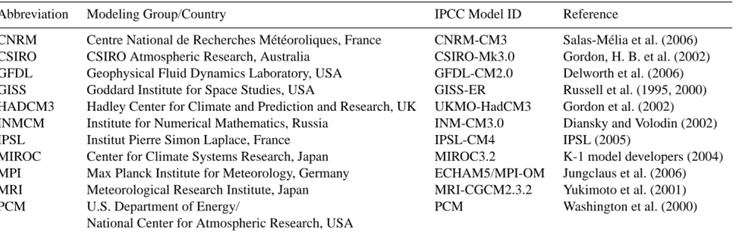
Fig. 3. Basin averaged temperature change for SRES A2 and B1
emission scenarios.
3.1 Downscaled climate change scenarios
Figure 3 shows the transient basin average temperature for each of the 11 GCMs throughout the 21st century under both the A2 and B1 emission scenarios. Although there is consid-erable spread within each scenario, it is apparent that by the second half of the century there is significantly more warm-ing associated with the A2 than the B1 scenario. By period 2, all the climate models with the exception of PCM simulate warmer temperatures for the A2 scenario, and by period 3 all GCMs simulate warmer A2 temperatures (average warming of 2.7◦C in B1 vs. warming of 4.4◦C in the A2 scenario).
Ta-ble 2 summarizes ensemTa-ble average changes while TaTa-bles A1 and A2 report results for individual ensemble members.
Figure 4 shows the shift in annual distribution of temper-ature and precipitation, and resulting runoff for periods 1–3 relative to the 1950–1999 historic simulation. Results are presented for the ensemble average and 1st and 3rd quar-tiles. As expected (because A2 and B1 emission scenarios are similar for the first part of the century) there is little dif-ference in warming between the two scenarios during period 1. The ensemble average B1 period 1 warming is 1.28◦C
(1st and 3rd quartiles 1.02 and 1.67◦C) while A2 is 1.23◦C
(0.95, 1.49◦C). By period 2 the B1 scenario has a mean shift
of 2.05◦C (1.64, 2.48◦C). In the same period, the mean A2
shift is 2.56◦C (1.94, 2.83◦C). By period 3, scenario A2 is
1.7◦C warmer than B1. B1 has a mean shift of 2.74◦C (1.89,
3.23◦C) while A2 is 4.35◦C (3.32, 5.38◦C). The ensemble
averages for all scenarios and time periods have more warm-ing from mid-summer to early fall, which may be attributable to fact that there is less moisture during these months than in the historical simulation, and therefore more energy going to sensible than to latent heating.
Fig. 4. Changes in annual average temperature, precipitation, and
runoff for periods 1, 2, and 3 for SRES scenarios A2 and B1.
Averaged over all GCMs (“ensemble average”), changes in average annual precipitation are −1 (−6, +3), −2 (−7, +7), and −2 (−8, +5)% for the A2 scenario, and +1 (−3, +6), −1 (−6, +4), and −1 (−8, +2)% for the B1 emission scenario for periods 1–3, respectively (Fig. 5). Although the trend is for very slight decreases in the ensemble mean pre-cipitation, and hence runoff decreases are driven primarily by increased evapotranspiration, there are ensemble mem-bers where increased precipitation offsets increased evapo-rative losses resulting in increased runoff. The number of ensemble members with this character in general decreases with time for both emissions scenarios (see Appendix A for individual ensemble member results). Also, although annual precipitation decreases very slightly in the annual mean, en-semble average winter precipitation increases (Fig. 4b). The increase in winter (October–March) precipitation is 5, 1, and 2% for the B1 scenario, and 6, 5, and 4% for the A2 sce-nario for periods 1–3, respectfully. Upstream of Lees Ferry (where a larger percentage of precipitation results in runoff), the B1 scenario has a 7% winter precipitation increase in pe-riod 1 and 6 and 8% increases in pepe-riods 2 and 3. In the A2 scenario, the increase in winter precipitation upstream of Lees Ferry is 8, 10, and 14% in periods 1–3, respectively. In section 3.4 we perform a separate sensitivity analysis of the implications of these changes, but in short, a shift towards winter precipitation results in more runoff for a given pre-cipitation amount. These increases in winter prepre-cipitation
Fig. 5. Annual average precipitation changes for periods 1–3
rela-tive to 1950–1999 historic simulation.
amounts are opposite to the projections by the earlier version of PCM utilized in Christensen et al. (2004). The ensem-ble averages in that study had winter precipitation decreases of 4, 6, and 4% for periods 1–3, respectfully, which drove much larger reductions in (annual) streamflow than projected in this study (see below).
Figure 5 shows the spatial distribution of predicted changes in annual precipitation. Increases are predomi-nantly in the high elevation areas of the Rockies in Colorado, Wyoming and Utah while decreases are greatest in the desert portions of the southeast basin in Arizona and New Mexico. It should be noted that the fine spatial resolution of the pre-dicted precipitation changes in Fig. 5 is in fact driven by the coarse spatial resolution of the GCM output. The regions in Fig. 5 that show the greatest precipitation increases are in general the areas that have high precipitation in the same months for which the GCMs predict increases. The moun-tainous headwaters regions, for example, receive a prepon-derance of their precipitation in the winter, and because the GCMs on average have winter precipitation increases, the mountain headwaters have the greatest annual average pre-cipitation increases. The converse holds for summer; de-creases in basin wide summer precipitation cause the greatest annual (volume) reductions to occur in the southeast since this region receives most of its rainfall during the summer months.
3.2 Runoff changes
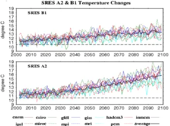
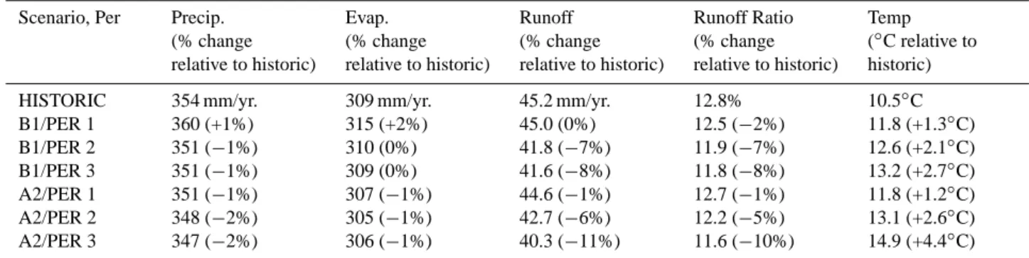
Figure 6a shows spatial changes in the ensemble average mean annual runoff for periods 1–3 relative to simulated his-toric, and Fig. 6b shows the mean monthly hydrograph for three streamflow locations in the basin. 1950–1999 basin average annual precipitation is 354 mm, of which 310 mm evaporates, leaving 45 mm to runoff. This constitutes a runoff ratio of around 13% which is typical of semi-arid
wa-Fig. 6. (a) Spatial distribution of predicted (ensemble mean)
changes in mean annual runoff for periods 1–3 relative to simulated historic, and, (b) mean monthly hydrograph for the Green River at Green River, UT, Colorado River near Cisco, UT, and Colorado River below Imperial, AZ for simulated historic discharge, and en-semble means for Periods 1–3.
tersheds (Nash and Gleick,, 1991). Runoff stays essentially unchanged in period 1 for both SRES scenarios, decreases by 7 (−15, 0) and 6 (−14, +8)% in period 2 for the B1 and A2 scenarios, respectively, and by 8 (−18, −1) and 11 (−16, −1)% in period 3 for the B1 and A2 scenario. Ta-ble 2 shows average annual precipitation, evaporation, and runoff in mm/year, and runoff ratio and basin average an-nual temperature. Although precipitation changes are mod-est (+1– −2%), changes (mostly decreases) in runoff ratio are larger. The runoff ratio reductions are driven both by temperature (the higher the temperature, the lower the runoff ratio) as well as by shifts in the seasonality of precipita-tion (see Sect. 3.4). For individual GCM ensemble mem-bers in which there are comparable temperature and precipi-tation changes, the runs that have larger shifts towards win-ter precipitation have higher runoff ratios. In Christensen et al. (2004) we utilized an earlier version of PCM which projected slightly greater precipitation decreases, smaller temperature increases, and from which substantially larger runoff decreases were inferred. For period 3 annual average temperature increases of 2.4◦C and precipitation decreases
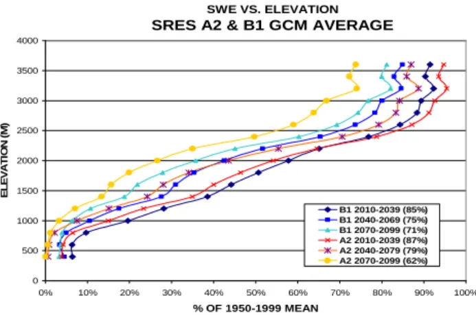
SWE VS. ELEVATION
SRES A2 & B1 GCM AVERAGE
0 500 1000 1500 2000 2500 3000 3500 4000 0% 10% 20% 30% 40% 50% 60% 70% 80% 90% 100% % OF 1950-1999 MEAN E L E V A T IO N ( M ) B1 2010-2039 (85%) B1 2040-2069 (75%) B1 2070-2099 (71%) A2 2010-2039 (87%) A2 2040-2079 (79%) A2 2070-2099 (62%)
Fig. 7. Changes in annual average snow water equivalent “present”
by elevation for periods 1–3 relative to simulated historical.
large runoff decrease for the modest temperature and precip-itation change (relative to the ensemble means in this study) is a result in large part of the earlier PCM’s shift away from winter precipitation.
Although a reduction of 5 mm/year of runoff may seem modest, it represents a reduction of 11% which has major im-plications on a system whose water is already over-allocated. 3.3 Snowpack changes
Basin average April 1 snow water equivalent (SWE), the depth of water that the snowpack would produce if melted, declines by 13 (25, 6), 21 (29, 16), and 38 (48, 19)% in sce-nario A2, and by 15 (24, 11), 25 (31, 18), and 29 (33, 19)% in scenario B1 in periods 1–3, respectively. Winter precipi-tation is greater for all ensemble means relative to the histor-ical period, leading to the conclusion that the reductions in SWE are directly attributable to higher winter temperatures and the resulting decrease in the ratio of precipitation falling as snow vs. rain. Reductions in SWE present are greatest in the low to mid elevation transitional zone (Fig. 7). The met-ric “snow present” is a function of both SWE depth and the amount of time the SWE is present. If an equivalent amount of snow falls, but melts twice as fast, it is considered 50% of historical. These results are consistent with Nash and Gle-ick (2003), Wilby et al. (1999), McCabe and Wolock (1999), Brown et al. (2000), and Christensen et al. (2004).
3.4 Sensitivity of runoff to seasonality of precipitation A separate analysis was performed to better understand the effect that a seasonal shift in precipitation would have on runoff generation. To do this we compared runoff gener-ated by a base run to simulations in which winter (October– March) and summer (April–September) precipitation was in-dividually increased and decreased by 10% (Table 3). The results show, as expected, that a higher percentage of win-ter vs. summer precipitation results in runoff. Comparison of
Tables 2 and 3 suggests that 38% of the increase in winter precipitation results in runoff, while only 23% of the sum-mer precipitation increase contributes to streamflow. The same trend holds for precipitation decreases, with compa-rable decreases in precipitation leading to almost twice as much runoff decrease in winter than summer. This analysis confirms that the slight shift towards increased winter precip-itation in the ensemble means helps offset some of the effects of increased temperature on evapotranspiration.
3.5 Reservoir system performance
The managed water resources of the CRB are extremely sensitive to changes in the mean annual flow of the river due to its almost complete allocation of streamflow to con-sumptive uses. As noted above, the Colorado River Com-pact of 1922 was based on abnormally high flow years in which the average streamflow of the river was around 22.2 BCM/yr, of which 20.4 BCM/yr was allocated to con-sumptive use. The results we report are based on consump-tive use of 17.5 BCM/yr (Mexico and the Lower Basin uti-lizing their full allocation, and the Upper Basin fixed at their actual year 2000 consumptive use of 6.4 BCM/yr). Annual reservoir evaporation is a function of storage (i.e. surface area), however it is on average greater than one BCM per year, making total consumptive losses (use + evaporation) over 18.8 BCM/yr.
The 1906–1999 average discharge of the river at its mouth (without regulation) would be 20.4 BCM/yr, with 10-year av-erage flows as low as 16.3 BCM/yr, however the system has been able to operate reliably in the past due to Upper Basin demand being lower than current levels. Any reduction in streamflow will exacerbate the stress of increasing Upper Basin demands and reduce system reliability. In 32 of the 66 ensemble members (2 SRES scenarios, 3 time periods, 11 climate models), average streamflow is below the current consumptive use (domestic depletions plus reservoir evapo-ration plus Mexico release) of 18.8 BCM/yr. In only eight of the B1 ensembles and six of the A2 ensembles (none in 2070–2099) are there no delivery shortages.
We assess changes in reservoir system performance asso-ciated with the future climate ensembles through the next century by comparing CRRM output for simulations driven by future VIC streamflow sequences with CRRM simula-tions driven by VIC 1950–1999 historical simulasimula-tions. We show results in this section for total basin storage, water delivery reliability, Law of the River compliance, and hy-dropower production.
It should be noted that the historic reservoir simulation has lower average storage and hydropower generation than en-sembles that have essentially the same average streamflow. This is a result of the early part of the 1950–1999 record having low inflow, and therefore starting with low storage (head in the case of hydropower). In these simulations, ini-tial reservoir storage was iterated so that the starting value
Table 2. Annual average precipitation, evaporation, and runoff (in mm/year), runoff ratio, and basin average temperature (◦C).
Scenario, Per Precip.
(% change relative to historic) Evap. (% change relative to historic) Runoff (% change relative to historic) Runoff Ratio (% change relative to historic) Temp (◦C relative to historic)
HISTORIC 354 mm/yr. 309 mm/yr. 45.2 mm/yr. 12.8% 10.5◦C
B1/PER 1 360 (+1%) 315 (+2%) 45.0 (0%) 12.5 (−2%) 11.8 (+1.3◦C) B1/PER 2 351 (−1%) 310 (0%) 41.8 (−7%) 11.9 (−7%) 12.6 (+2.1◦C) B1/PER 3 351 (−1%) 309 (0%) 41.6 (−8%) 11.8 (−8%) 13.2 (+2.7◦C) A2/PER 1 351 (−1%) 307 (−1%) 44.6 (−1%) 12.7 (−1%) 11.8 (+1.2◦C) A2/PER 2 348 (−2%) 305 (−1%) 42.7 (−6%) 12.2 (−5%) 13.1 (+2.6◦C) A2/PER 3 347 (−2%) 306 (−1%) 40.3 (−11%) 11.6 (−10%) 14.9 (+4.4◦C)
Table 3. Percentage of annual precipitation, evaporation, runoff, and runoff ratio for simulations in which winter (Oct–March) and summer
(April–Sep) precipitation was alternately increased and decreased by 10% relative to the unperturbed base run.
Change Precipitation Evaporation Runoff Runoff Ratio
Winter +10% 105.0% 103.7% 115.0% 109.4%
Winter −10% 94.8% 96.0% 87.2% 92.2%
Summer +10% 104.7% 104.3% 108.5% 103.1%
Summer −10% 95.0% 95.0% 93.0% 97.7%
was the same as the average over the 50-year base period. This contrasts with Christensen et al. (2004) who used initial storage equal to the 1970 historic (actual) level.
3.5.1 Storage
Figure 8 shows average January 1 storage as a function of streamflow for each streamflow ensemble by period and sce-nario, as well as the streamflow and storage from Christensen et al. (2004), and storage-streamflow combinations from runs in which the base run streamflows were altered in increments of 10% from −50% to +50%. The black dotted line shows that for a given streamflow sequence an increase or decrease of 10% in average streamflow is magnified into an increase or decrease of about 20% in average basin storage, and that a 20% change in streamflow results in roughly a 40% stor-age change. Results for each of the ensembles generated for this study follow this general pattern, although the sensitivi-ties when averaged across ensembles are somewhat different than implied by the dashed line. Again, this is primarily a result of the base run having low average storage relative to its average streamflow (because of the low flows early in the sequence).
Although average streamflow in period 1 for both SRES scenarios is less than the base run, CRRM simulates slight ensemble average reservoir level increases of 4 (−20, 23) and 1 (−13, 15)% for A2 and B1, respectively (Table 4). In period 2, streamflow changes of −6 (−14, 8) and −7 (−15, 0)% drive January 1 storage changes of −1 (−40, 22) and
Streamflow vs. Storage (SRES A2 & B1, ACPI, BASE)
0.0 20.0 40.0 60.0 80.0 100.0 120.0 140.0 160.0 180.0 20.0 40.0 60.0 80.0 100.0 120.0 140.0 160.0 % of Base Streamflow % o f B a s e S to ra g e A2 2010-2039 A2 2040-2069 A2 2070-2099 PERT OF BASE acpi 2010-2039 acpi 2040-2069 acpi 2070-2069 B1 2010-2039 B1 2040-2069 B1 2070-2099
Fig. 8. Average January 1 total basin storage by period for A2
(tri-angles), B1 (circles), previous ACPI study (stars), and perturbation of base run (black dotted line).
−5 (−42, 32)% for the A2 and B1 scenarios, respectively,
while period 3 changes in streamflow of −11 (−16, −1) and −8 (−18, −1)% drive storage changes of −13 (−39, +9) and −10 (−46, +20)% for A2 and B1, respectively (Ta-bles A.3 and A.4 provide results for individual ensemble members). It should be noted that there are many nonlinear-ities in the relationship between reservoir performance and inflows (and in fact, the clustering of the points in Fig. 8 around the dashed line is somewhat tighter than one might expect for this reason). For example, in Fig. 8, the B1 period 3 simulation (IPSL) in which 90% of base streamflow drives
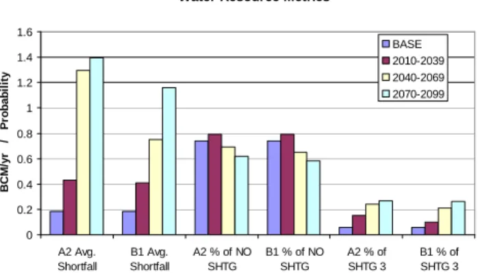
Water Resource Metrics 0 0.2 0.4 0.6 0.8 1 1.2 1.4 1.6 A2 Avg. Shortfall B1 Avg. Shortfall A2 % of NO SHTG B1 % of NO SHTG A2 % of SHTG 3 B1 % of SHTG 3 B C M /y r / P ro b a b il it y BASE 2010-2039 2040-2069 2070-2099
Fig. 9. Average shortfall per year, percentage of years with no
short-fall and percentage of years with a level 3 shortage for the base run and SRES A2 and B1 scenarios.
reservoir storage of 120% of base is a function of very high initial reservoir levels (>56 BCM) and very high early period streamflow and low late period streamflow. Another outlier in Fig. 8 is the B1, period 1 simulation (MRI) in which 110% of base streamflow drives a storage reduction. This is a re-sult of MRI having very low streamflow prior to 2010 and a result, total initial reservoir storage of only 17 BCM.
Although these results seem inconsistent with the greater storage reductions predicted by Christensen et al. (2004), they are within the same range of sensitivity. Christensen et al. (2004) predicted streamflow reductions at the high end of those simulated for individual ensemble members for this study, and as can be seen in Fig. 8, storage reductions in these ensemble members match those of the 2004 study.
3.5.2 Delivery compliance
Water deliveries are dependent on the storage in Lake Mead; level one shortages are imposed (see Sect. 2.3 for amounts and to which users) when Lake Mead drops below an ele-vation of 327.66 m, level two shortages are imposed at an elevation of 320.04 m, and level three at 312.42 m. If need be, deliveries are decreased further to ensure that the eleva-tion of Lake Mead does not drop below the SNWA’s intake at 304.80 m elevation.
Figure 9 shows the average shortage per year, the percent-age of years with no shortpercent-ages, and the percentpercent-age of years with level three shortages for the 1950–1999 “base” run and for the SRES A2 and B1 ensemble averages for periods 1–3. The base run has delivery shortages in 26% of years. In real-ity, there have not yet been shortages, but they are simulated in the base run here because we force CRRM with 1950– 1999 streamflow and year 2000 demands. Shortages are sim-ulated in the base run between the late 50s and mid 70s, while in real operations upper basin demands were lower and there were no shortages. The A2 and B1 scenarios both have short-ages in 21 (A2; 1, 41, B1; 4, 26)% of years in period 1, 31
(0, 80) and 35 (0, 63)% of years in period 2, and 38 (6, 86) and 42 (6, 71)% in period 3.
Level three shortages beginning at 740 MCM/yr are ini-tially imposed when Lake Mead drops below 312.42 m, but are allowed to increase up to the entirety of the Lower Basin and Mexico’s demand to protect a Lake Mead elevation of 304.80 m. The probability of these shortages, along with the average shortage amount (Fig. 9), are not influenced much by the nuances of the reservoir model (initial storage, stream-flow sequence, etc.). They are also likely to have consid-erable socio-economic effect within the basin. Level three shortages are imposed in the base run in 5% of years, and in 11 (0, 30) and 10 (0, 15)% in period one, 24 (0, 45) and 27 (0, 45)% in period two, and 27 (4, 27) and 26 (0, 33)% in period three for the SRES A2 and B1 ensemble averages, respectively.
The shortfall per year (BCM/yr) is derived by dividing the total shortfall in each period by the number of years in which any shortage delivery is imposed. It is a somewhat redun-dant metric because it is related to the number of level three shortages, however it is important to differentiate between long modest shortfalls and short intense ones. The average shortage in the base run was 0.73 BCM, and 2.1 (0.6, 2.2) and 2.0 (0.6, 2.4) BCM/yr in period one for the A2 and B1 scenario, respectively. Average shortfalls in period two were 4.2 (0, 3.5) and 2.1 (0, 2.4) BCM/yr, and 3.7 (0.6, 3.9) and 2.8 (0.7, 3.8) BCM in period three for A2 and B1, respec-tively. Although there seems to be a lack of correlation be-tween streamflow and average shortage (e.g. SRES A2, pe-riod 2 has greater streamflow than B2 pepe-riod 3, yet higher av-erage shortage), this is entirely an artifact of averaging across ensembles. Tables A.3 and A.4 summarize individual GCM run results.
3.5.3 Hydropower generation
Hydropower generation is a function of head (height of water surface above tailwater elevation) and discharge (volume per unit time) passing through a turbine. Because of the sequenc-ing of the base run streamflow and its bias towards lower storage (i.e. head) for a given inflow, it generates less hy-dropower than the period one A2 and B1 average (Fig. 10). The average energy generated in the base run is 8480 GW-h/yr, while in period one the A2 scenario average generates 8600 (10 100, 6470) GW-h/yr, and in the B2 scenario av-erage 8530 (9670, 8220) GW-h/yr. In period two, the A2 average is 7630 (10 800, 4470), and the B1 average is 7560 (10 330, 4650) GW-h/yr, while in period three A2 is 6900 (8960, 4560) and B1 is 7130 (8840, 4670) GW-h/yr. The re-duction of hydropower prore-duction from period 1 to period 3 is 20% in the A2 scenario and 16% in the B1 scenario, both of which are about twice the corresponding streamflow reduction percentages.
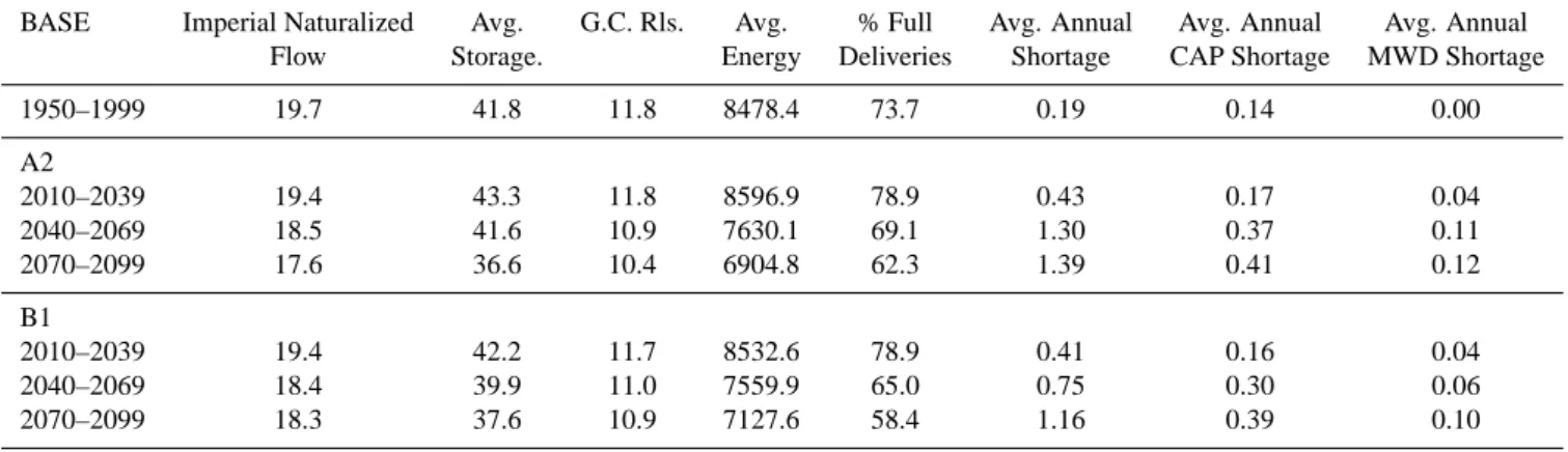
Table 4. Streamflow at Imperial Dam, AZ (BCM/yr), average January 1 total basin storage (BCM), release from Glen Canyon Dam
(BCM/yr), annual energy production (GW-h/yr), percentage of years with no delivery shortages, average annual delivery shortage (BCM/yr), average annual CAP delivery shortage (BCM/yr), and annual average MWD delivery shortage (BCM/yr).
BASE Imperial Naturalized Avg. G.C. Rls. Avg. % Full Avg. Annual Avg. Annual Avg. Annual
Flow Storage. Energy Deliveries Shortage CAP Shortage MWD Shortage
1950–1999 19.7 41.8 11.8 8478.4 73.7 0.19 0.14 0.00 A2 2010–2039 19.4 43.3 11.8 8596.9 78.9 0.43 0.17 0.04 2040–2069 18.5 41.6 10.9 7630.1 69.1 1.30 0.37 0.11 2070–2099 17.6 36.6 10.4 6904.8 62.3 1.39 0.41 0.12 B1 2010–2039 19.4 42.2 11.7 8532.6 78.9 0.41 0.16 0.04 2040–2069 18.4 39.9 11.0 7559.9 65.0 0.75 0.30 0.06 2070–2099 18.3 37.6 10.9 7127.6 58.4 1.16 0.39 0.10
3.5.4 Glen Canyon Dam and Mexico release
The Colorado River Compact mandates a 10 year moving average release of 10.2 BCM/yr from the Upper Basin to the Lower Basin and an annual release of 1.9 BCM (1.5 MAF) from the United States to Mexico. Figure 10 and Table 4 report the detailed results, but in general releases from Glen Canyon Dam are 1 (A2: +1, −1, B1: +6, −6)% less (both B1 and A2) in period one than in the historical run and 7 (+6, −21) and 8 (+10, −21)% lower in period 2 for B1 and A2, respectively. Period 3 has an 8 (+2, −22)% reduction in Glen Canyon releases in the B1 scenario, and a 12 (−4,
−30)% reduction in A2. Although the compact requires the
10.2 BCM/yr release to be made on a 10 year moving aver-age, current basin operations dictate that this release is made annually. The Glen Canyon release drops below 10.2 BCM in 24% of years in the base run, and 28, 35, and 35% of years for the B1 scenario in periods 1–3, respectfully. The Glen Canyon release drops below 10.2 BCM/yr in 28, 34, and 44% of years in the A2 scenario for periods 1–3, respectfully.
Mexico is allocated 17% of the level one through three shortage amount, so the amount of years in which the Lower Basin delivery to Mexico drops below 1.9 BCM is essentially the same as the percentage of years in which any shortages are imposed (see Sect. 3.5.2). The average delivery to Mex-ico in the base run is 1.8 BCM/yr, while the B1 scenario av-erage annual deliveries drop to 1.78 (1.75, 1.83), 1.72 (1.65, 1.81), 1.65 (1.40, 1.81) BCM for periods 1–3 respectfully. In periods 1–3 of the A2 scenario, average annual deliveries are 1.78 (1.72, 1.89), 1.63 (1.45, 1.87), 1.62 (1.48, 1.80) BCM, respectfully.
Water Resource Metrics
0 2 4 6 8 10 12 14
A2 HYDRO PWR B1 HYDRO PWR A2 GC REL B1 GC REL A2 MEX REL B1 MEX REL
K G W -h r/ y r / B C M /y r Base 2010-2039 2040-2069 2070-2099
Fig. 10. Average hydropower production (KGW-h/yr), average
an-nual release from Glen Canyon Dam (BCM/yr), and average anan-nual release to Mexico (BCM/yr) for the base run and period 1–3 for the SRES A2 and B1 scenarios.
4 Conclusions
As compared with earlier studies of climate sensitivity of CRB water resources to climate change, we have assessed in detail the implications of eleven downscaled IPCC climate model scenarios and two emissions scenarios, each one of which constitutes an ensemble member. Therefore, we are able to evaluate the range of possible consequences as repre-sented by the different models and emissions scenarios, in-cluding “consensus” (mean) results, and measures of vari-ability, in particular, the lower and upper quartiles. In this respect, this study is the most comprehensive to date of the implications of climate change on the Colorado River reser-voir system.
As in essentially all previous studies, average annual tem-peratures over the CRB increase with time, not only in the ensemble mean, but for all individual climate models and time period. With the exception of the early part of the cen-tury when the A2 and B1 emission scenarios are similar and
natural variability can dominate the emissions signal, tem-peratures are greater for the A2 emission scenario than for B1. Average temperature increases for the period 2070–2099 are 2.75◦C (with a range of +/−1.0◦C) for the B1 scenario
and 4.35◦C (+/−1.5◦C) for the A2 scenario.
While all models agree with respect to the direction of temperature changes, there is considerable variability in the magnitude, direction, and seasonality of projected precipi-tation changes. Averaged over models, annual precipiprecipi-tation changes are quite small – a maximum change (decrease) of 2% for period 2 and 3 for the A2 emissions scenario. The variability across models is, in general, much larger than the annual change. More apparent in the ensemble means are shifts in seasonality of precipitation, which, in the ensemble mean, all show a shift towards more winter and less summer precipitation. Because winter precipitation (especially in the upper basin) contributes proportionately more to runoff than does summer precipitation, these shifts tend to counteract re-ductions in annual runoff that otherwise would result from increased temperatures (hence evapotranspiration) This shift toward winter precipitation is prevalent in the ensemble av-erage for all periods and scenarios and is most pronounced for the basin upstream of Lees Ferry. Nonetheless, while this shift reduces the effect of increased temperatures on runoff, it does not reverse them, and in the ensemble mean streamflow decreases for all periods on both emissions scenarios.
Runoff changes are driven by combined effects of tem-perature and precipitation changes and their seasonality. In the ensemble means, runoff declines for all periods and both emissions scenarios, with the greatest changes occurring in period 3 for the A2 emissions scenario. Most (ensemble mean) changes in annual streamflow at Lees Ferry are in the single digit percentages, ranging up to an 11% streamflow reduction for emissions scenario A2 in period 3. The range of changes across ensembles is quite large, however, for in-stance for emissions scenario A2 in period 3 the range is from
−37 to +11%.
The runoff changes we project are considerably less in the ensemble mean than those inferred for the U.S. Southwest in recent studies by Milly et al. (2005) and Seager et al. (2007). Both these studies use IPCC AR4 ensembles, but are based on runoff (or equivalently, atmospheric convergence) simu-lated directly by GCMs over the region. Aside from differ-ences in the specific locale and the GCMs analyzed (which we do not believe account for the bulk of the differences), the smaller runoff sensitivity to climate changes in this study appears to be traceable to the sensitivity of annual evapo-transpiration to seasonal shifts in runoff and evapotranspira-tion timing. In the ensemble mean, we find that projected annual precipitation changes are small, hence runoff reduc-tions should be attributable mostly to differences in evapo-transpiration. Our hydrological model operates at consider-ably higher spatial resolution than the native resolution of the GCMs, hence is better able to resolve the interactions of elevation with seasonally varying evaporative demands. In
short, there is a negative feedback between increased temper-ature, which shifts snowmelt timing, and hence soil moisture, earlier in the year, when evaporative demands are lower, and in turn reduces runoff and ET sensitivity to increased tem-perature. This effect is especially important over the rela-tively small high elevation headwaters area where most of the CRB’s runoff is generated. The GCMs are not able to resolve this effect well as their coarse spatial resolution precludes their representing high elevation headwater areas. However, understanding of the nature of this feedback, and the extent to which it explains differences in sensitivities between this study, and Milly et al. (2005) and Seager et al. (2007) is a topic of both scientific and practical importance that deserves further attention.
Due to the fragile equilibrium of the managed water re-sources of the system, any decrease in streamflow results in storage and hydropower decreases, compact violations, and delivery reductions. There are many nonlinearities in the reservoir system response to streamflow, which in general are reflected in amplifications of the range of responses across the ensemble members (models). In general, changes in to-tal basin storage amplify changes in streamflow, and very roughly, for modest (e.g. single digit) percentage changes in streamflow, the storage changes (also expressed as percent-ages) are about double.
Although our results show somewhat smaller (ensemble mean) reductions in runoff over the next century than in pre-vious studies (Christensen et al, 2004 in particular), the reser-voir system simulations show nonetheless that supply may be reduced below current demand which in turn will cause con-siderable degradation of system performance. Reductions in total basin storage, Compact mandated deliveries, and hy-dropower production increase throughout the century, and are larger in the A2 than the B1 scenario. Although not ana-lyzed explicitly in this paper (see Christensen (2004) for de-tails) increasing Upper Basin demands towards their full en-titlement will further exacerbate these reservoir performance issues.
Due to the already large storage to inflow ratio of the CRB, neither increases in reservoir capacity nor changes in operat-ing policies are likely to mitigate these stresses substantially. Clearly depletions (including reservoir evaporation) cannot exceed supply in the long term. Furthermore, due to the high coefficient of variation of annual streamflows in the CRB, and notwithstanding the system’s large reservoir storage, the system is likely to become more susceptible to long term sustained droughts if the excess of supply over demand is reduced, as is suggested by the ensemble means in our study.
Appendix A
Detailed downscaled GCM results and derived (VIC hydrologic model) variables
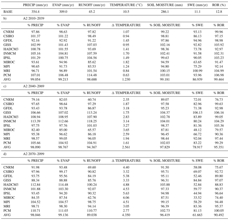
Table A1. a) 1950–1999 “base” mean annual precipitation, evaporation, runoff, temperature, soil moisture, SWE, and runoff ratio in mm/yr
and mm; b), c), d) Period 1–3 SRES A2 mean annual precipitation, evaporation, runoff, temperature, soil moisture, snow water equivalent (SWE), and runoff ratio (ROR) (all as percentages of 1950–1999 base, except temperature which is in◦C change relative to base).
a) 1950–1999
PRECIP (mm/yr) EVAP (mm/yr) RUNOFF (mm/yr) TEMPERATURE (◦C) SOIL MOISTURE (mm) SWE (mm/yr) ROR (%)
BASE 354.4 309.0 45.2 10.5 286.1 11.1 12.8 b) A2 2010–2039
% PRECIP % EVAP % RUNOFF 1 TEMPERATURE % SOIL MOISTURE % SWE % ROR CNRM 97.86 98.63 97.82 1.07 99.22 93.13 99.96 CSIRO 101.37 101.22 98.49 0.94 98.81 86.13 97.15 GFDL 92.16 92.92 91.22 1.45 97.86 94.96 98.98 GISS 102.99 101.43 107.03 0.95 102.16 92.82 103.92 HADCM3 100.78 101.55 93.69 1.41 98.36 73.78 92.97 INMCM 105.16 104.81 107.59 1.70 102.41 91.58 102.31 IPSL 101.29 100.75 104.56 1.49 99.63 90.05 103.23 MIROC 93.61 94.96 85.62 1.82 94.59 63.65 91.47 MPI 90.65 91.73 83.53 1.24 94.80 75.29 92.14 MRI 96.71 96.89 101.54 0.84 100.15 100.99 104.99 PCM 107.01 106.48 114.48 0.63 103.01 93.96 106.98 AVG 99.054 99.213 98.688 1.230 99.181 86.939 99.464 c) A2 2040–2069
% PRECIP % EVAP % RUNOFF 1 TEMPERATURE % SOIL MOISTURE % SWE % ROR CNRM 79.16 82.03 60.74 2.35 89.07 72.01 76.73 CSIRO 97.65 98.64 97.29 1.87 97.58 82.96 99.63 GFDL 93.43 93.78 86.87 3.18 95.23 71.38 92.98 GISS 106.66 107.02 113.24 1.75 104.37 106.13 106.16 HADCM3 108.94 108.95 107.90 2.83 102.78 83.89 99.05 INMCM 113.39 112.66 118.25 3.14 104.01 80.24 104.29 IPSL 97.75 97.76 101.03 3.27 98.37 81.36 103.36 MIROC 82.40 85.00 65.57 3.65 87.81 48.12 79.57 MPI 95.38 96.62 86.18 2.59 96.45 66.72 90.36 MRI 98.57 99.05 96.05 1.94 98.44 92.04 97.44 PCM 105.66 104.92 104.91 1.61 102.03 83.22 99.29 AVG 98.090 98.767 94.367 2.561 97.829 78.917 95.351 d) A2 2070–2099
% PRECIP % EVAP % RUNOFF 1 TEMPERATURE % SOIL MOISTURE % SWE % ROR CNRM 91.98 93.48 69.60 4.40 91.50 58.08 75.67 CSIRO 97.96 99.17 90.82 3.32 95.71 69.07 92.72 GFDL 93.75 95.56 84.19 5.38 95.11 52.46 89.80 GISS 88.34 88.88 85.76 3.33 96.31 84.84 97.07 HADCM3 112.84 114.48 100.24 4.88 103.88 52.84 88.83 INMCM 101.88 103.30 92.07 4.53 97.33 59.77 90.37 IPSL 93.45 94.20 90.32 5.63 94.98 44.94 96.64 MIROC 84.35 87.54 62.76 6.06 87.51 33.52 74.40 MPI 104.52 104.57 98.75 4.51 99.15 58.29 94.48 MRI 98.71 98.30 94.14 3.05 96.39 83.36 95.37 PCM 110.71 111.03 110.77 2.77 102.73 81.13 100.05 AVG 98.046 99.136 89.038 4.350 96.419 61.663 90.492
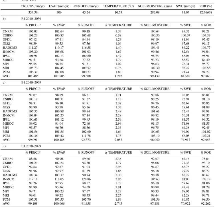
Table A2. a) 1950–1999 (base) mean annual precipitation, evaporation, runoff, temperature, soil moisture, snow water equivalent (SWE),
and runoff ratio (ROR) in mm/yr and mm (◦C for temperature). b, c, d) Period 1–3 SRES B1 precipitation, evaporation, runoff, temperature, soil moisture, SWE, and runoff ratio as percentage of 1950–1999 base.
a) 1950–1999
PRECIP (mm/yr) EVAP (mm/yr) RUNOFF (mm/yr) TEMPERATURE (◦C) SOIL MOISTURE (mm) SWE (mm/yr) ROR (%)
354.36 309 45.24 10.53 286.08 11.07 12.76668 b) B1 2010–2039
% PRECIP % EVAP % RUNOFF 1 TEMPERATURE % SOIL MOISTURE % SWE % ROR CNRM 102.03 102.64 99.18 1.33 100.64 89.32 97.21 CSIRO 101.23 100.83 105.68 0.58 100.30 100.07 104.39 GFDL 97.12 97.41 94.64 1.26 98.19 81.94 97.45 GISS 98.39 99.53 97.56 1.04 99.97 97.68 99.15 HADCM3 111.27 110.17 116.58 1.40 104.41 86.22 104.77 INMCM 105.20 105.68 101.03 1.67 99.46 82.56 96.04 IPSL 101.91 102.14 100.80 1.42 98.75 88.06 98.91 MIROC 91.51 93.68 77.32 1.79 93.23 58.59 84.49 MPI 95.55 96.25 91.51 1.02 96.63 76.31 95.77 MRI 105.73 104.45 109.52 0.76 102.30 98.27 103.58 PCM 106.39 107.08 100.77 1.83 99.94 71.44 94.72 AVG 101.485 101.805 99.508 1.282 99.439 84.588 97.863 c) B1 2040–2069
% PRECIP % EVAP % RUNOFF 1 TEMPERATURE % SOIL MOISTURE % SWE % ROR CNRM 97.07 98.89 86.21 1.71 97.86 78.05 88.81 CSIRO 100.19 101.31 91.27 1.13 98.25 72.94 91.10 GFDL 94.31 96.10 81.91 2.37 94.76 62.67 86.85 GISS 92.90 93.78 85.36 1.33 96.45 79.61 91.89 HADCM3 105.35 106.88 98.94 2.48 101.61 72.44 93.91 INMCM 104.04 105.25 97.14 2.28 99.82 70.31 93.37 IPSL 100.63 101.12 99.95 2.59 98.19 81.55 99.32 MIROC 89.02 91.04 72.60 2.99 91.13 51.98 81.55 MPI 95.57 96.70 88.36 2.33 96.75 69.38 92.45 MRI 101.56 101.55 102.60 1.64 100.63 99.09 101.02 PCM 109.36 109.42 111.78 1.73 103.10 86.08 102.21 AVG 99.091 100.185 92.373 2.052 98.050 74.917 92.953 d) B1 2070–2099
% PRECIP % EVAP % RUNOFF 1 TEMPERATURE % SOIL MOISTURE % SWE % ROR CNRM 88.58 90.90 69.66 2.35 92.67 67.16 78.64 CSIRO 101.29 102.24 94.30 1.77 98.06 77.33 93.10 GFDL 92.64 92.87 91.03 2.96 94.67 68.78 98.27 GISS 91.96 92.97 81.59 1.85 96.18 79.27 88.72 HADCM3 102.34 103.37 90.74 3.30 98.38 68.29 88.67 INMCM 119.18 118.05 128.86 2.96 105.63 81.00 108.12 IPSL 97.26 97.95 88.57 3.73 96.10 59.69 91.06 MIROC 91.90 95.36 74.69 3.91 90.98 47.47 81.28 MPI 98.71 100.23 87.67 3.23 96.33 68.02 88.81 MRI 99.01 99.22 98.73 2.25 98.44 82.28 99.71 PCM 107.31 107.55 105.70 1.89 101.56 80.85 98.50 AVG 99.108 100.066 91.958 2.745 97.181 70.922 92.262
Table A3. Average annual naturalized flow at Imperial Dam (BCM/yr), average total simulated basin storage (BCM), annual release from
Glen Canyon Dam (BCM/yr), average annual energy production (GW-h/yr), percent of years with full deliveries (%), average annual delivery shortfall (BCM/yr), average annual CAP shortfall (BCM/yr), and average annual MWD shortfall (BCM/yr) for a) 1950–1999 base run and b), c), d) for SRES A2 scenario for Periods 1–3.
a) 1950–1999 Imperial Naturalized Flow (BCM/yr) Avg. Storage. (BCM) G.C. Rls. (BCM/yr) Avg. Energy (GW-h/yr) % Full Deliveries (%) Avg. Annual Shortage (BCM/yr)
Avg. Annual CAP Shortage (BCM/yr) Avg. Annual MWD Shortage (BCM/yr) 19.7 41.8 11.8 8478 73.7 0.19 0.14 0 b) A2 2010–2039 Imperial Naturalized Flow (BCM/yr) Avg. Storage (BCM) G.C. Rls. (BCM/yr) Avg. Energy (GW-h/yr) % Full Deliveries (%) Avg. Annual Shortage (BCM/yr)
Avg. Annual CAP Shortage (BCM/yr) Avg. Annual MWD Shortage (BCM/yr) cnrm 19.2 48.7 12.0 9812 99.2 0.00 0.00 0.00 cisro 19.3 41.0 11.4 8204 81.7 0.11 0.09 0.00 gfdl 17.9 35.8 10.7 7865 82.5 0.10 0.08 0.00 giss 20.9 49.3 13.0 9909 88.6 0.16 0.08 0.01 hadcm3 17.7 29.8 10.2 5483 41.4 1.36 0.54 0.12 inmcm 21.2 55.5 13.4 10716 95.8 0.02 0.02 0.00 ipsl 20.6 50.5 12.4 9823 99.7 0.00 0.00 0.00 miroc 17.2 33.5 10.2 6468 58.3 1.30 0.42 0.11 mpi 16.4 24.9 9.4 4658 20.3 1.72 0.69 0.15 mri 20.5 51.6 12.5 10139 100.0 0.00 0.00 0.00 pcm 22.3 56.5 14.4 11489 100.0 0.00 0.00 0.00 AVG 19.4 43.4 11.8 8597 78.9 0.43 0.17 0.04 c) A2 2040–2069 Imperial Naturalized Flow (BCM/yr) Avg. Storage (BCM) G.C. Rls. (BCM/yr) Avg. Energy (GW-h/yr) % Full Deliveries (%) Avg. Annual Shortage (BCM/yr)
Avg. Annual CAP Shortage (BCM/yr) Avg. Annual MWD Shortage (BCM/yr) cnrm 11.8 17.3 5.5 1319 0.0 5.95 1.46 0.52 cisro 19.1 51.0 11.6 9503 99.2 0.00 0.00 0.00 gfdl 16.7 25.1 9.3 4467 28.9 1.98 0.67 0.15 giss 22.0 57.7 13.4 10871 99.7 0.00 0.00 0.00 hadcm3 20.5 49.7 11.9 9432 100.0 0.00 0.00 0.00 inmcm 23.1 58.8 14.2 11649 100.0 0.00 0.00 0.00 ipsl 20.6 55.9 13.0 10798 100.0 0.00 0.00 0.00 miroc 13.2 20.4 6.8 2436 12.2 4.85 1.28 0.46 mpi 16.8 27.4 9.9 5465 36.9 1.08 0.48 0.08 mri 19.0 43.5 11.2 8236 82.8 0.38 0.14 0.03 pcm 20.1 51.2 12.0 9754 100.0 0.00 0.00 0.00 AVG 18.5 41.6 10.8 7630 69.1 1.30 0.37 0.11 d) A2 2070–2099 Imperial Naturalized Flow (BCM/yr) Avg. Storage (BCM) G.C. Rls. (BCM/yr) Avg. Energy (GW-h/yr) % Full Deliveries (%) Avg. Annual Shortage (BCM/yr)
Avg. Annual CAP Shortage (BCM/yr) Avg. Annual MWD Shortage (BCM/yr) cnrm 13.5 19.3 6.5 2318 9.7 4.66 1.20 0.42 cisro 18.3 32.1 10.7 6491 60.3 0.82 0.35 0.07 gfdl 16.4 25.4 9.4 4559 28.9 1.76 0.66 0.15 giss 16.9 34.2 10.4 7322 67.8 0.49 0.20 0.03 hadcm3 19.2 46.7 11.4 9041 95.6 0.02 0.02 0.00 inmcm 18.2 43.7 11.1 8529 94.4 0.03 0.03 0.00 ipsl 18.5 41.2 11.0 8105 80.3 0.45 0.15 0.03 miroc 12.6 18.6 6.4 1782 0.0 5.49 1.38 0.48 mpi 19.8 41.5 11.7 7586 61.1 1.50 0.46 0.13 mri 19.1 45.6 11.4 8961 88.1 0.12 0.08 0.01 pcm 21.5 54.1 14.0 11259 98.9 0.01 0.00 0.00 AVG 17.6 36.6 10.4 6905 62.3 1.40 0.41 0.12
Table A4. Average annual naturalized flow at Imperial Dam (BCM/yr), average total simulated basin storage (BCM), annual release from
Glen Canyon Dam (BCM/yr), average annual energy production (GW-h/yr), percent of years with full deliveries (%), average annual delivery shortfall (BCM/yr), average annual CAP shortfall (BCM/yr), and average annual MWD shortfall (BCM/yr) for a) 1950–1999 base run and b), c), d) for SRES B1 scenario for Periods 1–3.
a) 1950–1999 Imperial Naturalized Flow (BCM/yr) Avg. Storage (BCM) G.C. Rls. (BCM/yr) Avg. Energy (GW-h/yr) % Full Deliveries (%) Avg. Annual Shortage (BCM/yr)
Avg. Annual CAP Shortage (BCM/yr) Avg. Annual MWD Shortage (BCM/yr) 19.7 41.8 11.8 8478 73.7 0.19 0.14 0 b) B1 2010–2039 Imperial Naturalized Flow (BCM/yr) Avg. Storage (BCM) G.C. Rls. (BCM/yr) Avg. Energy (GW-h/yr) % Full Deliveries (%) Avg. Annual Shortage (BCM/yr)
Avg. Annual CAP Shortage (BCM/yr) Avg. Annual MWD Shortage (BCM/yr) cnrm 19.7 39.5 11.6 8215 89.4 0.22 0.10 0.02 cisro 20.5 46.6 12.7 8989 69.4 0.35 0.19 0.02 gfdl 18.3 36.2 11.1 7979 81.7 0.10 0.08 0.00 giss 18.9 48.0 12.1 9670 95.8 0.02 0.02 0.00 hadcm3 21.5 55.9 13.2 10791 100.0 0.00 0.00 0.00 inmcm 19.7 43.0 11.6 8159 73.1 0.39 0.18 0.02 ipsl 20.0 44.9 12.5 9484 89.2 0.06 0.05 0.00 miroc 15.4 24.2 9.0 4290 20.6 2.30 0.76 0.20 mpi 17.9 34.2 10.8 7691 74.7 0.14 0.11 0.00 mri 21.2 41.0 12.6 8771 74.4 0.92 0.28 0.08 pcm 20.0 50.7 12.2 9820 100.0 0.00 0.00 0.00 AVG 19.4 42.2 11.7 8533 78.9 0.41 0.16 0.03 c) B1 2040–2069 Imperial Naturalized Flow (BCM/yr) Avg. Storage (BCM) G.C. Rls. (BCM/yr) Avg. Energy (GW-h/yr) % Full Deliveries (%) Avg. Annual Shortage (BCM/yr)
Avg. Annual CAP Shortage (BCM/yr) Avg. Annual MWD Shortage (BCM/yr) cnrm 17.4 38.2 10.3 7565 78.1 0.33 0.15 0.02 cisro 18.2 42.1 10.9 8589 97.8 0.01 0.01 0.00 gfdl 16.5 24.4 9.9 4646 14.7 1.38 0.63 0.11 giss 16.9 29.3 9.9 5607 42.2 1.47 0.52 0.12 hadcm3 19.1 47.9 11.3 9085 91.1 0.05 0.04 0.00 inmcm 18.5 39.4 10.7 7430 69.4 0.36 0.20 0.02 ipsl 20.2 55.1 12.6 10330 100.0 0.00 0.00 0.00 miroc 14.8 20.7 8.4 2902 2.2 3.08 1.07 0.30 mpi 16.8 23.7 9.4 4335 19.7 1.54 0.66 0.13 mri 20.4 58.0 12.6 10580 100.0 0.00 0.00 0.00 pcm 22.7 59.8 14.8 12091 100.0 0.00 0.00 0.00 AVG 18.3 39.9 11.0 7560 65.0 0.75 0.30 0.06 d) B1 2070—2099 Imperial Naturalized Flow (BCM/yr) Avg. Storage (BCM) G.C. Rls. (BCM/yr) Avg. Energy (GW-h/yr) % Full Deliveries (%) Avg. Annual Shortage (BCM/yr)
Avg. Annual CAP Shortage (BCM/yr) Avg. Annual MWD Shortage (BCM/yr) cnrm 13.4 18.4 6.4 1877 0.0 4.70 1.28 0.43 cisro 18.9 39.8 11.3 7947 75.0 0.15 0.12 0.00 gfdl 18.4 34.7 11.1 6911 52.5 0.78 0.35 0.06 giss 16.4 23.3 9.2 4074 13.9 2.15 0.81 0.19 hadcm3 18.1 39.7 10.8 7084 65.8 1.01 0.35 0.08 inmcm 24.3 56.5 14.8 11978 100.0 0.00 0.00 0.00 ipsl 17.6 50.1 10.5 8813 94.2 0.23 0.06 0.02 miroc 15.3 21.8 8.7 3464 8.9 2.99 0.96 0.26 mpi 17.7 29.4 10.7 6533 50.3 0.65 0.32 0.04 mri 19.7 42.3 12.1 8869 81.7 0.12 0.09 0.00 pcm 21.0 57.5 13.2 10853 100.0 0.00 0.00 0.00 AVG 18.3 37.6 10.8 7128 58.4 1.16 0.40 0.10