Design of a power-scalable digital least-means-square adaptive filter

Design of A Power-Scalable Digital

Least-Means-Square Adaptive Filter

by

Chee We Ng

Submitted to the Department of Electrical Engineering and Computer

Science

in partial fulfillment of the requirements for the degree of

Masters of Engineering in Electrical Engineering and Computer

Science

at the

MASSACHUSETTS INSTITUTE OF

February

2001

UL

112001

@

_{Chee We Ng, MMI. All rights reserved.}

LIBRARIES--The author hereby grants to MIT permission to reproduce and

distribute publicly paper and electronic copies of this thesis documentBARKER

in whole or in part.

A uthor ...

Department of Electrical Engineering and CompiYter Science

December, 2000

Certified by...

Anantha Chandrakasan

Associate Professor

--

egis Supeyisor

Arthu C. Smith

Chairman, Department Committee on Graduate Students

Design of A Power-Scalable Digital Least-Means-Square

Adaptive Filter

by

Chee We Ng

Submitted to the Department of Electrical Engineering and Computer Science on December, 2000, in partial fulfillment of the

requirements for the degree of

Masters of Engineering in Electrical Engineering and Computer Science

Abstract

This thesis describes the design of power-scalable digital adaptive equalizer for pulse or quadrature amplitude modulation communication systems, using synthesis and place-and-route tools. DSP based modem applications such as gigabit Ethernet transceivers require channel equalization. Because of the high rate and computation complexity involved, adaptive equalization filters consume a lot of power. Currently, equalization is typically hardwired instead of using a digital signal processor. Yet, there is a need for the equalization filters to be scalable to different channel and bit rate requirements. Synthesis and place-and-route tools enables the designer to focus on higher-level aspects of the design instead of at the transistor level. In this thesis, we have used adaptive tap length and precision techniques to design a digital adaptive equalizer whose power consumption is scalable to the precision requirements.

Thesis Supervisor: Anantha Chandrakasan Title: Associate Professor

Acknowledgments

To the professors, recitation instructors, and teaching assistants of the 6.00x, 6.01x introductory Electrical Engineering and Computer Science classes, who taught me to focus on understanding the fundamentals and gave me the confidence to always seek out the right answer to questions: Prof. Jeffrey Lang, Prof. Dimitri Antoniadis, Prof. Alan Willsky, Prof. Clifton Fonstad, Prof. George Verghese, and Andrew Kim.

To Prof. Stephen Senturia, who convinced me doing well in one class is better than taking seven classes each semester.

To the upperclassmen I knew as a freshmen, who showed me how to get the most out of MIT.

To the friends, who kept me inspired with their warmth and graciousness. To our research group, for the help and company.

To particular individuals who helped me tremendously in my thesis, without who my thesis may not have been completed: Don Hitko and Jim Goodman.

To Prof. Anantha Chandrakasan, for giving me the opportunity to work on this thesis. I learnt lifelong lessons in perseverance and decisiveness.

To my parents and siblings. Thank you all.

Contents

1 Introduction and Objective 12

1.1 M otivation . . . . 12

1.1.1 Low Power Digital CMOS Methodologies . . . . 12

1.1.2 A Power-Scalable Least Mean Squares Adaptive Filter . . . . 13

1.2 Thesis Overview . . . . 15

2 Overview of Least Mean Squares Adaptive Filters 16 2.1 The Equalizer Problem and the Least Mean Squares Stochastic Gra-dient Algorithm . . . . 16

2.1.1 Fractionally-spaced Decision Feedback Equalizers . . . . 19

2.1.2 Convergence and Stability . . . . 21

2.1.3 Tap Precision . . . . 22

2.1.4 Length of Equalizer . . . . 22

2.1.5 Training Sequences and Blind Equalization . . . . 22

2.2 Previous Work on Low Power Adaptive Decision Feedback Equalizers 23 3 Scalable Adaptive Filter: Signal Processing Issues 27 3.1 Design Overview . . . . 27

3.1.1 Design Objective . . . . 27

3.1.2 Design Approach . . . . 27

3.2 Fixed Point MATLAB Model . . . . 28

3.2.1 A rchitecture . . . . 28

3.2.3 Dynamic Range and Precision:

Input, Output, Taps, and Intermediate Results . . . . 30

3.2.4 Rounding off Intermediate Results . . . . 32

3.2.5 Simulation Results . . . . 32

3.3 Performance of LMS Adaptive Filter . . . . 34

3.3.1 Convergence Issues . . . . 34

3.3.2 Steady State Output Error, Filter Length and Tap Precision . 35 3.4 Power Consumption of the Baseline LMS Adaptive Filter . . . . 39

3.4.1 Power Dissipation in a Signed Multiplier . . . . 40

3.5 Power-Scalable Adaptive Filter Architecture . . . . 43

4 Scalable Adaptive Filter: Implementation and Results 46 4.1 O verview . . . . 46

4.1.1 Behavioral Description, Simulation, and Synthesis . . . . 47

4.1.2 Preliminary Verification and Power Estimation . . . . 48

4.1.3 Place and Route, Incorporating Front-end Cell Views, and Ex-traction to SPICE . . . . 48

4.1.4 Design Verification and Power Estimation . . . . 48

4.2 Im plem entation . . . . 49

4.2.1 Implementing Adjustable Length . . . . 50

4.2.2 Implementing Adjustable Tap-precision . . . . 50

4.2.3 Control Logic . . . . 51

4.2.4 VHDL Description of Filter Structure . . . . 55

4.3 R esults . . . . 56

4.3.1 Synthesis and Layout . . . . 56

5 Conclusions and Future Work 59 A Design Documentation: Scalable Fifteen Tap Adaptive Filter 60 A .1 Top Level . . . . 60

A.2 Clock-gating . . . . 63

A.3 Five-tap buiilding block . . . . 64

B Tutorial: Using the Synthesis and Place-and-Route Design Flow 69 B.1 Basic Synthesis and Layout: An Example . . . . 69

B.1.1 Synthesis . . . . 69

B.1.2 Place-and-Route . . . . 70

B.2 Extraction . . . . 79

B.3 Running Powermill . . . . 81

C Tutorial: Setting Up the Synthesis and Place-and-Route Design Flow 87 C.1 Data files for CAD Tools . . . . 88

C.2 Setting Up Design Analyzer . . . . 88

C.3 Setting Up Cadence Silicon Ensemble . . . . 89

C.4 Setting up Design Framework . . . . 89

List of Figures

1-1 Typical PAM/QAM communications system. ... 13

1-2 Decision-feedback equalizer. ... ... 14

2-1 Channel impulse response and data sampling points, illustrating Inter-symbol interference. [Reproduced from [2]] . . . . 17

2-2 Least Mean Square Adaptive Filter. . . . . 19

2-3 Decision-feedback equalizer. [Reproduced from [21] . . . . 20

2-4 Spectrum of baseband signal input to a FSE and a TSE. . . . . 20

2-5 Two Hybrid Forms of an FIR Filter. [Reproduced from [1]] . . . . 23

2-6 An FIR Filter using time-multiplexed multipliers. [Reproduced from [1]] 24 2-7 Measured power per multiplier in FIR filter employing time-multiplexed Booth recoded multipliers. [Reproduced from [1]] . . . . 24

2-8 Programmable Gain. [Reproduced from [1]] . . . . 25

2-9 Power reduction techniques. [Reproduced from [1]] . . . . 25

3-1 Basic six tap LMS adaptive filter. . . . . 28

3-2 Basic six tap LMS adaptive filter in MATLAB Simulink. . . . . 29

3-3 Simulation of the basic six tap LMS adaptive filter. . . . . 33

3-4 Performance comparison of a infinite precision versus finite precision filter. . . . . 35 3-5 Performance of filter with varying tap length, tap precision and adder

precision, using round-down arithmetic, for ISI over two time samples. 36 3-6 Performance of filter with varying tap length, tap precision and adder

3-7 Performance of filter with varying tap length, tap precision and adder

precision, using round-to-zero arithmetic, for ISI over two time samples.

3-8 Six tap Baseline filter. . . . .

3-9 Power consumption of signed-multipliers of various bit-length given the

sam e 6-bit input. . . . .

3-10 Comparing using large multipliers for small inputs when inputs are

placed at the least significant and most significant bits. . . . .

3-11 Block diagram of a power-scalable LMS adaptive filter. . . . .

4-1 Overall architecture. . . . . 4-2 Turning off a block by gating the clocks, reseting the registers, and

latching the input to multipliers. . . . .

4-3 Low-precision mode by gating the clock to the lower precision bit reg-isters and using lower precision multipliers.

4-4 4-5 4-6 4-7 4-8

Architecture of control logic. . . . . Behavior of Clock-gating Circuit. . . . . Clock-gating Circuit. . . . .

Layout of Circuit. . . . . Trade-off between power and standard deviation of error at output. .

B-1 Design Analyzer. . . . . B-2 Silicon Ensemble Import LEF Dialog. . . .

B-3 Silicon Ensemble Import Verilog Dialog. B-4 Silicon Ensemble Initialize Floorplan. . . .

B-5 Silicon Ensemble Place IOs. . . . . B-6 Silicon Ensemble Place Cells. . . . . B-7 Silicon Ensemble window after placement.

B-8 Silicon Ensemble Add Filler Cells... B-9 Silicon Ensemble Add Rings. . . . . B-10 Silicon Ensemble window after routing. . . B-11 Silicon Ensemble Export GDSII. . . . .

38 40 41 43 45 49 50 . . . . 51 52 54 55 57 58 . . . . 7 0 . . . . 7 1 . . . . 7 2 . . . . 7 3 . . . . 7 4 . . . . 7 4 . . . . 7 5 . . . . 7 6 . . . . 7 7 . . . . 7 8 78

B-12 Design Framework Stream In. Click "User-Defined Data" on the left dialog for the right dialog to appear. . . . . 79

B-13 Design Design Framework Virtuoso Layout. . . . . 80

List of Tables

3.1 Representation of input, taps, intermediate results and outputs, and the normalization needed before the next operator. The representation

p.q means that the integer portion has p bits and the fractional portion

has q bits, and the representation s#r represents that the variable has

s bits, and the actual value the s-bit integer multiplied by 2- . . . 31

3.2 Examples of channel responses . . . . 35 3.3 Critical path delays. . . . . 40 3.4 Breakdown of power dissipation. Total power consumption is 6.16 mW. 41

3.5 Breakdown of capacitances. . . . . 41

3.6 Comparison of power consumption of a 10 by 11 bit multiplier versus a 10 by 16 bit multiplier given the same set of 10 bit and 11 bit inputs, at a clock frequency of 100MHz. . . . . 42

3.7 Representation of input, taps, intermediate results and outputs, and the normalization needed before the next operator. . . . . 45

4.1 CAD Tools in a digital design flow . . . . 46

4.2 A digital design flow . . . . 47

4.3 _{Control signals for each sub-block. When the sub-block is turned off,} all clock signals are gated, and resets are set high. . . . . 49 4.4 Critical path delays. . . . . 56

4.5 Breakdown of power dissipation (mW) for scalable 15 tap filter. . . . 56

4.6 Breakdown of capacitances(pF) for scalable 15 tap filter. . . . . 57

Chapter 1

Introduction and Objective

1.1

Motivation

In recent years, power consumption in digital CMOS has become an increasingly important issue. In portable applications, a major factor in the weight and size of the devices is the amount of batteries, which is directly influenced by the power dissipated

by the electronic circuits. For non-portable devices, cooling issues associated with the

power dissipation has caused significant interest in power reduction.

1.1.1

Low Power Digital CMOS Methodologies

Several general low-power techniques for digital CMOS have been developed [5, 6,

15, 24, 33, 38, 22]. In [5], power reduction schemes for circuit, logic, architecture

and algorithmic levels were proposed. At the circuit and logic level, these techniques include transistor sizing, reduced-swing logic, logic minimization, and clock-gating to power-down unused logic blocks. At the architecture level, optimization techniques include dynamic voltage scaling and pipelining to maintain throughput, minimizing switching activity by a careful choice of number representation, and balancing sig-nal paths. At the algorithm level, these techniques include reducing the number of operations, and using algorithmic transformations.

explored include the following. In [22] and [24], the idea of having the overall system select, during run time, the number of stages required for a filter was introduced and later demonstrated in [38]. [23] and [28] describe low-power FIR techniques

using algebraic transformations. [33] describes an energy efficient filtering approach using bit-serial multiplier-less distributed arithmetic technique. [7] and [9] describes low-power FIR techniques based on differential coefficients and input, and residue arithmetic respectively.

1.1.2

A Power-Scalable Least Mean Squares Adaptive Filter

In this thesis, the system design of a power-scalable least means square (LMS) adaptive filter is described. LMS adaptive filters are used for channel equaliza-tion in modems and transceivers, which are becoming increasing important. These transceivers require channel equalization because channels tend to disperse a data pulse and cause Inter-Symbol Interference (ISI). Causes of dispersion include reflec-tions from impedance mismatches in coaxial cables, filters in voiceband modems and scattering in radios.

White Gaussian Noise

Transmit Receive Waveform " or "O"

Fliter Filter Sampie&

hR(t) Symbol

Decision Decision

Point

t

Figure 1-1: Typical PAM/QAM communications system.

Figure 1-1 shows the block diagram of a typical Pulse/Quadrature Amplitude Modulation (PAM/QAM) system. At the transmitter, the digital data stream is modulated into band-limited pulse shapes by a pulse shaping filter, shifted to the carrier frequency by a mixer, and sent through the channel. At the receiver, the received signal shifted down to baseband, sampled, passed through a matched filter, and an optimum decision slicer and decoder. PAM and QAM systems can have

adjustable bit rates by varying the number of levels of the pulse height from 2(in anti-podal signaling) to any power of 2. QAM systems pack a higher data rate than PAM systems by modulating data streams on a set of two orthogonal waveforms

-the in-phase and quadrature components. The reader is refered to texts such as [29] and [2] for further explanation of these two communication systems.

Input _{Pk

f k

+ Detector

Output

Figure 1-2: Decision-feedback equalizer.

One of the commonly used equalizer is a decision-feedback equalizer [29], depicted in Figure 1-2. It consists of a forward section and a feedback section. The feed-forward section attempts to remove precursor ISI and the feedback section attempts to remove post-cursor ISI. Both sections use the least-means-square adaptive filter algorithm [16]. Note that the difference between a decision-feedback equalizer for

QAM and PAM is that the input streams for QAM are complex numbers and the

multiplication and addition operations are complex, instead of real numbers.

Because of the high rate and computation complexity involved, adaptive equal-ization filters consumes a lot of power. Currently, equalequal-ization is typically hardwired instead of using a digital signal processor because of the large number of operations required per second. [20] cites a requirement of 1440 million operations per second

for a decision feedback equalizer. Current DSPs are capable of about 500 million operations per second. Yet, there is a need for the equalization filters to be scalable to different channel and bit rate requirements.

1.2

Thesis Overview

In this thesis, we have used an adaptive tap length and precision technique to make the power-consumption of a digital adaptive equalizer scalable to the precision require-ments. Our design is a least-means-square (LMS) adaptive filter that can be used for a PAM communication system. Designing it for PAM simplifies our study to focus on one real stream instead of two real streams, and to have a single real multiplier per tap, as opposed to four in a simple implementation of complex multiplication. The evaluation system is a PAM system with ISI.

We have used synthesis and place-and-route tools for this design because they en-able the designer to focus on higher-level aspects of the design instead of the transistor level.

In the following chapter, I will give an background overview of LMS adaptive filters and some recent implementations in Chapter 2.

In Chapter 3, I will discuss the signal processing issues involved in designing a power-scalable adaptive filter, such as in designing a fixed point MATLAB model and in choosing the precision of intermediate results. We will discuss some simulations to study the power dissipation patterns of a base-line equalizer and of two's complement signed-multipliers, and the performance of the LMS filter as tap precision and length is reduced.

In Chapter 4, we will discuss the actual implementation of a power-scalable LMS filter and our findings.

Chapter 2

Overview of Least Mean Squares

Adaptive Filters

This chapter gives an overview of Least Means Squares (LMS) adaptive filters, and previous work on low-power implementations.

2.1

The Equalizer Problem and the Least Mean

Squares Stochastic Gradient Algorithm

Assuming that the channel frequency response is well-known and fixed in time, the pulse shaping filter and matched filter in a QAM/PAM communication system can be designed so that it satisfies the Nyquist Criterion for no ISI. However in many communications systems, particularly in wireless applications, the channel is time varying. Time-varying dispersion moves the zero crossings which are originally located at the centers of all other symbols. Figure 2-1 shows a channel impulse response and the data sampling points, illustrating ISI for a PAM system. The largest data sample is used as a cursor to recover the original data, and the other samples are considered to be ISI. The samples that come before the cursor are called "precursor ISI" and those that come after are called "post-cursor ISI". The role of the channel equalizer is to perform inverse filtering of the channel impulse response.

MM=4

h 2 _h3

Figure 2-1: Channel impulse response and data sampling points, illustrating Inter-symbol interference. [Reproduced from [2]]

The equalizer [2] works in the following way. For the sake of discussion, consider a Finite Impulse Response (FIR) equalization filter. Denote the filter taps as c

[c[O], c[1], c[2],...c[N - 1]]T and the impulse response matrix H defined as

hij = h[i-j+1] for 1 <i-j+1 < M, (2.1)

0 otherwise.

where M is the length of the sampled impulse response truncated. The ideal equalizer should satisfy the following equation

H - c = d (2.2)

where d is the ideal impulse response, i.e. [..o, 0, 1, 0, 0, .. .]. Note that this set of

equations is over-determined. Therefore, it must be solved approximately, either by zero-forcing or Least Mean Squares (LMS).

The mean square error is given by

E_{1 -ET} 2

= (cTHT _{- dT)} .(Hc - d)

cTHTHc- dTHc - cTHTd dTd (2.3)

A value of c can be derived analytically to minimize the mean square error by

com-pleting the squares

16 2 = (CT - dTH(HTH)-) - HTH - (c - (HTH)-lHTd) (2.4)

The optimal filter taps is then

Copt = HTHHTd (2.5)

Iterative adaptation to this solution can be achieved by the method of steepest de-scent. The new tap values are calculated from the old values by

c -

d

C C- dc c (2.6)

A is known as the step size. H and d are not observable. However, if continuous data

is used, we note that

HTH = E[YTY] and HTd = E[YTa] (2.7)

where a is the data stream vector (assumed to be memoryless) and Y is the input signal (to the equalizer) matrix defined as

yi,j = y[i - j + 1] (2.8)

Hence for a continuous data stream, the new taps are typically computed according to

Ck+1 = Ck + AEkYk (2.9)

where the subscriptions represent time intervals and Yk is the kth row of Y and is the input signal contents of the FIR at time kT and

= d - Hc (2.10)

is the expected output minus the output of the filter. In a more commonly used notation, this is

(2.11) where cj [k] is the jth tap at time kT. This is known as the LMS stochastic gradient

method. This kind of filter is also known as a linear equalizer. Figure 2-2 shows a block diagram of the filter.

a[k]@ 0

e[k X -ek X e[k X e[k X

delta delta delta delta

y[k] + + *00 +

Figure 2-2: Least Mean Square Adaptive Filter.

The discussion so far is for PAM. For QAM, we treat the data streams as com-plex numbers, where the in-phase stream is represented by the real part and the quadrature-phase is represented by the imaginary part. The derivation remains the same if we replace the transpose operator with the hermitian operator.

2.1.1

Fractionally-spaced Decision Feedback Equalizers

In modern communication systems, one of the commonly used equalizer is a decision-feedback equalizer [29], depicted in Figure 2-3. It consists of a feed-forward section and a feedback section. The feed-forward section attempts to remove precursor ISI and the feedback section attempts to remove post-cursor ISI. The decision-feedback equalizer differs from a linear equalizer in that the feedback filter contains previously

detected symbols, whereas in the linear equalizer the filter contains the estimates. It has been suggested that a higher performance can be achieved if the equalizer runs at a smaller spacing than the symbol interval [21, 31, 12]. This can be done by sampling (refer to Figure 1-1) the received signal at a higher rate than the symbol rate. This is known as Fractionally-Spaced Equalizers (FSE). Equalizers at symbol rate will henceforth be called symbol-rate(T-spaced) equalizer (TSE).

It is known that FSE is able to realize matched filtering and equalization in one device [12]. In addition, while the TSE is very sensitive to sampling phase, the FSE

Input Pk) C.3 C.2 C.CO x C1 C IC3 " x + LDetector + Output

Figure 2-3: Decision-feedback equalizer. [Reproduced from [2]]

. ...

-4 -3% -2x -z

T T T T

0 2x 3 4

TT T T

is able to compensate for it. This can be understood by considering the baseband signal in the frequency domain. This is illustrated in Figure 2-4. The baseband signal is band-limited to to [-1/2T, 1/2T] after Nyquist Pulse shaping. T-spaced sampling causes aliasing at the band edge, so the equalizer can only act on the aliased spectrum, not the baseband signal itself. Fractionally-spaced sampling, for example at half the symbol period (T/2), allows the equalizer to act on the baseband signal itself.

2.1.2

Convergence and Stability

The convergence rate, steady state mean square error and stability of the LMS Stochastic Gradient equalizer is determined by the step size A in equation (2.11). The results are summarized here and the reader is referred to [2, 29, 11, 30 for details.

To ensure convergence for all sequences, the step size must be bounded by

Amax < 2 (2.12)

NAmax

where N is the length of the filter and Amax is the largest eigenvalue of HTH the auto-correlation matrix of the channel. Convergence rate is maximized by a step size

of

1

AO= _(2.13)

N(Amin+ Amax)

The final mean square error is given by

E2

62 ₀ 1 in _(2.14)

1 - ANAmax/2

Fractionally spaced equalizers have a additional stability problem that is described in [10]. FSE instability is due to the received signal spectrum being zero in the frequency intervals (1 + a)/2T < If < 1/2T' where T is the symbol interval, a is the

roll-off factor of the Nyquist pulse, and T' is the fractional spacing of the equalizer taps. Thus, the equalizer transfer function is not uniquely determined and tap-weights can drift and take very large values. Various solutions have been suggested, such as

Tap-leakage [10] and others [37, 19, 18].

2.1.3

Tap Precision

The effect of tap precision on the LMS algorithm is explored in [11] and reviewed in

[30]. Adaptation will stop when

Ac < 2 -B (2.15)

where each coefficient is represented over the range of -1 to 1 by B bits including the sign and the PAM signal y is assumed to have unit power [2]. The step size required for the final mean square error can be calculated from equation (2.14), i.e.

A 2(1 - 2f/00 (2.16)

NAmax

The precision required for the taps are then

B= - log 2(A) (2.17)

2.1.4

Length of Equalizer

The previous subsection shows that the equalizer length N affects the optimum step size and precision. For TSE, there are some heuristics for the choice of filter length [36]. These heuristics suggest that the equalizer length need to be three to five times the length of the delay spread of the channel which varies from channel to channel. However, an analysis of the FSE using the zero-forcing criterion seems to suggest that the FSE need not be longer than delay spread of the channel. Further simulations in [36] reveal that the minimum filter order needed for a symbol error rate of 10-6 does not correlate with estimates of the channel delay spread.

2.1.5

Training Sequences and Blind Equalization

The adaptation of filter coefficients in equation (2.11) is based on an assumed correct decision about which symbol was received. This is true for equalizers with a training

sequence. However for blind equalizers, the decision is not necessary correct. We will not look into these issues, which are dwelt in [2, 13, 39]. It suffice to say that our design should be made as flexible as possible.

2.2

Previous Work on Low Power Adaptive

Deci-sion Feedback Equalizers

In a series of papers, Nicol et al. [26, 25, 27, 1] considered low-power equalizer archi-tectures for applications in broadband modems for ATM data rates over voice-grade Cat 3 cables, and broadband Digital Subscriber Line (DSL) up to 52Mb/s. They considered various filter architectures: direct, transposed, systolic, hybrid and time-multiplexed [1, 26]. The disadvantages of the direct and transposed forms of a filter are as follows. Direct implementation has a long critical path dependent on the number of taps. The transposed form, if implemented directly in hardware, has a large input capacitance when there is a large number of taps. In the systolic form, additional registers are inserted in the direct implementation to reduce the critical path length, but this results in long latency and a need for high clock frequency. Hybrid forms combine the direct and transposed form. They are shown in Figure 2-5. Because in a FSE, the output is decimated to symbol rate, the filter can make use of time-multiplexed structure as shown in Figure 2-6. Nicol et al. further replaced the registers by dual-port register files to achieve programmable delay and reduced switching capacitances. Data input wO w, XW2 W3 w0Xw X Data output + ut

XMkm taxANN RA

- -- 0 wy WS ws Wi

Yk

IkTIwg

w9

Figure 2-6: An FIR Filter using time-multiplexed multipliers. [Reproduced from [1]] Nicol et al. also considered various optimizations at the circuit level. For example, they propose using carry save adders, Wallace-tree multipliers and booth encoding. Time multiplexing multipliers help reduce the number of multipliers. In addition, Nicol et al. used the power-of-two updating scheme for the coefficient update in the

LMS. The error from the slicer circuit Ek is used to control the shifting of the sample input Yk in a barrel shifter. The result is used to compute Ck+1. The most significant bits of the taps are used for filtering while the full precision of the coefficient is used in the updating. 12 Lower pow-2 10 S8 6 _{Lower pow-1} 6 .L ,-' Fixed coefficients 2 0 0~ 0 _ _ _ _ _ _ _ _ _ _ _ _ 0 2 4 6 8 10 12

Amplitude of time-multiplexed input (bits)

Figure 2-7: Measured power per multiplier in FIR filter employing time-multiplexed Booth recoded multipliers. [Reproduced from [1]]

During run time, power can be further reduced by having adaptive bit precision. Nicol et al. illustrated that power consumed by a booth-recoded, time-multiplexed multiplier increases with the amplitude of the input (see Figure 2-7.) Hence power consumption can be reduced achieved by adding a programmable gain between the

_Fn I FIR filter Programmable _gain Slicer d

w A

Update Erro or

Freeze Error status.

Local update Control Chcck Err

Figure 2-8: Programmable Gain. [Reproduced from [1]]

filter and the slicer as shown in Figure 2-8. This gain can be limited to power of 2 for simplicity.

Further power reduction can be achieved by having burst-mode update and adap-tive filter lengths. In burst-mode update, as long as the mean square error stays below a certain level, the update section is frozen. Filter lengths are adaptively changed to achieve a given performance. Tail taps are usually small, thus setting them to zero will not significantly change the transfer function. When a tap is disabled, it is not updated and it is replaced by 0. The delay line still needs to operate because other non-zero taps still need to be updated.

Power in FIR (MW/MAC) Power in update (mW/MAC),

31 34

Carry-save FIR 18 10.3 Power-of-2 update

Grouped multipliers 12.5 10.3

Booth encoding coefficients 7.6 10.3

Reduced switching Booth encoding 5.1 j 0.3

Adaptive bit prevision 3.6 10.3 4- Worst-case environ

3.61 1 Burst-mode updating

Reduce filter length Reduce filter length

meni

Figure 2-9: Power reduction techniques. [Reproduced from [1]]

Figure 2-9 shows a cumulative benefits of each power reduction approach described

A second series of work is done by Shanbag et al. [32, 14]. In [32], they described

a reconfigurable filter architecture with a variable power supply voltage scheme and a coefficient update block that shuts off certain taps according to an optimal trade off between power consumption and mean square error. Taps with small values of

Icj 2

/E(cj)

shut down, the critical path length is reduced, and the supply voltage can be reduced to further reduce power. Additional power savings can be achieved by changing the precision of the input signal and the coefficients. This is done by forcing the least significant bits to zero. Note the difference between this approach and that taken by Nicole et al.

In [14], Shanbag et al. described algebraic transformations for low-power. By reformulating the algebraic expression so that it has more additions and fewer multi-plications than before, the power consumption can be reduced because multiplication are more expensive not only in terms of power but area as well. This is known as strength reduction. The DFE for QAM shown in Figure 1-2 requires complex multi-plications. This allows strength reduction methods to be easily used. Shanbag et al. suggests that this method has a potential of up to 25% power savings.

The second optimization considered in [14] is pipelining with relaxed lookahead. Essentially this method allows the adders in the LMS algorithm to be pipelined by applying a lookahead in time domain. Thus throughput of the LMS is increased. To achieve low-power, one can reduce the power supply, for example.

A third set of work is done by Samueli et al. [17, 35, 20]. In these papers, Sammueli

et al. studied algebraic transformation and relaxed lookahead pipelining techniques

that enable power-supply voltage to be reduced, while maintaining the same through-put.

Chapter 3

Scalable Adaptive Filter: Signal

Processing Issues

This chapter describes the signal processing issues in the design of a scalable LMS adaptive filter.

3.1

Design Overview

3.1.1

Design Objective

The goal of the design in this thesis is an LMS adaptive filter that is able to trade off power-dissipation and quality of its computation in real time using the same piece of hardware. The quality of its computation is measured by the standard deviation of the error on the output, after sufficiently long time has been allowed for the adaptation to converge.

3.1.2

Design Approach

The filter will be scalable in two aspects:

1. The length of the filter will be adjustable in real time.

3.2

Fixed Point MATLAB Model

We begin our discussion on the signal processing issues with an fixed point model of a six tap adaptive filter.

3.2.1

Architecture

Figure 3-1 shows a six tap adaptive filter and Figure 3-2 show its implementation in MATLAB Simulink using the fixed-point library.

--Tap Update elk X elk X elk X elk X Multiplier

Tap Update

apa aps aps aps aps aps

ytk + + +++

Tap Multiplier Sum

Figure 3-1: Basic six tap LMS adaptive filter. The basic structure consists of

1. five 10-bit registers labeled "Dtl" to "Dt5" for the delay line,

2. six 10-bit registers labeled "Taps" for the taps,

3. six multipliers labeled as "Tap Multiplier" to form the tap products,

4. five adders shown as labeled "Sum" to form the sum of the products,

5. six multipliers labeled "Tap Update Multiplier" for to compute the coefficient

update, and

6. six adders labeled "Tap Update" to add the update to the previous tap.

The inputs and taps have 10 bit precision. Precision issues will be in the next section. Note that in simulink, variables can be multiplexed to form a vector, and multiplica-tion and addimultiplica-tion operators act component by component if two vectors are presented at the input of the operator.

Basic Six Tap LMS Adaptive Filter Integer Model

Q[In]|128_{Fromll 3b.7b}

z F z w z w z z W1 Frm1Fx/l 1 Dill Dt2 D3 D14 DtS

[Err 0.312 wr 0963b.7b

Fm1 stop size Fixtolnteger 3b.7b

S102--14 sio _{[VocErr X} Tap Update Goto9 pMultiplier Goto9 19 Normalize 1'. 2 GotoS S12 9 b4 b4

TapUpdate Ta Tap Multiplier Normalize 2 Su ntagerToFix Gt1 2b.8b

Evaluating System: PAM 4 > Display and Vector Generation

IntegerToFix 2 Goto2

From2 int2ft Goto6

* V

Ins[Err]

DMS Source Sign Channel 11 si1 2 G11

[DspTx [DispRx]

ap] Out

V User From3 int2f2

Transitted Taps Display

From7 _{FR m6}

From [VE E > i mat FrFm9 mu 'jt "'nFor Test Vector

Ganeration

From1 int2F8

The noteworthy components of the MATLAB model are the "normalizing" gain elements, labeled "Normalize 1" and "Normalize 2". These elements extract the significant digits of the previous computation and throws away the less significant digits. The decision of how much precision to maintain for intermediate results is important and will be discussed in a later section.

The coefficient update is calculated according to equation 2.11. The gain element labeled "step size" is the step size A for the adaptation as discussed in section 2.1. In this design, A = 2- can be easily implemented by shifts without the use of multipliers.

The evaluating system is a simple PAM communication system with inter-symbol interference (ISI). The "transmitter" is a two-level discrete memoryless source. The ISI of the channel is modeled in simulink using "Direct Form II Transpose Filter". Since we know at the "receiver" end what the transmitted symbols are, we can easily compute the error stream for the LMS filter.

3.2.2

Data Representation

The filter uses data represented in two's-complement. While two's complement ad-dition of signed integers requires no modification from unsigned adad-dition, signed multiplication is significantly different from unsigned multiplication [8]. There are various kinds of multipliers that can be chosen, including array, Wallace-tree and booth-encoded. We have chosen to use the Synopsys synthesis default, which is two's complement. This thesis does not attempt to compare the trade-offs between the various representations, and the arithmetic blocks used.

3.2.3

Dynamic Range and Precision:

Input, Output, Taps, and Intermediate Results

In implementing a fixed-coefficient digital filter in hardware, with a given the spec-ification of the input and output dynamic range and bit precision, the designer can determine the precision of the intermediate results and design for worst case. In an

adaptive filter, because the taps are adapted, we need to set a dynamic range for the taps. It is conceivable that for a set dynamic range in a design, a worst case scenario can be devised so that the taps will overflow. This is a very catastrophic situation for the adaptive filter algorithm [10].

In this implementation, I have chosen to think about the variables as fixed point numbers and represent them in the form P.Q where P represents the integer part and

Q

with 3 bits representing the integer portion, and 7 bits representing the fractional part. Hence the binary representation 0100000001 is interpreted as 010.0000001 and equals 21. Since we are using two's-complement, note the most significant bit of the binary representation is the sign bit. We also note that although the position of the "decimal point" of all the variables in the filter can be shifted together by the same amount without changing the functionality, it is convenient to fix the position of the "decimal point" for an arbitrary variable. An alternative way of keeping track of the position of the "decimal point" is as follows. The fixed point number is multiplied by the smallest power of two 2S until it becomes an integer R. We must keep track of S

for all intermediate results.

Table 3.1: Representation of input, taps, intermediate results and outputs, and the normalization needed before the next operator. The representation p.q means that the integer portion has p bits and the fractional portion has q bits, and the representation

s#r represents that the variable has s bits, and the actual value the s-bit integer multiplied by

2-Variable Representation Normalization needed

Input 3.7 or 10#7

-Taps 2.8 or 10#8

-Result of "Tap Multiplier" 5.15 or 20#15 Discard two most significant and eleven least significant bits

Gain of "Normalize 2" = 2-"

Input to Sum 3.4 or 7#4 Error Ck 3.7 or 10#7

AEk 10#12

Result of "Tap Update 1.19 or 20#19 Discard eleven least significant bits Multiplier" and sign-extend 2 bits

Table 3.1 summarizes the representation and precision of the inputs, taps, inter-mediate results, and the outputs. In the table, the representation p.q means that the integer portion has p bits and the fractional portion has q bits, and the representa-tion s#r represents that the variable has s bits, and the actual value the s-bit integer multiplied by 2-. p.q represents the same thing as p + q#q.

Note that when two numbers with the precision pl.qi is multiplied by another p2.q2,

the result has the precision (P1 + P2)- (qi + P2). When two numbers with the precision rl#sl is multiplied by another r2#s2, the result has precision (r, + r2)#(si + s2).

3.2.4

Rounding off Intermediate Results

Because multiplication increases the bit length after each operation, full precision cannot be carried throughout the entire filter. In this implementation, we have cho-sen to round down instead of rounding to zero because of ease of implementation. Rounding down of a number represented in two's complemented can be easily done

by truncating the lower order bits. However, using rounding down has a significant

impact on the performance of the filter, which we will discuss in the following chapter. It is important to note that "rounding down" must be specified in the gain elements in the MATLAB model as "Round toward: Floor" for generating the appropriate test vectors.

3.2.5

Simulation Results

Figure 3-2 shows the simulation of the basic six tap LMS adaptive filter in MATLAB simulink for a sampled channel impulse response of h[n] = 1 + 0.6z-1_.

The first plot shows the data transmitted, and the second shows how it inter-symbol interference after the data has gone through the channel. The third plot shows the output from the LMS adaptive filter as it adapts its coefficients, and the fourth shows the difference between the transmitted and the filtered signal.

Transmitted

Received

Li

I-I I I I I

Output from Filter

-2

Error

. . . ... . . ... . .. . . .

50 100 150 200 250 300 350 400

Time offset: 0

Figure 3-3: Simulation of the basic six tap LMS adaptive filter.

2 0 -1 -2 2 0 -1 -2 2 0 -2 0

3.3

Performance of LMS Adaptive Filter

3.3.1

Convergence Issues

Having studied the performance of a six tap filter, we proceed to investigate the performance of a finite length and a finite precision LMS filter.

From the discussion in section 2.1.4, there is no known correlation between the tap length required for a small error rate and the delay spread. Our first simulation attempts to investigate the effect of having a finite length filter, and a finite precision finite length filter.

The simulation set up is as follows. A Simulink model for a 20-tap LMS adaptive filter with a step size of 2- is set up. It is run with a set of randomly generated channel impulse responses:

ao6[n] + a,6[n - 1] + a26[n - 2] (3.1)

h[rn] = (3.1)_________

S2 2 2

a0 + al + a3

where ao=1, a1 and a2 are uniformly generated random numbers between 1 and -1.

The denominator is to "normalize" the energy of the channel response. The data. we collect is the mean-square-error of the output after some time has been given for convergence.

The same experiment is repeated with a finite precision 20-tap filter, with a tap precision of 16 bits, inputs, outputs, and final sum of 10-bits.

Note we do not attempt to replicate any real channel in this investigation. Our goal is to study the limitations of a finite length filter, and the effect of having finite precision. We will then identify a set of channel impulse response converges with a finite-length filter, and study the trade off between tap length, and precision, and the mean square error at the output.

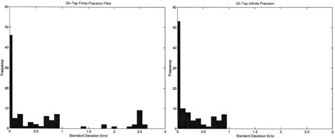
Figure 3-4 shows the frequency distribution of the standard deviation of the error (expected-output) for a infinite precision and finite precision 20-tap filter. Note that even for a channel response that has two samples of post-cursor ISI, the finite-length infinite-precision filter does not converge satisfactory and still has over 48% of the

20-Tap Finite Precision Filter 60 50 -40 30 20 10J 0 0.5 1 1.5 2

Standard Deviation Error

50

40

330

20

ic

20-Tap Infinite Precision

U,_____

2.5 3 0 0.5 1 1.5 2

Standard Deviation Error 2.5

Figure 3-4: Performance comparison of a infinite precision versus finite precision filter. simulated channel responses that has a error standard deviation of greater than 0.1. We note that the finite precision filter have a similar performance, with the exception that it experiences overflow and becomes unstable for some channel responses.

Table 3.2: Examples of channel responses

Behavior Channel response

Converge 0.88282 - 0.1415z-1 + 0.447890z-2

to error std dev <0.1 0.85715 + 0.40270z- 1 + 0.32113z-2

Does not converge 0.82922 - 0.37904z-1 - 0.41075z-2

0.74100 + 0.54183z-1 - 0.39666z-2 Causes tap overflow 0.67690 + 0.39913z-1 + 0.61847z-2

0.74744

+

Table 3.2 shows a snap shot of the channel responses that converges, does not converge, or causes tap-overflow. Note that there does not seem to be any discernible pattern why some converges, some do not, and some causes tap overflow.

3.3.2

Steady State Output Error, Filter Length and Tap

Pre-cision

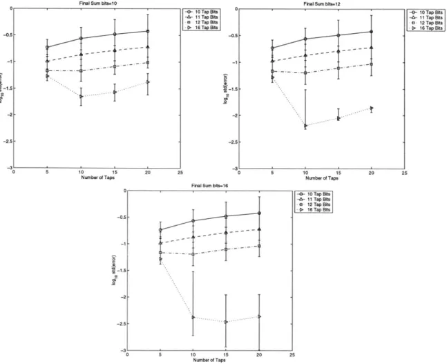
Given the set of channel impulse response that will converge with 20 tap filter, we proceed to see the effects of shortening the filter, and reducing the precision of the taps.

Final Sum blta=12 0 5 10 15 Number of Taps -0.5 -1 -1.5 -2 -2.5 -e- 10 Tap B's -- 1 Tap Bbs a 12 Tap Bbts -> 16TapBIta -0.5 1 -1.5 -2 -2.5 20 25 Final Sum blts=16 I.. 0 5 10 15 Number of Taps

I

.a- 12 Tap Bits

-0 16 Tap Bits

20 25

Figure 3-5: Performance of precision, using round-down

filter with varying tap arithmetic, for ISI over

length, tap precision and adder two time samples.

-0.5 -1 -2 -2.5 -- 10 Tap Bits -f- 11 Tap Bits - 16 Tap Bits 25 20

Final Sum bits-10

A L 4

Final Sum bitsS-1 5 10 15 Number of Taps 20 -9- 10 Tap Bits --- 11 Tap Bits -9 12 Tap Bits - 16 Tap Bits -0.5 -t1.5 -2 -2.5 25

Final Sum bits-16

0, .. -0.5 -1 -15 -2 -2.5 0 5 o10 t Number of Taps 20 0 5 10 15 Number of Taps --- 10Tap Bits

-a- 11 Tap Bits

-e 12 Tap Bits

-* 16 Tap Bits

25

Figure 3-6: Performance of precision, using round-down

filter with varying arithmetic, for ISI

tap length, tap precision and adder over three time samples.

-0.5

-1

-1.5

-2

-0- 10 Tap Bits -A- 11 Tap Bits .e 12 Tap Bits - 16 Tap Bits_ -2.5 F

It....

Final Sum bits-10 10 Tap Bile -- 11 Tap Blie 2- 12Tap BMs 6 1Tap Bits -0.5 -1 -1.5 0 5 10 15 Number of Taps 20 -0.5 _1 -1.5 -2 -2.5 25 0 5 10 15 Number of Taps Final Sum bIts=16

S-e- 10 Tap Bs

-A- 11 Tap Bits

a - 12 Tap Bits - 16 Tap Bits -0.51--1 -2 -2.5 5 10 15 Number of Taps 20 25

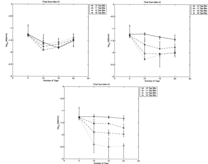
Figure 3-7: Performance of filter with varying tap length, tap precision and adder precision, using round-to-zero arithmetic, for ISI over two time samples.

--- 10 Tap Bits -A- 11 Tap Bits

-6 12 Tap Bits -> 16Tap Bits Final Sum bfts-12 ... . ...

4

+..-.-Using 3 channel responses, we simulated the performance of the filter with varying tap length, tap precision and adder precision. Figure 3-5 shows plots the standard deviation of the error as tap length, tap precision and adder precision is varied.

Refering to the top left graph in Figure 3-5, we make the following observations. First, given the number of taps, and the precision of the final sum, a higher tap precision leads to a smaller error and better performance. Second, a larger number of taps may lead to poorer performance, especially with low precision taps (10,11

and 12). Finally, comparing the three graphs in Figure 3-5, we observe that the precision of the final sum only improves the performance of the filter when the taps have high-precision (in this case 16 bits).

When we performed performed the same experiment with ISI that covers three time samples as shown in Figure 3-6, we found that a larger number of taps led to better performance most of the time.

When we performed the same simulation with toward-zero instead of round-down, the performance of the filter is better, as shown in Figure 3-7. Surprisingly, it is much less dependent on the tap precision, except when the precision of the sum is high.

3.4

Power Consumption of the Baseline LMS

Adap-tive Filter

The power consumption of a baseline six tap filter in Section 3.2 is estimated using Powermill. The precision of the input, taps, intermediate results and outputs were discussed in Table 3.1 and summarized in Figure 3-8. Since the LMS algorithm computes the next tap based on the difference between the current computed output and its expected value, (see equation 2.11) the critical path is from the input a to the tap register, through the output y and the external operation that computes the difference between y and its expected value, and feeds that back as err. Using the results in Table 3.3, assuming that the computation of err requires no time,

the maximum clock rate estimated by Synopsys, using a conservative delay model is

7.196.21 GHz=74.6 MHz.

Table 3.3: Critical path delays.

From To Time (ns)

a[3] (input) y[6] (output) 7.19

err[2] (error input) taps.reg[1][9] (tap register) 6.21

We found correct functionality when clocked at 100MHz. With a power supply of 1.8 volts, the average power consumption is 6.16 milliwatts. The break-down of the power dissipation is shown in Table 3.4. Since we can reduce power consumption in general by decreasing power supply voltage and clock frequency, a more useful metric is to consider the total switched capacitance. The total switched capacitance is calculated using

C = (3.2)

ffV

and equals 19.00 pF. Table 3.5 shows the break down of switched capacitances. We noted that the total switched capacitance of the clock has the same value as the extracted SPICE netlist.

to Dtl Dt2 DO3 Dt4 Dt5

10

ek X + ek X elk X e k X X +ek elk X

10

y[kl : 0

Figure 3-8: Six tap Baseline filter.

3.4.1

Power Dissipation in a Signed Multiplier

In this simulation, we investigate if it is sufficient just to wire the lower-order bits of the inputs to a signed-integer multiplier to zero, if we want to conserve power dissipation by using lower precision taps.

Table 3.4: Breakdown of power dissipation. Element

Total power consumption is 6.16 mW.

[ Percentage I

Table 3.5: Breakdown of capacitances. Element pF

Clock 0.36

Delay line registers 0.91

Tap registers 1.08

Tap update multiplier 5.20 Tap update adder 2.11 Tap multiplier 6.69

Final sum 2.64

7 8 9 10 11 12 13 14 15 16

bits 6 7 8 9 10 bfts11 12 13 14 15 16

Figure 3-9: Power consumption of signed-multipliers of various bit-length given the same 6-bit input.

Clock 1.95

Delay line registers 4.78

Tap registers 5.68

Tap update multiplier 27.37 Tap update adder 11.11

Tap multiplier 35.21 Final sum 13.89 0- nn I -sfet 6- usn I 4.5 3.5 M 2.5 15 0.5 10 0 -f sn -otsgiiaib - sn -es-infiatbt 4 5

Using Synopsys, we synthesized 6, 8, 12 and 16-bit two's-complement signed mul-tipliers. The multipliers were simulated with inputs from a set of 6-bit uniformly generated random numbers. For the 8, 12, and 16-bit multiplier, the 6-bit numbers were placed in the 6 most-significant bits as well as in the 6 least-significant bits (refer to Figure 3-10) When clocked at 100 MHz, with a power-supply of 1.8V, the power consumption, and the total switched capacitance is graphed in Figure 3-9. The results show that in the design of a variable tap-precision filter, using the same multiplier wastes unnecessary power even when the lower-order bits are zeroed. In this case, the power dissipation of a bigger multiplier is bigger because of glitching within the multiplier. In the case of using the least-significant bits of a multiplier, the power dissipation is even greater. This is because the multipliers are two's complement multipliers, so all the higher order bits need to switch when computing the sign and the magnitude of the result.

In the power-scalable filter design to be discussed in the following section, we will allow tap precision to vary in real time. Table 3.6 compares the power dissipation of a 10 by 11 bit multiplier versus a 10 by 16 bit multiplier (using the most-significant bits) given the same set of uniformly distributed 10 bit and 11 bit inputs. By using two different multipliers, when the tap precision changes from 16 to 11, 11% of the energy dissipation can be saved'.

Table 3.6: Comparison of power consumption of a 10 by 11 bit multiplier versus a

10 by 16 bit multiplier given the same set of 10 bit and 11 bit inputs, at a clock

frequency of 100MHz.

10 by 11 bit 10 by 16 bit

Average power [mW] 1.53 1.72

Total switched capacitance [pF] 4.72 5.31

'In our design, we have chosen not to vary the precision of the delay line, as we shall see in the next section. If we chose to vary the precision of the delay line, we would get greater power savings.

6

A[5:0] 6

B:[5:0]

Using least significant bits (s[5] performs sign-extension)

s[5] - A[7:6] s[5] - A[11:6] s[5] A[15:6]

3 A[5:0] A[5:0] A[5:0]

6 6 6

s[5] B[7:6] s[5].J B[11:6] s[5] B[15:6]

B[5:0] ' B[5:0] B[5:0]

6 6 6

Using most significant bits

6 6 6

A[7:2] Z 30: A[11:6] 1 A[15:10]

o A[1:0] 0 3 A[5:0] 0 A[9:0]

6 6 6

B[7:2] B[11:6] 1 B[15:10]

o 4 B[1:0] 0 - B[5:O] 0-- B[9:0]

Figure 3-10: Comparing using large multipliers for small inputs when inputs are placed at the least significant and most significant bits.

3.5

Power-Scalable Adaptive Filter Architecture

Our simulation shows that the major sources are power are the multipliers, followed

by the adders and the registers.

This suggest that we should use burst-mode update of the coefficients, and use power-of-two update. This finding is similar to Nicol et al. [26, 25, 27, 1] as discussed in section 2.2

In addition to dissipating less energy when not needed, we saw that a shorter length can sometimes lead to a smaller standard deviation of error at the output.

We will focus this thesis on making the filter power-scalable. Our findings suggest that significant power can be saved if number of taps and the precision can be varied when necessary.

The design in this thesis will have four levels of adjustability:

1. Level 0 : Five 11-bit taps

2. Level 1 : Ten 11-bit taps

3. Level 2 : Ten 16-bit taps

We have chosen to keep the precision of the delay line constant for this design. We could have reduced the precision of the delay line and this would have given us greater power dissipation reduction.

Based on this discussion, we came up with the following fifteen-tap adaptive filter architecture. Figure 3-11 shows the block diagram of the design. It consists of three 5-tap LMS adaptive filter blocks. Each filter block accepts three inputs: 10-bit input a[k], 10-bit error input e[k], and a 10-bit sum y'[k] from another block. The output

y[kl is the sum of y'[k] and the convolution computed in that block. Each filter block

also outputs a delayed a[n] for the next block. Note that this is simply dividing a 15-tap filter into 3 sections. The three sections are not exactly identical. The first section contains only 4 register banks for the delay line because the first tap does not require a register. The second and third all have 5 register banks. The final filter block does not require to have to have a input y'[n] from another block, so it saves one adder as well. This implementation allows us to shut down the latter two blocks when only 5 or 10 taps are required. In addition, within each block, we can adjust the precision of the taps. We will discuss the implementation of adjustable tap precision in the next chapter. The precision of inputs, taps, intermediate results, and output summarized in Table 3.7. Here we have chosen to increase the tap and output precision from the six tap filter discussed in the beginning of the chapter.

e[n]

e[k] e[k] e[k]

a[n] a[k] y[k-4] a[n-4] a[k] y[k-5] a[n-9]I a[k]

y[n] y[k] y'[k] y2[n] y[k] y'[k] y3[n] y[k]

0 J1 a[k-5]

e[k X elk x elk x elk x elk x

10 1lor 6 x x x x x 11 or 16 7 y[k) + + + y'[k] 10

Figure 3-11: Block diagram of a power-scalable LMS adaptive filter.

Table 3.7: Representation of input, taps, intermediate results and outputs, and the

normalization needed before the next operator.

Variable Representation Normalization needed Input 3.7 or 10#7

-High Precision Taps 2.14 or 16#14

-Low Precision Taps 2.9 or 11#9

-Result of "Tap Multiplier"

High Precision 5.21 or 26#21 Discard two most significant and fourteen least significant bits

Gain of "Normalize 2" = 2-14

Low Precision 5.16 or 21#16 Discard two most significant and nine least significant bits Gain of "Normalize 2" = 2-Input to Sum 3.7 or 10#7

Error Ek 3.7 or 10#7

Aek 10#12

-Result of "Tap Update 1.19 or 20#19 Discard eleven least significant bits Multiplier" _{and sign-extend 2 bits}