Analysis of Demand Variability and Robustness in
Strategic Transportation Planning
by
Ahmedali Lokhandwala
B.S. Marine Engineering
Birla Institute of Technology & Science, Pilani (2007)
Submitted to the Department of Civil and Environmental Engineering and Engineering Systems Division
in partial fulfillment of the requirements for the degrees of Master of Science in Transportation
and
Master of Engineering in Logistics at the
MASSACHUSETTS INSTITUTE OF TECHNOLOGY June 2010
c
Massachusetts Institute of Technology 2010. All rights reserved.
Author . . . . Department of Civil and Environmental Engineering
and Engineering Systems Division May 17, 2010 Certified by . . . . Chris Caplice Executive Director, Center for Transportation & Logistics Thesis Supervisor Accepted by . . . .
Daniele Veneziano Chairman, Departmental Committee for Graduate Students Accepted by . . . .
Yossi Sheffi Professor, Engineering Systems Division Professor, Civil and Environmental Engineering Department Director, Center for Transportation & Logistics Director, Engineering Systems Division
Analysis of Demand Variability and Robustness in Strategic
Transportation Planning
by
Ahmedali Lokhandwala
Submitted to the Department of Civil and Environmental Engineering and Engineering Systems Division
on May 17, 2010, in partial fulfillment of the requirements for the degrees of
Master of Science in Transportation and
Master of Engineering in Logistics
Abstract
Creation of a long-term strategic transportation plan is critical for companies in order to make informed decisions about fleet capacity, number of drivers needed, fleet allocation to domiciles, etc. However, the inherent demand variability present on a transportation network, in terms of weekly occurrences of lane volume, results in emergency weekly shipments that deviate from the long-term plan. This leads to a sub-optimal weekly execution, resulting in higher overall costs, compared to initial projections. Hence, it is important to address this variability while creating a strategic plan, such that it is robust enough to handle these variations, and is easy to execute at the same time. The purpose of this thesis is to create a stochastic annual plan using linear programming techniques for addressing demand variability, and prove its robustness using simple heuristics, so that it is easy to execute at an operational level. Through the use of simulations, it is shown that the proposed planning methodology is within 6% of the optimal solution costs and handles 71% of the demand variability occurring on a weekly basis, making it easy for operational managers to execute. Thus, the proposed plan reduces the optimality gap between long-term planning and weekly operations, creating a tighter bound over the projected versus actual costs incurred, which helps develop a better transportation strategy.
Thesis Supervisor: Chris Caplice
Acknowledgments
I would like to express a deep sense of gratitude and acknowledge the following people for a wonderful journey at MIT for the past two years. I am sure that the list is incomplete, and there are definitely many more folks who have helped me directly or indirectly during my time here.
My mentor and advisor, Dr. Chris Caplice for his constant advice, support and belief in my capabilities over the past two years. His boundless energy, quick think-ing and infallible insights continue to amaze me! He has constantly pushed me to challenge the limits of my capabilities and has been instrumental in my personal and professional growth at MIT.
Dr. Francisco Jauffred, the Principal Investigator on this project (and my office-mate) for his amazing insights and help during my tenure at MIT. Whenever I was stuck with a problem, I knew the solution was only a “question to Francisco” away! No wonder, we lovingly call him the processor that runs the Wal-Mart computer (Francisco Inside!). In addition, I would also like to thank Jeff for his help with the MATLAB codes for my planning scenarios, which have been an instrumental part of my thesis.
My MLOG classmates from the Classes of 2009 and 2010, who have been a con-stant source of inspiration and advice on worldly as well as academic matters. Words cannot express the amount of learnings I have gotten from them - be it during the long hours at the MLOG Lab or the unbelievable amounts of fun that we had outside of it! The good times with them is undoubtedly the part about MIT that I will cher-ish and miss the most! I would also like to mention my friends outside of MLOG, in particular Kushal, Sarvee, Kashi and countless others whose unconditional friendship and help, as well as the long discussions about random topics have made the past two years a memorable experience.
The Administrative Staff from both my programs - in particular, Patty Glidden, Kris Kipp, Ineke Dyer and Mark Colvin who have been of immense help in crossing any administrative hurdles; and Jon Pratt for always being there as a friend and a
supporter, in addition to his help with the recruiting process. The CTL staff on the 2nd floor of E40, particularly Mary, Nancy, Karen & Eric for counting me as a part of the CTL community as well as for all the monthly lunches!
And last, but not the least, I would like to thank my family for their unconditional love and support.
Dedication
I would like to dedicate this thesis to my Mom and Dad for believing in me, and for placing unconditional trust in my abilities and judgement. This thesis has been brought to fruition through your blessings. The values that you have instilled in me are a big part of the person that I am today, and the person that I someday hope to be!
I would also like to share this moment of happiness with my sister Tasneem, brother-in-law Murtuza, my grandparents and in particular, my darling niece Mariya! I cannot thank you’ll enough for always being there for me - through good times and bad.
Contents
1 Introduction 15
2 Trucking Industry Overview 19
2.1 U.S. Transportation System . . . 19
2.2 Transportation Modes and Industry Trends . . . 21
2.3 Trucking Industry . . . 22
2.4 Types of Trucking Fleets . . . 27
2.4.1 Private Fleet . . . 27
2.4.2 For-Hire Carriers . . . 29
2.4.3 Dedicated Fleet . . . 32
2.5 Summary . . . 34
3 Thesis Motivation: Demand Variability and Transportation Plan-ning 35 3.1 Variability . . . 35
3.2 Criticality of Transportation Planning . . . 37
3.2.1 Long-term Planning . . . 38
3.2.2 Short-term planning . . . 40
4 Large-Scale Linear Optimization Model for Transportation Plan-ning 43 4.1 Freight Network Optimization Tool (FNOT) . . . 44
5 The Data and Initial Analysis 57
5.1 Data Consolidation . . . 58
5.2 Lane Demand Distributions & Goodness of Fit . . . 59
5.3 Seasonality in Demand . . . 61
5.4 Correlations in Demand . . . 62
5.5 Sweet Spot on Optimality Curve . . . 64
5.5.1 Metrics . . . 65
6 Planning Methodologies & Weekly Operations 73 6.1 Long Term Annual Planning . . . 73
6.1.1 Stochastic Plans . . . 74
6.1.2 Deterministic Plans . . . 74
6.2 Sub-network used for analysis . . . 75
6.3 Simulation of Weekly Demands . . . 75
6.4 Operational Flexibility Scenarios . . . 79
6.4.1 Complete Operational Flexibility . . . 79
6.4.2 Zero Operational Flexibility . . . 80
7 Simulation Results Analysis 87 7.1 Network Level Metrics . . . 87
7.2 Facility Level Metrics . . . 95
7.3 Tour Level Metrics . . . 99
7.4 Lane Level Metrics . . . 108
8 Conclusions 117 8.1 Opportunities for Future Research . . . 119
List of Figures
2-1 (a) Evolution of the US Transportation Sector in terms of the Value of freight carried; and (b) Evolution of the US Transportation Sector in terms of the Tonnage of freight carried; and (c) Evolution of the US Transportation Sector in terms of the Ton-Miles of freight carried . . 20 2-2 (a) Break-up and evolution of the modes of transportation within the
US in terms of value of freight carried; and (b) Break-up and evolution of the modes of transportation within the US in terms of tonnage of freight carried; and (c) Break-up and evolution of the modes of transportation within the US in terms of ton-miles of freight carried . 23 2-3 (a) Breakup of Revenues generated by the different transportation
sec-tors within the U.S.; and (b) Breakup of Tonnage carried by the dif-ferent transportation sectors within the U.S.; and (c) Breakup of Ton-miles traveled by the different transportation sectors within the U.S. . 25 2-4 Evolution of the types of trucks used for freight carriage . . . 26 4-1 Example of the possible ways in which a load can be moved from Point
A to Point B, at a distance ‘d’ from each other . . . 46 4-2 Example of the distribution of weekly lane demand and the break-down
of demand allocation to fleet versus for-hire . . . 47 4-3 Comparison of a generic Fleet and For-Hire Cost Structure for a single
out-and-back shipment . . . 50 4-4 Optimal Routing in the absence of continuous moves . . . 52 4-5 Optimal Routing when continuous moves are allowed . . . 53
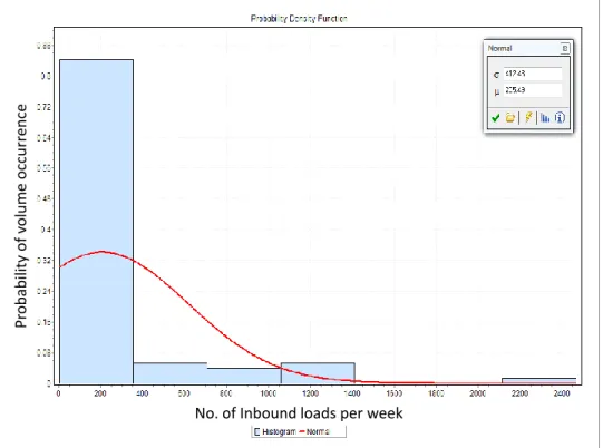
5-1 A Generic Representation of Wal-Mart’s Supply Chain . . . 58 5-2 Aggregated Distribution of all Inbound Lanes from Vendors to a DC
per week . . . 60 5-3 Aggregated Distribution of all Outbound Lanes from a DC to Stores
per week . . . 61 5-4 Change in the No. of Potential Tours generated by the model . . . . 66 5-5 Change in the No. of Tours assigned by the model . . . 66 5-6 Behavior of Total Transportation Costs . . . 67 5-7 Behavior of Tour Efficiency in terms of Percentage Full Loads carried 67 5-8 Behavior of Tour Efficiency in terms of Percentage Loaded Miles . . . 68 5-9 Behavior of Optimality Gap in terms of Total Solution Costs . . . 69 5-10 Behavior of Optimality Gap in comparison to the number of potential
tours generated . . . 70 6-1 Hierarchy of transportation planning - from long-term planning, to
development of weekly operational plans . . . 74 6-2 Example of weekly demand calculation from randomly generated
prob-abilities . . . 77 6-3 An example of demand occurrence during a random week over a tour 82 7-1 Example of a tour with lane details in order to explain metrics . . . . 101 7-2 The graph gives a visual indication of the inverse correlation between
the Actual Probability of Tour Occurrence and the Tour Fickleness factor calculated . . . 102 7-3 Histogram and CDF of Occurrence of All Tours whilst running the
model with Full Flexibility . . . 104 7-4 Histogram and CDF of Occurrence of All Tours occurring within the
Stochastic Annual Plan . . . 105 7-5 The graph indicates that about 71% of tours generated on a weekly
ba-sis within the Full Flexbility operational plan that are already present in the Stochastic Annual Plan . . . 106
7-6 (a) Distribution of the number of freight lanes present in all tours generated in the Full Flexibility Operational Plan; (b) Distribution of the number of freight lanes present in the Stochastic Annual Plan; and (c) Distribution of the number of freight lanes present in all tours generated in the Full Flexibility Operational Plan which are not present in the Stochastic Annual Plan . . . 107 7-7 The graph depicts the distribution of volume occurrence on the lanes
within the network over the 52-week simulation period . . . 109 7-8 The graph depicts the distribution of the lane fleet fickleness factor
over the 52-week simulation period . . . 110 7-9 The graph depicts the distribution of the lane fleet fickleness factor
over the 52-week simulation period . . . 111 7-10 The graph depicts the distribution of the lane fleet fickleness factor
over the 52-week simulation period . . . 112 7-11 Depiction of the use of lane demand statistics as a criterion for lane
List of Tables
2.1 Top ten Private Fleet Owners in the U.S. during 2009 . . . 28
2.2 Top ten TL Carriers in the U.S. during 2009 . . . 30
2.3 Top ten LTL Carriers in the U.S. during 2009 . . . 31
2.4 Differences between Private Fleet, Dedicated Fleet and For-Hire carrier capacity . . . 34
5.1 Correlation Matrix for a Sample DC . . . 63
5.2 Correlation Statistics for a sample DC . . . 64
6.1 Characteristics of the Mini-Network . . . 76
7.1 Summary of Network-level statistics for key metrics . . . 91
7.2 Facility level metrics for DC6006 . . . 97
Chapter 1
Introduction
Trucking plays a pivotal role in the U.S. economy and nearly every good consumed in the country has traveled on a truck at some point. As a result, the trucking industry hauled 68.9% of all freight (in tons) transported in the United States, equating to 9.1 billion tons in 2008(IBISWorld, 2010). The trucking industry amassed an astounding $660 billion in revenue during 2008, representing about 83% of the U.S. commercial freight transportation market (Kirkeby, 2010). Put another way, on average, trucking collected 83 cents of every dollar spent on freight transportation.
Trucks transport the tangible goods portion of the economy, which is nearly ev-erything consumed by households and businesses. However, trucking also plays a critical role in keeping costs down throughout the business community. Specifically, for businesses that produce high-value, low-weight goods, inventory carrying costs can be considerable. But, many of these producers now count on trucks to deliver products efficiently and timely so that they can keep stocks as low as possible. In fact, inventory-to-sales ratios continue to fall, indicating that motor carriers and their cus-tomers are working well together in this area, saving the economy billions of dollars in costs.
The trucking industry is made up of three major types of players:
• Private fleet owners - move cargo solely on privately owned vehicles • For-Hire Carriers - lease trucks to shippers on a short or long-term basis
• Combination shippers - own a private fleet, and supplement them with for-hire capacity
All of these players face the fundamental task of anticipating shipping require-ments and creating a strategic transportation policy to fulfill the demand occurrences at an operational level. Because of the competitive nature of the industry, carriers are under constant pressure to meet service level targets at the lowest possible costs. However, occurrence of demand over a carrier’s network is uncertain in terms of the number of weekly loads to be carried from one point to another. The traditional tools and methodologies commonly used to create the overarching transportation policy do not adequately address this key decision criterion. As a result, this inherent demand variability creates a gap between the forecasted plan for the network and actual weekly execution.
In order to address this gap, there has been ongoing research at the Center for Transportation & Logistics to incorporate demand variability in the transportation planning process, using stochastic planning methodologies. Led by Dr. Chris Caplice and Dr. Francisco Jauffred, the Freight Lab team has created a Freight Network Optimization Tool (FNOT), for deciding the allocation of volume occurrences on a lane to an optimal mix of private fleet and for-hire carriers, as well as finding optimal routes for moving volume over the private fleet. FNOT is a Large-Scale Linear Optimization Model - a detailed discussion about the model and its capabilities is carried out in later chapters. Using the planning scenario created by FNOT, the key questions that this thesis addresses are:
• How do long-term stochastic planning methodologies perform in the presence of demand variability?
• Can simple heuristics be used to reduce the complexity associated with executing a long-term annual plan on a weekly basis?
• What are the key metrics for analyzing the performance of the stochastic plan in comparison to the plans created on the basis of heuristics?
• What are the trade-offs associated with minimizing costs versus simplicity of execution using heuristics?
Thesis Summary
For the purpose of this thesis, we shall analyze Wal-Mart’s transportation network across the continental US. At later stages, we shall pare the network to a smaller sub-section. This serves the purpose of maintaining the overall integrity and charac-teristics of a real-world transportation network, while providing us with a workable data set that can be thoroughly analyzed to draw insights.
We start the thesis by providing an overview of the transportation industry in the US, highlighting the importance of trucking in order to get a better understanding of the major stakeholders within the industry and the issues they face. Having identified the key questions in the previous paragraph, we lay down the motivation behind the thesis by discussing issues related to demand variability and the criticality of planning in transportation. After that, we move into an initial data analysis by sifting through and creating a coherent database, as well as looking for patterns that could potentially explain the demand distributions, seasonality and correlations. This lays down the foundation for creating a long-term annual planning model and testing its performance by simulating weekly demand using Monte-Carlo simulations. The next part of the thesis deals with creating heuristics with varying levels of operational flexibility to figure out ways in which the annual plan can be used to satisfy weekly demand in real-time. The scenarios essentially highlight the difference between the best-case-assignment of demand over the network, versus assigning loads using simple heuristics based on the stochastic annual plan. The analysis compares the weekly execution scenarios using various metrics and throws light on the trade-off between dispatching weekly loads with complete flexibility in the most optimal manner possible, versus executing weekly demand using heuristics based on the annual plan. The analysis is carried out at four levels, in decreasing order of transportation network aggregation. In the process of analyzing these scenarios, we create new metrics that provide a
deeper understanding about the weekly operations and help us get a comparison of the robustness of the annual plan and reasons behind it. Finally, we summarize our findings, discuss the implications and make recommendations for creation of a robust transportation plan that addresses demand variability over the network.
As a slight tangent to the demand variability topic, we also analyze the sweet spot for the trade-off between transportation cost savings obtained by relaxing the constraints on certain run parameters and the computational requirements for running the model.
Chapter 2
Trucking Industry Overview
This section provides a brief overview of the transportation industry within the US. Using statistical data and reports generated over the years, the aim of this section is to provide an insight into the transportation sector and the role that the trucking indus-try, in particular, plays in the overall US economy. In addition, we apprise the reader about the main players within the trucking sector to build a basic understanding of the types of fleet and considerations that go into transportation planning.
2.1
U.S. Transportation System
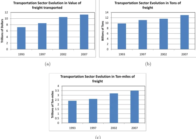
More than 13 billion tons of freight, valued at $11.8 trillion, were transported nearly 3.5 trillion ton-miles in the United States during 2007, according to preliminary es-timates from the 2007 Commodity Flow Survey (CFS)(M. Margreta, 2009). The tonnage, value, and ton-miles of 2007 freight shipments all increased over 2002 totals. Tonnage was up 12 percent, inflation-adjusted value up 13 percent, and ton-miles up 11 percent.
This steady growth in freight movements was possible because of growth in the U.S. economy, an increase in U.S. international merchandise trade, improvements in freight sector productivity, and the availability of an extensive multimodal trans-portation network in the United States. The statistics for historical market trends within the transportation sector are visible in Fig. 2-1.
0 2 4 6 8 10 12 1993 1997 2002 2007 Trill ions of D ollar s
Transportation Sector Evolution in Value of freight transported (a) 0 2 4 6 8 10 12 14 1993 1997 2002 2007 Bill ions of Tons
Transportation Sector Evolution in Tons of freight (b) 0 0.5 1 1.5 2 2.5 3 3.5 4 1993 1997 2002 2007 Trill ions of T on -miles
Transportation Sector Evolution in Ton-miles of freight
(c)
Figure 2-1: (a) Evolution of the US Transportation Sector in terms of the Value of freight carried; and (b) Evolution of the US Transportation Sector in terms of the Tonnage of freight carried; and (c) Evolution of the US Transportation Sector in terms of the Ton-Miles of freight carried
According to the US Department of Transportation(USDOT, 2006), the trans-portation sector moves large volumes of freight to support economic activities in the nation. More than $1 out of every $10 produced in the U.S. Gross Domestic Prod-uct is related to transportation activity. Transportation employs nearly 20 million people in America - 11 million in direct transportation and transportation-related industries (e.g., pilots, train operators, autoworkers, and highway construction work-ers) and another 9 million in non-transportation industries (e.g., truck drivers for retail and grocery stores, wholesale shipping clerks, and distribution managers for manufacturing firms).
On a typical day in 2007, over 35.7 million tons of goods, valued at $32.4 billion, moved nearly 9.6 billion ton-miles on the nation’s transportation network. Nearly 93 percent of the total tonnage and 81 percent of the total value of freight were shipped by means of a single transportation mode, while the remainder was shipped using two or more modes(M. Margreta, 2009).
2.2
Transportation Modes and Industry Trends
Each mode plays an important role in the US freight transportation system - railroads and barges haul bulk commodities and perishable goods over long distances, trucks carry smaller packages to the main streets and back roads of America, and airplanes fly expensive goods overnight across the country. The following discussion is based on the Commodity Flow Survey (CFS) data published by the U.S. Department of Transportation every five years1. Between 2002 and 2007, shipments by trucks grew
the most, measured by value, while rail shipments experienced the highest increase in terms of tons or ton-miles of freight carried. The value of multi-modal shipments increased by 54 percent during this time, followed by increases in pipeline shipments of 51 percent and trucking of 11 percent. By tonnage, multi-modal shipments ex-perienced an increase of 257 percent, followed by rail with 24 percent trucking with
1Source: U.S. Department of Transportation, Bureau of Transportation Statistics, based on
1993, 1997, 2002 and preliminary 2007 Commodity Flow Survey data plus additional estimates from Bureau of Transportation Statistics
18 percent. And by ton-miles, air cargo grew by 63 percent, followed by truck with 56 percent and multimodal combinations by 37 percent. Water transportation ex-perienced a severe downturn during this period, dropping by 78 percent in terms of tonnage and 69 percent in terms of ton-miles of freight carried. A detailed comparison of the modes of transportation in terms of value, tons and ton-miles carried over the years can be seen in Fig. 2-2.
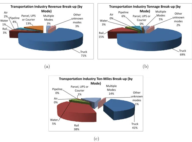
Trucking continued its dominance of the US freight transportation system, as visible in the Fig. 2-3. In 2007, trucks hauled about 71 percent of the value, 69 percent of the tonnage, and 40 percent of the ton-miles of total shipments, exhibiting a positive trend in comparison to 2002 numbers. Measured by ton-miles, trucking was followed by rail at 37 percent and multi-modal at 14 percent. In general, trucking dominated shipment distances of less than 500 miles while rail dominated the longer distance shipments. Multimodal transportation, i.e., shipments moved by more than one transportation mode, grew substantially in value (54 percent) during this period. Of these shipments, parcel, postal, or courier services (typically involving more higher value and smaller size shipments) grew the most rapidly and accounted for over 83 percent of the value of multimodal shipments in 2007. A comparison of the modes of transportation across a variety of metrics is visible in Fig. 2-2.
Thus, it is quite clear that the trucking industry is quite predominant and by far, the biggest and most important mode of transportation for commercial freight within the US.
2.3
Trucking Industry
Trucking is the largest mode in both value of shipments handled and tonnage. Ac-cording to 2007 CFS preliminary data(M. Margreta, 2009), truck shipments accounted for:
• about $8.4 trillion worth of goods, an inflation-adjusted gain of 9.1 percent from 2002, and 71 percent of the total value of all shipments
0% 10% 20% 30% 40% 50% 60% 70% 80%
Truck Rail Water Air Pipeline Multi-modal Other and unknown P er cen tag e Shar e
Mode Comparisons in terms of Value of freight
1993 1997 2002 2007 (a) 0% 10% 20% 30% 40% 50% 60% 70% 80%
Truck Rail Water Air Pipeline Multi-modal Other and unknown P er cen tag e Sh ar e
Mode Comparisons in terms of Tons of freight
1993 1997 2002 2007 (b) 0% 5% 10% 15% 20% 25% 30% 35% 40% 45%
Truck Rail Water Air Pipeline Multi-modal Other and unknown P er cen tag e shar e
Mode Comparisons in terms of Ton-miles
1993 1997 2002 2007
(c)
Figure 2-2: (a) Break-up and evolution of the modes of transportation within the US in terms of value of freight carried; and (b) Break-up and evolution of the modes of transportation within the US in terms of tonnage of freight carried; and (c) Break-up and evolution of the modes of transportation within the US in terms of ton-miles of freight carried
• about 9.0 billion tons of goods, an increase of 14.2 percent from 2002, and 69 percent of all tonnage;
• about 1.4 trillion ton-miles, representing 40 percent of all ton-miles; and • an average distance of 187 miles per shipment
In 2007, trucking (both for-hire and private) continued its dominance of the freight industry, moving 71 percent of the nation’s commercial freight, measured by value, and 69 percent of the tonnage. However, by ton-miles, trucks moved just slightly more than rail, 40 percent compared to 37 percent, followed by multi-modal shipments at 14 percent. These numbers show a faster growth in shipments by truck, compared with rail, and the decline in water transportation since 2002. Truck ton-miles grew by 24 percent, rail by 33 percent, and water declined by about 69 percent. A decade ago, trucks moved almost 28 percent of ton-miles and rail moved about 27 percent, followed by water with 21 percent and pipeline with 16 percent. Fig. 2-3(M. Margreta, 2009) indicates the dominance of trucking in comparison to other modes of transportation, as far as revenues, tonnage and ton-miles are concerned.
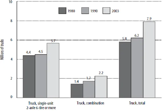
In recent years, as trucking maintained its dominance, the number of trucks travel-ing on the nation’s highways steadily increased and the truck fleet mix changed(USDOT, 2006). While two-axle single-unit trucks are the most common commercial trucks on the nation’s roads, the number of larger combination trucks grew at a much faster rate, increasing about 59 percent over this period, compared to 30 percent for single-unit trucks. In 2003, combination trucks accounted for 28 percent of the commercial truck fleet, up from 24 percent in 1980. These larger trucks also travel more miles per vehicle than the single-unit trucks. Combination trucks generated a total of 138 billion vehicle-miles of travel (VMT) in 2003, compared to 78 billion miles by single-unit trucks. Since 1980, overall truck vehicle-miles have doubled from 108 billion to 216 billion in 2003. Despite this growth in truck VMT, commercial truck’s share of total highway vehicle-miles remained steady, hovering between 7.1 and 7.5 percent over this period. This was primarily because travel by all highway vehicles, including passenger cars, buses, and light trucks (e.g., pickup trucks, sport utility vehicles, and
Truck 71% Rail 3% Water 1% Air 2%Pipeline 4% Parcel, UPS or Courier 13% Multiple Modes 3% Other unknown modes 3%
Transportation Industry Revenue Break-up (by Mode) (a) Truck 69% Rail 15% Water 3% Air 0% Pipeline 6% Parcel, UPS or Courier 0% Multiple Modes 5% Other unknown modes 2%
Transportation Industry Tonnage Break-up (by Mode) (b) Truck 41% Rail 38% Water 5% Air 0% Pipeline 0% Parcel, UPS or Courier 1% Multiple Modes 14% Other unknown modes 1%
Transportation Industry Ton-Miles Break-up (by Mode)
(c)
Figure 2-3: (a) Breakup of Revenues generated by the different transportation sectors within the U.S.; and (b) Breakup of Tonnage carried by the different transportation sectors within the U.S.; and (c) Breakup of Ton-miles traveled by the different trans-portation sectors within the U.S.
minivans) also grew at a similar pace. The evolution of the various types of trucks and their growth is indicated in the Fig. 2-4(USDOT, 2006).
2.4
Types of Trucking Fleets
In order to understand how to create a well conceived transportation policy, it is imperative that the reader have an adequate understanding of how private, dedicated and for-hire carriers differ in terms of cost structures and services provided. This section will provide a high level overview of each of these different types of trans-portation.
2.4.1
Private Fleet
A private fleet is owned and operated by the shipping entity, whose primary business is something other than transportation, such as Wal-Mart, Target, etc. The prin-ciple objective of the fleet is to support the shipper’s internal distribution require-ments. The shipper leases or owns the physical assets such as tractors, trailers and/or straight trucks. The drivers are normally employees of the company. Private carriers are a major part of motor carriage operations. Although little financial information is available on private carriage, the American Trucking Associations estimates that companies running their own shipping operations provided services valued at some $288 billion in 2008, or about 44% of the motor carriage market(Kirkeby, 2010). Ac-cording to estimates from the National Private Truck Council, a trade group, private fleets operate more than two million trucks, make up about 82% of the medium- and heavy-duty trucks registered in the United States, and account for around 56% of all freight tonnage carried by medium- and heavy-duty trucks.
The Table 2.1 lists the ten largest private fleets owned and operated within the US, during 2009, as per FleetOwner.com (2010).
Table 2.1: Top ten Private Fleet Owners in the U.S. during 2009
Private Fleet Owners Total Vehicles Straight Trucks Tractors Trailers
AT&T 78,070 78,000 70 22,000
Verizon Communications 44,973 44,858 115 116
Pepsi Bottling Group 38,500 - -
-Republic Services 22,582 21,960 622 1,378
Waste Management 22,000 20,895 1,105 4,305
Time Warner Cable 18,010 18,000 10 440
Coca-Cola Enterprises 17,400 9,500 7,900 10,000
PepsiCo.’s Frito-Lay 17,109 17,109 -
-Tyco International 15,600 15,600 -
-The ServiceMaster Co. 15,450 15,450 - 1,890
According to Mulqueen (2006), customer service is the preeminent driver of these types of fleets, and is given priority over optimal routing sequences and vehicle uti-lization. Because of the nature of this business, routes are typically constrained more by delivery time than physical space on the vehicle. Optimization is typically used during tactical planning in order to create driver territories and establish route se-quences, but due to the expectation of high service levels, static route planning is often used for daily execution.
For-Hire carriers are usually not considered in these operations due to the need for extremely high level of customer service. Fleets are also much more cost effective than for-hire carriers in these operations due to the high density of low volume stops. This allows a single fleet truck to support the delivery requirements of many of the wholesale distributor’s customers.
Our research is more applicable to shippers that use private fleets for longer haul, full truckload transportation. This is common in many industries including grocery retail (Albertsons, HEB), big-box retail (Wal-Mart, Target) and food/consumer pack-aged goods (CPG) manufacturers (P&G, Kimberley Clark). In this segment, for-hire carriers are often times used to supplement fleet capacity. Typically, for-hire carriers are more efficient due to advantages they hold in terms of economies of scale and scope, however, many shippers still view fleets as an important component in their overall transportation strategy.
As pointed out by Mulqueen (2006), the most common reasons cited for having a fleet include:
• Better perceived service to their customers. Fleet drivers are viewed as impor-tant assets in maintaining a strong shipper/customer relationship.
• Fleet drivers can be requested to perform special services during the delivery that for-hire carriers will not do or would do only for an additional charge. • More leverage with contract carriers during rate negotiations by sending a
mes-sage to the carrier that it can be replaced by an internally managed fleet. • Marketing advantages of having the shipper’s name on the trailer, thereby acting
as a rolling billboard for the company. Provides assurance of freight capacity times of tight capacity, such as exist in the current environment.
• More control over transportation operations.
2.4.2
For-Hire Carriers
The for-hire carrier industry is extremely fragmented, with 240,000 for-hire truck-load carriers in the United States in 2010, of which the top five carriers contribute only 13.5% to the overall industry revenue(IBISWorld, 2010). The activities of this industry can be broadly segmented into consignments weighing greater than 10,000 pounds known as ‘truckload’ and less than 10,000 pounds (less-than-truckload).
Truckload carriers dedicate full trucks to one customer and make deliveries of goods from start to finish. Less-than-truckload (LTL) carriers take partial loads from multiple customers on a single truck and then route the goods through a series of terminals where freight is transferred to other trucks with similar destinations. LTL transportation providers consolidate numerous orders generally ranging from 100 to 10,000 pounds from varying businesses at individual service centers in close proxim-ity to where those shipments originated. Utilizing expansive networks of pickup and delivery operations around these local service centers, shipments are moved between
origin and destination utilizing distribution centers when necessary, where consolida-tion and de consolidaconsolida-tion of loads occurs.
The industry is dominated by truckload carriers. IBISWorld (2010) estimates that more than 80.0% of all establishments are truckload carriers contributing 71.1% of total revenue. LTL is more labor intensive, employing 35.0% of all employees in the industry, costing 40.0% of total wages. This disproportional cost reflects the higher labor intensity of LTL load transport. Revenue is generated per ton hauled; It takes the same labor to ship a 5,000 ton load as 10,000 ton load, but two trips (double the labor) is often required to generate the same revenue.
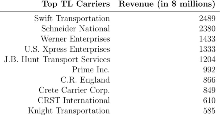
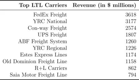
The Tables 2.2 and 2.3 provide the rankings for the top ten TL and LTL Carriers in the US respectively, along with their revenues during 2009 (Schulz, 2010).
Table 2.2: Top ten TL Carriers in the U.S. during 2009 Top TL Carriers Revenue (in $ millions)
Swift Transportation 2489
Schneider National 2380
Werner Enterprises 1433
U.S. Xpress Enterprises 1333
J.B. Hunt Transport Services 1204
Prime Inc. 992
C.R. England 866
Crete Carrier Corp. 849
CRST International 610
Knight Transportation 585
A For-Hire TL carrier is contracted by outside organizations to move freight at a pre-determined rate and operate in environments where loads are greater than 10,000 lbs, which is the approximate breakpoint where the variable nature of LTL costs begin to exceed the fixed nature of TL costs. These carriers pick up freight at the origin point and move it to the final destination without any intermediate loading and unloading of the shipment, although the shipper can contract the TL carrier to perform multiple pickups and/or deliveries under the same bill of lading. This is markedly different from the LTL and parcel transportation network models, which utilize hub and spoke systems that require multiple transfer points to move product
Table 2.3: Top ten LTL Carriers in the U.S. during 2009 Top LTL Carriers Revenue (in $ millions)
FedEx Freight 3618
YRC National 3177
Con-way Freight 2574
UPS Freight 1807
ABF Freight System 1260
YRC Regional 1226
Estes Express Lines 1174
Old Dominion Freight Line 1158
R+L Carriers 862
Saia Motor Freight Line 794
from the origin to the ultimate destination.
The primary benefit of a hub and spoke network is that it enables consolidation of shipments going between terminals. This benefit is not recognizable in a TL environ-ment, since the vehicle is, theoretically, already fully utilized, and injecting a full TL into a hub and spoke network would simply add additional transit time and handling expense to the process.
Additionally, capacity commitments are often specified within TL contracts. From the shipper’s perspective, capacity commitments require the carrier to cover a certain number of loads on a given lane over a specified period of time. This is often done by requesting that the carrier agree to haul a set percentage of total load volume on each lane. This, in theory, provides the shipper the capacity needed to manage the weekly variations in load volumes that a fixed volume commitment would not support.
One important facet of TL transportation that needs to be recognized is that un-like LTL or parcel carriers, For-Hire TL carriers will often reject undesirable loads; even those loads under contract. This occurs if the carrier does not have available ca-pacity or, as carriers get more technologically savvy the load is deemed operationally unprofitable given the current location and status of the carrier’s assets. The fre-quency of carriers turning down loads has increased in recent years as US domestic TL capacity has tightened and the carriers have begun to exert their new found power in the buyer/seller relationship. Harding (2005) showed that the cost of a turndown
was estimated to be between 2% and 7% of the freight spend. In this analysis, over 25% of tendered loads under study were rejected by the primary carrier. The effect of declined freight is discussed extensively by Harding (2005). This tendency of For-Hire carriers increases the uncertainty related to available capacity for the shipper, and can potentially have dire consequences for the latter’s transportation plan. However, for the purpose of this thesis, we shall take the relationships and contractual agreements between the shippers and carriers as a given, and assume that the loads assigned to carriers are never rejected, or are carried by an alternate carrier at the same price.
2.4.3
Dedicated Fleet
Unlike private fleets, dedicated fleets are not owned by the shipper, but are provided on an exclusive basis to the shipper for a contractually specified period of time. Most large Truckload (TL) carriers like Schneider National, JB Hunt, Swift and Werner have active and growing dedicated fleet businesses. The advantages of a dedicated fleet over a private fleet is that a dedicated fleet does not require a large capital ex-penditures outlay as is required when expanding the capacity of a shipper’s private fleet. Dedicated fleets provide the advantages of guaranteed capacity in constrained markets and increased control over the asset and its usage. This has become an im-portant advantage as shippers compete with each other for the available TL capacity on the market (Bradley, 2005).
Like private fleets, shippers will incur dedicated fleet costs regardless of whether the assets are used, since a large component of the cost is fixed versus load based, as in the case of contract carriage. Idle fleet assets and excessive dwell time are especially costly for both dedicated and private fleets. Additionally, the variable component of dedicated contracts typically includes per mile charges that are incurred regardless of whether the vehicle is loaded, thereby penalizing inefficient shippers, as defined by the percentage of empty miles in their networks.
Dedicated and private fleets are both most effective when the shipper has the ability to maximize equipment utilization by minimizing deadhead distance and dwell time as well as by utilizing the assets on shorter-distance runs that incur high
mini-mum fees when executed by for-hire carriers. While there are key differences between private and dedicated fleets, this thesis views them as fundamentally the same. Both modes have significant sunk costs and are perishable in nature in the sense that if the capacity is not used, it is lost. This contrasts with for-hire carriers, which are paid only when used to execute the movement of a load.
Private Fleet and Third Party Freight
A benefit that some companies take advantage of with regard to their private or dedicated fleets is the ability to generate revenue by moving freight for other shipping entities. As the TL capacity in the United States continues to become scarce and rates are driven up, it has become economically compelling for private fleets that have significant empty miles built into their network to acquire common carrier authority and move other shipper’s freight. This industry trend is cyclical, and moves with the macro-economic conditions of supply and demand within the industry. The ability of private fleets to carry third party loads not only helps to generate extra revenue for the company, but also serves to reduce overall empty miles traveled by the fleet and in turn, increases asset utilization. This enables the fleet to generate revenue and turn into a profit center for the shipping organization. This facet of private fleet operation is critical to our thesis. The ability to carry third-party fleet helps private fleet owners reposition their trucks back to the domicile, incurring minimal empty miles along the way. This is done by creating multi-legged tours for the fleet. However, there is a cost versus service trade-off involved in using the private fleet as third party carriers, since overdoing it might affect overall company service levels. This trade-off needs to be kept in mind at all times and freight carriage needs to be prioritized accordingly. The thesis uses a limited application of this ability of private fleet carriers, by allowing them to haul their own freight from vendors to the distribution centers. This serves a dual purpose. On one hand, it helps bring in additional revenue for the company and act as a profit center. On the other hand, it can also be justified from a service stand-point since the fleet is carrying the company’s freight, leading to a more reliable service without compromising on the uncertainty associated with hauling third-party
freight, which might bring in additional demand variability into the network.
Fifty-six percent of private fleets operate with common carrier authority today (Terreri, 2006), although it is not known what percentage of these fleets are actually moving third party freight since there are benefits aside from generating revenue that drive a fleet to attain common carrier authority. For the purpose of this thesis, we do not consider the fringe benefits associated with common carrier authority, and concentrate on it solely as a revenue generating and operational efficiency mechanism.
2.5
Summary
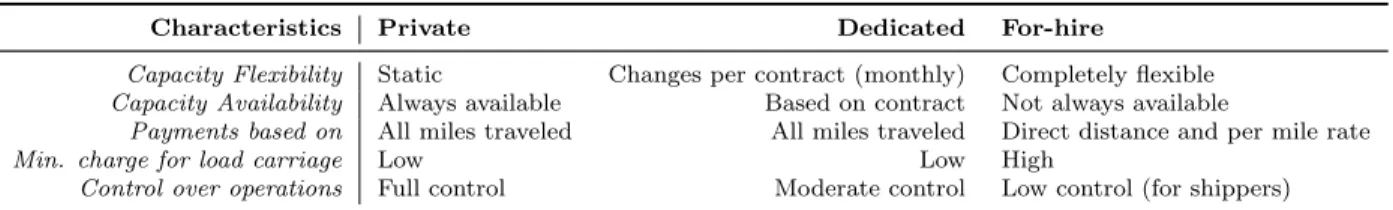
In summary, we can see that the trucking industry is fragmented with a large number of players, because of minimal barriers to entry and exit. We also need to remember that, in practice, all private/dedicated fleet owners utilize for-hire carrier capacity to some extent in order to meet emergency requirements. For the purposes of this thesis, it is critical to note that the private and dedicated fleet pay carriage charges for all the miles traveled by the fleet, while the for-hire carriers charge customers according to the origin-destination distance. In addition, the available fleet capacity for a private fleet at domiciles remains static for a private fleet, change on a periodic basis (based upon contractual agreements) for a dedicated fleet, while it is completely flexible for for-hire carriers. These differences can have significant consequences while creating a transportation plan, and must be taken into account. However, for this thesis, we are assuming that the dedicated fleet and private fleet is equivalent. The Table 2.4 highlights the important differences between private, dedicated and for-hire fleet for the purposes of this thesis.
Table 2.4: Differences between Private Fleet, Dedicated Fleet and For-Hire carrier capacity
Characteristics Private Dedicated For-hire
Capacity Flexibility Static Changes per contract (monthly) Completely flexible Capacity Availability Always available Based on contract Not always available
Payments based on All miles traveled All miles traveled Direct distance and per mile rate Min. charge for load carriage Low Low High
Chapter 3
Thesis Motivation: Demand
Variability and Transportation
Planning
The following chapter provides a synopsis of the types of variability inherent in a transportation network and the importance of addressing demand variability in order to create a robust transportation plan. The need for incorporating these key decision criteria for creating a robust transportation plan is the main motivation behind this thesis.
3.1
Variability
One of the critical aspects that this thesis tries to address is variability. There are many connotations and meanings to the term “variability” - It is derived form of variable which is from the Old French variable, from the Latin variabilis “changeable” from variare “to change”. As far as transportation planning is concerned, variability can occur in three major forms: demand, supply and geography. However, for the purpose of our thesis, we shall only be concentrating on the demand variability, since the remaining aspects of variability do not have a significant impact on the network under consideration.
• Supply variability
This is the type of variability wherein there are constant fluctuations in the avail-ability of fleet or for-hire trucks in order to carry the shipments from one point to the other. This aspect of variability is not a major concern for Wal-Mart be-cause of the large contingent of their private fleet and contractual relationships with for-hire carriers, but could be a crucial consideration for other, smaller shippers.
• Geographic variability
Changes in the distribution network with regard to vendor, distribution cen-ter and store locations can potentially create geographic variability over the transportation network. This would mean that, over time, transportation lanes may be added or removed from the existing distribution network, as demand patterns change. However, this variability has a relatively long time horizon, and hence, is not critical to the planning time frame that we are addressing in our thesis. Thus, we assume a static distribution network that does not change over the time frame for all practical purposes.
• Demand variability
This is the type of variability wherein there are constant changes in the volume of shipments moving on a given transportation lane over a pre-defined period of time, usually assumed as a week. This aspect of variability can have tremendous impacts associated with creating a strategic plan for long-term fleet capacity as well as developing contracts with third party carriers.
For the purpose of this thesis, demand variability is the most critical aspect, and shall be dealt with in detail. Most contemporary off-the-shelf software tools neglect this aspect of variability and instead use a single value of ‘average loads per week’ for planning purposes. However, the underlying variability on the lanes leads to executional strategies that are quite different in reality.
The following thesis particularly addresses planning problems faced by combina-tion carriers, who own a private fleet, and use for-hire carriers to supplement their capacity. Thus, they basically incur a fixed cost associated with the private fleet, and variable for-hire costs for having flexible capacity for meeting demand fluctuations over the year. The two classic cases that could be the result of demand variability for these shippers are discussed below:
• Actual demand is higher than planned
This would lead to short-term dependence on for-hire carriers to carry the freight, which would have a dual impact. Firstly, for-hire carrier charges would be a lot more for hauling freight on an ad hoc basis. Secondly, there would be uncertainty associated with the availability of for-hire carriers on a short-term basis, which would directly affect service levels.
• Actual demand is lower than planned
This would lead to under-utilization of the private fleet and would affect the shipper in the form of wasted sunk costs related to idle fleet and driver capacity. Typically, over the course of the year, both of these cases will occur multiple times because of demand variability creating volume fluctuations with respect to the planned capacity. Thus, in order to mitigate these losses, unexpected, short-term decision making takes place at an operational level, which leads to system sub-optimality. These decisions create a wide gap between predicted costs during long-term strategic planning and actual costs incurred. Additionally, this short-long-term sub-optimal decision making might also affect overall company service levels, in cases where demand cannot be met in time. One of the major points that this thesis is trying to address is to minimize this gap between planning and execution.
3.2
Criticality of Transportation Planning
Because of the inherent variability in transportation demand, creating a transporta-tion policy that at least closely simulates real-time operatransporta-tions is quite critical. The gap
between planning and execution can be addressed by creating a robust transportation policy that gives due consideration to variability over the distribution network and proposing a plan that is as close to real-life execution as possible. This plan should be capable of incorporating the operational uncertainties associated with demand, as a criterion for decision making. The tools and methodologies currently available do not adequately address this key decision criterion for creating an overarching trans-portation policy, which is the main motivation behind the research carried out in this thesis.
Transportation planning must be capable of satisfying long-term as well as short-term decisions effectively. Let us consider the decisions that companies hauling freight by using a mix of privately owned fleet and for-hire carriers need to make, in the long as well as the short-term.
3.2.1
Long-term Planning
This level of planning is required for deciding the overall transportation strategy of a company. The time horizon associated with these decisions could be anywhere between one to five years. Long term decisions usually have large amounts of capital expenditure and sunk costs associated with them. Hence, having a robust long term plan that would be operationally viable would help a company in the following ways:
• Making decisions for expenditure related to fleet acquisition
Depending upon the demand variability over the transportation network and policies related to satisfying demand using the private fleet, a company needs to decide upon their fleet size. Also, since the average life span of a truck is around five years, this decision needs to be robust, in order to utilize the fleet efficiently in the long run.
• Allocation of fleet to distribution centers based on tour plans
Depending upon the long-term projected demand flowing into or out of a dis-tribution center, a decision needs to be made for allocating fleet capacity to the DC, such that it is capable of handling demand requirements adequately.
• Fixed/ Sunk costs associated
There could be fixed or sunk costs related to construction of shipping docks and other miscellaneous expenses that need to be taken depending upon the transportation requirements.
• Hiring of Drivers
Since driver salaries are a fixed cost, the hiring decision heavily depends upon the projected utilization that a company hopes to get out of their drivers. Idle drivers lead to a lot of wasted resources, and hence, this decision needs to be made carefully. In order to mitigate these losses, most firms have a mix of full-time employees based on long-term demand patterns and contract-based employees to satisfy demand fluctuations in the short run.
• Long Term contracts with for-hire carriers to get better rates for spe-cific lanes
In order to ensure that a company gets the best for-hire lane rates, it is im-portant to build long term relationships and contracts with the carriers. If a load is assigned to a for-hire carrier on an ad-hoc basis, they might qualify the load as an emergency shipment, and charge a high amount to move the load. If the contracts for load carriage by for-hire carriers are made well in advance, it would not only ensure that a for-hire truck is available whenever needed, but would also enable the company to get lower rates.
3.2.2
Short-term planning
After figuring out the long-term planning decisions for the transportation network, a short-term plan is needed to make the daily or weekly decisions for operational managers, in order to ensure optimal utilization of available resources. The two main decisions that need to be made over a short-term are:
• Allocation of available fleet capacity to optimal routes, based on weekly demand
Thus, depending upon the demand, the operational managers need to make a decision on how to route the private fleet in the most optimal manner such that the loads are moved in the most cost-effective way and meet the requisite service level targets set by the company.
• Short term allocation of capacity to for-hire in order to meet unmet weekly demand
In cases where demand fluctuations are so heavy that the load occurrences cannot be satisfied by the private fleet, the operational managers need to make alternate arrangements for moving the load, using short-term for-hire contracts.
Demand variability has a huge role to play in the short-term as well as long-term decision making process. If the variability is not handled effectively by the trans-portation plan, there tends to be a significant gap between the expected plans and the actual operations. This divide leads to extra costs and low service levels at the operational level.
Hence, there is an inherent tradeoff involved between
-• Optimizing a complex transportation plan to generate maximum theoretical savings by creating best possible scenarios on an everyday operational basis
• Adequately addressing the uncertainties, and creating a simplified plan that is easy to execute
It is our hope that the proposed techniques in this thesis shall balance this trade-off and help create a robust long-term transportation plan that actually materialize in practice, by taking the demand uncertainties into account.
Chapter 4
Large-Scale Linear Optimization
Model for Transportation Planning
Mulqueen (2006) laid down the groundwork regarding the importance of addressing demand variability while creating a transportation policy. He created a two-step strategy for transportation planning - the first part involved creating a deterministic linear programming model to assign volumes to tours based on user-defined confi-dence levels; the second part of the strategy involved testing the optimization results with random demand simulations in order to understand the behavior of the deter-ministic optimization policy in a real-life scenario. This comparison indicated that the savings predicted by a deterministic transportation policy were highly dependent upon user-defined confidence intervals and hence, not robust enough to emulate real life scenarios. These results were crucial in reiterating the true stochastic nature of transportation lane volumes. The shortcomings pointed out by Mulqueen (2006) led to further research into the area and paved the path for creation of the Freight Net-work Optimization Tool (FNOT), which forms the base of this thesis. The following chapter provides a high-level summary of the methodology used by FNOT for creat-ing a transportation policy that addresses demand variability. In the first part, we discuss the allocation of lane volume to an optimal mix of fleet and for-hire carriers. In the next part, we discuss the formation of tours for volume to be carried over the private fleet.
4.1
Freight Network Optimization Tool (FNOT)
Realizing the importance of addressing demand variability in transportation networks, there has been ongoing research at the Center for Transportation & Logistics at the Massachusetts Institute of Technology for developing a tool that addresses this uncer-tainty. Led by Dr. Chris Caplice and Dr. Francisco Jauffred, the Freight Lab team has come up with a Linear Programming Optimization model called the Freight Network Optimization Tool (FNOT)(F. Jauffred, 2010). FNOT is basically is a steady state model that conducts large scale linear optimization. The objective of the model is to assign shipments over the distribution network at an optimal mix of private fleet and for-hire carriers while minimizing the overall costs for the network. Additionally, in order to reduce the number of empty miles travelled by the private fleet within the network, the model also looks for tours (a set of continuous moves for the fleet) that can satisfy lane demand in the most cost-effective way, and assigns the lane vol-ume accordingly. In order to address the demand variability aspect, FNOT has the capability of modeling the demand distributions over the transportation lanes using stochastic distributions like Normal, Poisson, etc. as well as by using histograms of demand formulated from empirical data. Furthermore, FNOT also has the capability of breaking down a freight lane into a set of two or more moves, called relays, if it is cost-effective to do so. Unlike Mulqueen’s multi-stage optimization and simulation approach, FNOT integrates stochastic conditions within the optimization method-ology to find the optimal transportation policy that takes demand uncertainty into account.
4.2
Understanding FNOT
The objective function behind the FNOT engine is to minimize total transportation costs over the distribution network while optimally assigning volumes to the private fleet and for-hire carriers, based on some supply-demand constraints.
Objective function: Minimize (Total Fleet Costs + Total For-Hire Costs + Relay Costs)
Subject to the constraints:
• All lane volume must be satisfied by either fleet or for-hire
• Fleet assignments must not exceed available fleet or driver capacity
• Actual lane volume assigned by the model to private fleet must be between the overall minimum and maximum values of lane demand
FNOT assigns lane volume to a mix of fleet and for-hire carriers in a unique manner. This calculation is carried out using a modification of the Newsvendor formulation for transportation planning purposes. The essence of this calculation is the use of loss functions for for-hire volume assignment. In statistics, a loss function represents the loss (cost in money or loss in utility in some other sense) associated with an estimate being different from either a desired or a true value, as a function of a measure of the degree of deviation (generally the difference between the estimated value and the true or desired value). In our case, the loss function represents the degree with which our estimate about volume planned on a lane to be covered by private fleet is lower than the actual volume occurring on the lane, i.e. the expected volume not covered by the private fleet. As such we have to incur a penalty by fulfilling the remaining demand using for-hire carriers, and thereby paying an extra cost to them over and above what was originally planned for.
Let X be the optimal fleet demand allocation point on the empirical histogram. That is, whenever demand occurs on this freight lane which is less than or equal to X, it makes economical sense to assign the loads to private fleet, and all demand above it should go to for-hire carriers. The value of X would be our final decision in creating
a volume assignment plan for fleet and for-hire carriers for this transportation lane. The underlying question is, “How do we find X?”
A
B
Indicates Private Fleet Tour carrying load from A to B, and returning empty from B to A
Indicates load carried by For-Hire Carrier from A to B
Loaded Leg of Tour
Empty Leg of Tour
Figure 4-1: Example of the possible ways in which a load can be moved from Point A to Point B, at a distance ‘d’ from each other
For the sake of simplicity, let us consider the example shown in Fig. 4-1, consisting of a transportation lane from point A to B. Demand occurring on this lane over a particular week can be transported by using either the private fleet or a for-hire carrier option. The private fleet option would be to send a truck from A to B and bring it back to A empty. The second option would be to use a for-hire carrier to ship the load.
This lane has an empirical histogram of demand information, as shown in the Fig. 4-2 (Note, that FNOT is capable of producing the same analysis using probability distributions as well). The histogram presents a pictorial representation of the portion of lane volume that shall be carried over the private fleet, with the excess demand (beyond X) assigned to for-hire. This allocation is obtained by comparing the costs for carrying the load using private fleet with for-hire carrying costs, in conjunction with the demand information available through the histogram.
Let
0 4 8 12 16 20 0 4 5 6 7 8 9 No . of W ee ks
Volume carried on the lane
Empirical Distribution of Lane Demand
(Example)
X*
Lane Demand Carried by Private Fleet Lane Demand Carried by For-Hire Carriers
Figure 4-2: Example of the distribution of weekly lane demand and the break-down of demand allocation to fleet versus for-hire
d = Distance between points A and B (miles)
p = For - Hire cost per mile for carrying a load from point A to B ($ /mile) X = Planned optimal fleet demand allocation point
D = Actual value of demand on a lane
P (D > X) = Probability that the actual demand occurring on the lane is greater than X
In the event that demand for the lane is less or equal to the fleet planned volume, the entire demand can be satisfied by the private fleet.
Hence,
Total Transportation Cost = Fleet Cost = 2cdX
the excess demand needs to be satisfied using for-hire carriers. Hence, Fleet cost = 2cdX For-Hire cost = pd ∞ R X P (D > ψ)dψ
Total Transportation Cost (TTC) = Fleet Cost + For - Hire Cost
= 2cdX + pd
∞
Z
X
P (D > ψ)dψ
As per the definition of Loss function discussed previously, the extra costs related to meeting the unplanned excess demand on the transportation lane corresponds to for - hire carriage costs. This loss would only be incurred if the planned optimal fleet demand allocation is smaller than the actual demand occurrence.
Hence, the loss function formula can be generically stated as,
Loss function = E[max(0, D − X)] = pd
∞
R
X
P (D > ψ)dψ
As per the Newsboy Equation, the optimal point would occur when the Total Trans-portation Cost function reaches its minimum; i.e.,
Marginal Cost of Private Fleet - Marginal Cost of For - hire carriers = 0
∂ ∂X(2cdX) − ∂ ∂Xpd ∞ R X P (D > ψ)dψ = 0 2cd − pdP (D > X) = 0 P (D > X) = 2cp
Using this probability value, the optimal X can be easily figured out from a cumulative empirical distribution of lane demand that we possess, as shown in Fig. 4-2. The Loss function is continuous and convex for all positive values of X thus the total
transportation cost, TTC(X), is continuous and convex in the same domain. In consequence TTC(X) always has at least one optimal minimum value.
Intuitively, this formulation makes sense as well. Marginal costs are defined as the change in total cost incurred when the quantity produced increases by one unit. In our case, the marginal costs for private and for-hire fleet can be considered as the effect that one extra capacity over the private fleet or for-hire carriers has, on the total costs of the network. When demand is below optimal (X), we have idle fleet capacity that adds to the total costs, since it is not fully utilized. When demand is above optimal, we have to incur costs related to allocating the excess demand to for-hire carriers. Hence, the only way we can have minimal impact on the total cost equation is to obtain the condition where we are indifferent between having an extra capacity of fleet or for-hire carriers available to us, since our demand is being met optimally by the private fleet, i.e. marginal costs of private fleet equals marginal costs of for-hire carriers. Thus, generalizing the discussion, we can say that the allocation of freight to for-hire carriers depends on the loss function of the demand distribution. We know from the calculations above that demand allocation to fleet or for-hire carriers is essentially dependent upon the costs associated. Hence, let us consider the extreme cases for fleet versus for-hire costs, and see how it affects our assignments.
Case 1: For-Hire costs (p) are substantially higher than Total Fleet Costs (2c)
Hence,
2c
p ≈ 0 ⇒ P (D > X) ≈ 1
Therefore, all demand occurring on the lane would be assigned to the private fleet.
Case 2: For-Hire costs (p) are substantially lower than Total Fleet Costs (2c)
Hence,
2c
Therefore, all demand occurring on the lane would be assigned to the for-hire carriers.
After deciding the optimal loads on all freight lanes within the network, the next part of the model deals with trying to find continuous moves for the private fleet over the network, to further minimize the costs.
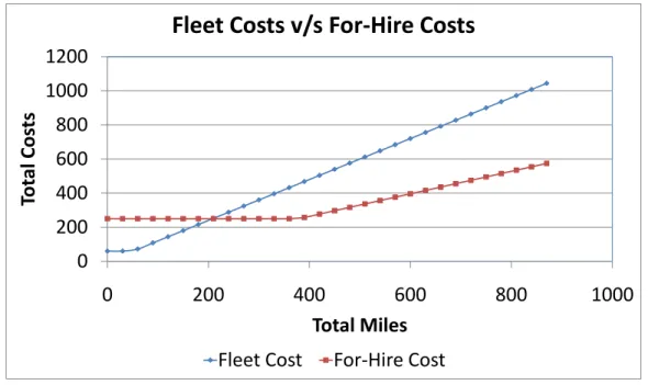
If we were to consider using a private fleet solely for out-and-back moves (as illustrated in the example shown in Fig. 4-1), we place a great limitation on the effective use of the private fleet to carry loads over longer distances. This is because of the cost structure generally used in the transportation industry for private fleet and for-hire carriers. The behavior of a generic fleet and for-hire carriage cost structure with respect to distance traveled over a lane is indicated by the Fig. 4-3.
0
200
400
600
800
1000
1200
0
200
400
600
800
1000
Tot
al
Cos
ts
Total Miles
Fleet Costs v/s For-Hire Costs
Fleet Cost
For-Hire Cost
Figure 4-3: Comparison of a generic Fleet and For-Hire Cost Structure for a single out-and-back shipment
This dictates that for-hire carriers would make more economic sense if we were to compare them to any out-and-back tours that are longer than 95 miles (one way). The reason is that, for out-and-back tours, 50% of the tour cost is incurred because of empty miles travelled by the fleet in order to return to its origin. However, if we
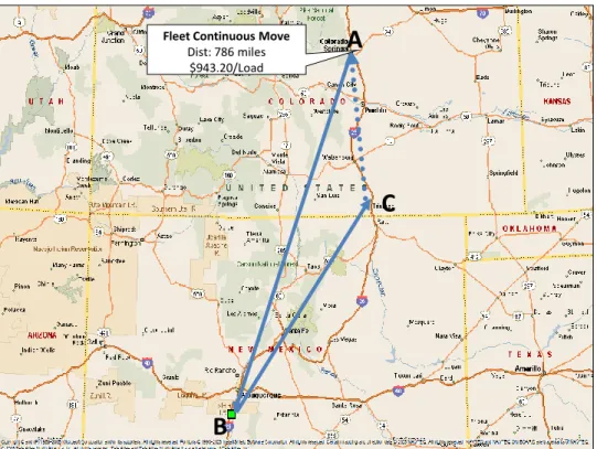
were to somehow find other possible lane volumes that the fleet could satisfy through continuous moves, we could minimize the overall empty percentage miles travelled by the truck. This would make a strong case for allocating more loads to the private fleet and increase asset utilization simultaneously. For the example shown in Fig. 4-4, if continuous moves are disallowed over the network, the optimal allocation for volume occurring over the network is broken down into a for-hire move (A-B) and an out and back tour (B-C-B). The associated costs are:
A-B: Carrier costs, which would be the maximum of $250 (minimum amount charged by the for-hire carriers for carrying this load) and distance times the for-hire rate per mile based on the carrier bid ($2.21 per mile for this lane). The distance traveled over this lane is 368 miles, which results in for-hire costs of $813.28 per load.
Carrier Cost = Max[250, Distance X For - Hire Cost per mile]
Carrier Cost = Max[250, 544 X $ 2.21] = $ 813.28
B-C-B: Private fleet costs are calculated as the total distance traveled by the fleet times the per-mile fleet costs incurred by the company. The distance from B-C is 272 miles. Hence, the total fleet costs for the tour B-C-B would be the maximum of out-and-back distance times the per-mile fleet costs and the minimum charge for moving a load ($50, as decided by the private fleet owners). This leads to the overall tour costs equating to $652.80 per load.
Fleet Cost = Max[50, Distance X Fleet Cost per mile]
Fleet Cost = Max[50, 272 X 2 X $ 1.2] = $ 652.80
Thus, for this example, the overall costs to the company for moving the two loads over the network would be $813.28 + $652.80 = $1466.08.
However, when continuous moves are allowed, both loads can be carried by a private fleet truck on a tour A-B-C-A, as shown in Fig. 4-5, wherein the truck has to travel empty from C-A. At the fleet rate of $1.2 per mile, the overall costs for carrying