Defects in liquid crystal polymers : their origins and behavior in magnetic and flow fields

DEFECTS IN LIQUID CRYSTAL POLYMERS:

THEIR ORIGINS AND BEHAVIOR IN MAGNETIC

AND FLOW FIELDS

by

Janelle Gunther

Submitted to the Department of Materials Science and

Engineering

Program in Polymer Science and Technology

in partial fulfillment of the requirements for the degree of

Doctor of Philosophy

at the

MASSACHUSETTS INSTITUTE OF TECHNOLOGY

June 1997

© Massachusetts Institute of Technology, 1997. All Rights Reserved.

Author ...

...

Janelle Gunther

May 2, 1997

Certified by

...

/

Edwin L. Thomas

Morris Cohen Professor of Materials Science and Engineering

Thesis Supervisor

Accepted by

...

Linn W. Hobbs

John F. Elliott Professor of Materials

Chairman,

Departmental Committee on Graduate Students

.,vASSACHUS,"TS INST'; u :

OF TECHNOLOGY

-SCINCE

DEFECTS IN LIQUID CRYSTAL POLYMERS: THEIR ORIGINS AND BEHAVIOR IN MAGNETIC AND FLOW FIELDS

by

Janelle Gunther

Submitted to the Department of Materials Science and Engineering Program in Polymer Science and Technology

on May 2, 1997,

in partial fulfillment of the requirements for the degree of Doctor of Philosophy

Abstract

Pattern formation and evolution in liquid crystal polymers is studied in both static situa-tion as well in applied magnetic and flow fields. Observasitua-tions of nucleasitua-tion and growth of nematic domains in an isotropic matrix under static conditions were used to establish the origins of the most common types of point defects. The patterns describing the director field distribution were revealed using a solidification induced banding method on

quenched samples. At a low percent conversion of isotropic to nematic, the defect density is dominated by domain density and by anchoring conditions between the nematic

domains and the isotropic matrix. At higher percent conversions, the defect density is con-trolled by domain-domain interaction events. The defect density rises as the domains nucleate and impinge but decreases after the generation of defects of negative strengths and an annihilation process begins. Larger domains created in the coalescence process can then grow and impinge and continue defect generation via domain interaction. The absence of negative strength defects during the preimpingement phase indicates these defects arise solely due to the domain-domain coalescence during the growth process. The subsequent effects of both magnetic fields and flow fields on defect structure are also examined. With respect to the former, a solution of the director orientation distribution function is presented for N6el inversion walls created in a liquid crystal by application of a magnetic field. The theoretical model is used to simulate director trajectories across walls as a function of both the elastic anisotropy and the orientation of the wall with respect to the applied field. The gradual transition of the defect structures from Neel bend walls to Neel splay walls as the angle between the wall and the magnetic field is varied is also pre-sented. Experimental micrographs obtained via atomic force microscopy on a thermotro-pic liquid crystalline polymer are used to test and evaluate the theoretical model.

Visualization of director textures using the lamellar decoration technique shows the theo-retical and experimental results to be in good agreement. The results were used to deter-mine that the sample had an elastic anisotropy of 0.5, implying that k, = 3k ₃₃

The effects of flow on the disclination textures were studied with an optical shearing cell. Flow visualization experiments were used to study curvature driven motion in disclination loops created during flow. Theories of differential geometry were used to predict the way the line curvature should evolve over time. Theoretically the relationship between velocity and local curvature is linear. Experimentally, deviations from the theory sometimes occurred due to forces of attraction between nearby disclinations. Even though disclina-tion evoludisclina-tion in both small molecular and polymer liquid crystals obeyed similar physical laws, several significant differences were observed. Disclinations in the polymer systems generally displayed initially highly contorted contours. In the small molecule liquid crys-tals however, the loop contours consistently displayed very simple shapes. In the polymer system, the complex line shape reflects the many prior loop-loop coalescence events due to the greater density of loops than in the low molar mass liquid crystal. Moreover, the reduction of regions of high loop curvature is inherently slower in the polymer liquid crys-tal due to the higher viscosity of the medium. In addition, the motion of the disclination contour may also be affected by a possible reduction in the mobility of disclinations due to the presence of lower molecular weight components at the defect core which themselves must diffuse along with the line defect.

Thesis Supervisor: Edwin L. Thomas

Acknowledgments:

It is hard to believe that my 8+ years at MIT are coming to an end! Before departing there are many people I would like to thank. First I would like to express my appreciation to my advisor Professor Edwin Thomas, for his enthusiasm and support over the years. His excitement for scientific research made an indelible impression on me when I came to him as a sophomore in September of 1989 to inquire about undergraduate research oppor-tunities in his group. Since that time he has taken great care in my professional develop-ment, something that has added significantly to my positive experience at MIT. As I reflect on the last 8 years I have worked for him, I am beginning to understand the advice given to me by one of his former students. One person in particular suggested that if I wanted to start research as a undergraduate I should "go work for Ned Thomas". That was it. No "ifs", "ands" or "buts", just "do it". When I look back now, if I had to do it over again I wouldn't have done anything differently. The lessons I have learned from Ned about aca-demics, research, and group management are invaluable and will serve a foundation for

some day in the future when I start my own research group.

I am also very grateful to Professor Michael Rubner for his support, especially of my desires to become involved with teaching. The first time we worked together was in the Fall of 1992 when I was a grader for his course in Polymer Chemistry. He gave me his full support when I expressed an interest in also running review sessions and holding office hours in addition to my regular duties. I was honored when he asked me to become a full-time graduate teaching assistant for him in the fall of 1995. The marvelous example he set in the classroom is something to which I aspire. His continued advice over the years is something that I have appreciated a great deal.

There are many other people that have been instrumental in my career at MIT. I am very grateful to Professor Robert Rose for his guidance and support over the years. He has been one of the most influential professors I have interacted with and has been instrumen-tal in my decision to become a professor.

I would also like to thank the members of my committee: Professors Robert Arm-strong, Ken Russell and Chris Scott for their advice and suggestions. Professor Sam Allen was also very instrumental in my research on curvature driven motion of disclination loops. Scott Clingman (Cornell University, Professor Chris Ober's group) was a main driving force in this research through the superb polymers he synthesized for me. I don't know what I would have done without him. I owe you one Scott!

I also could not have done this without the continual support of my friends and family. I would like to thank Leslie Lawrence, Marshall Hughes, Dongsik Yoo and Barbara Dirsa for their friendship over the years. A big thank-you is also due to Kevin McGinty, my piano teacher, who was not only a superb teacher but a good friend as well. He was one of the main people who helped me maintain my sanity while finishing my degree. The love and support of my parents, Paul and Lynda Gunther, helped pull me through the difficult moments. To all my brothers and sisters: Jordan, Jenessa, Jilenne, Julia, Jansen, Justus, and Jesse...yes! I am now Dr. Gunther! I am deeply indebted to my brother Jordan who spent nearly one week of his summer vacation helping me finish the final corrections on my thesis. I couldn't have done it without you! Finally, I would like to thank the Lord for his love and blessings and without whom none of this would have been possible.

Table of Contents

A bstract ... ...

Acknow ledgm ents: ... ... 4

Table of Contents ... ... 5

List of Figures ... ... 7

L ist of Tables ... ... 16

Chapter 1 Background On Liquid Crystals...17

1.1 A pplications ... ... 17

1.2 Introduction... 18

1.3 Defect Structures in Nematic Liquid Crystals ... ... 21

1.3.1 Defect Morphology ... ... 21

1.3.2 Defect Interaction... ... 25

1.3.3 Non-Equiconstant Case... ... 27

1.4 Static Situation in Two-Dimensions -Schlieren Textures...28

1.5 The Effect of Magnetic Fields on Defect Textures... ... 28

1.6 The Effect of Flow Fields on Defect Textures... ... 29

1.6.1 Defect Walls formed by Flow Fields ... 29

1.7 Disclination Loops and Threads ... 32

1.8 Liquid Crystal Rheology... ... 32

1.8.1 Leslie-Ericksen theory ... 32

1.8.2 Shear Flow of Nematics ... 34

1.8.3 Tumbling and Flow Aligning Nematics ... ... 35

1.8.4 Shear Flow Visualization ... 36

1.9 Introduction to the Thesis ... ... 40

Chapter 2 Experimental Techniques ... 62

2.1 Introduction... ... 62

2.2 Light M icroscopy ... ... 62

2.2.1 Use of Compensators ... 63

2.2.2 Solidification-Induced Banding ... 64

2.3 Atom ic Force M icroscopy ... 64

2.4 Optical Shearing Apparatus ... 65

Chapter 3 Defect Generation Mechanisms ... ... 74

3.1 Introduction... ... 74

3.2 B ackground ... ... 74

3.3 Determination of Anchoring Conditions ... ... 77

3.4 M aterials ... ... 79

3.5 Experim ental Procedure... ... 79

3.6 Early Stages of Domain and Defect Development ... 80

3.7 Middle Stages of Domain and Defect Development ... .... 81

3.8 Late Stages of Domain and Defect Development...81

3.8.1 Formation of the s= -1 defect... ... 82

3.8.2 Formation of s=- 1/2 defects ... 83

3.8.3 Formation of the s=+1/2 defect... 85

3.8.5 Implications for Materials Parameters ... ... 86

3.9 Sum m ary ... ... 86

Chapter 4 Computer Simulations of Static Defect Textures... ... 115

4.1 Introduction ... 115

4.2 B ackground ... 115

4.3 Computer Methods... 118

4.4 Director trajectories and Polarized Light Simulations for Individual Point Defects. 119 4.5 Repulsion of Defects of Similar Sign: A single s=+2 or two s=+1 Defects? .. ... 119

4.6 Defect Generation Mechanism Experiments, Computer Simulations and the Implica-tions for Defects of High Strength... 122

Chapter 5 The Effect of Magnetic Fields on Defect Structure ... 153

5.1 Introduction... 153

5.2 Theoretical Background...154

5.3 Sample Preparation ... ... ... 160

5.4 Results and Discussion ... 161

5.5 Summary ... 164

Chapter 6 Curvature Driven Motion in Liquid Crystal Polymers... 181

6.1 Introduction... 181

6.2 Curvature Driven Motion...181

6.2.1 Background...181

6.2.2 Mathematical Algorithms for Studying Curvature Motion ... 187

6.2.3 Introduction... ... 187

6.2.4 Algorithms of Differential Geometry -The Marker Method... 188

6.2.5 Algorithms of Differential Geometry -The Level Set Approach... 188

6.3 Evolution of Disclination Loops in Liquid Crystals ... 189

6.3.1 Introduction ... 189

6.3.2 Experimental Procedure ... 191

6.3.3 Experimental Results ... 192

6.4 Curvature Measurement Algorithms... 193

6.4.1 Introduction ... 193

6.4.2 Error Analysis ... 194

6.4.3 Curvature Motion in Liquid Crystals ... 196

6.5 Sum m ary ... 199

Chapter 7 Sum m ary ... ... 227

7.1 List of Conclusions ... ... 227

7.1.1 Defect Generation Mechanisms ... ... 227

7.1.2 Magnetic Field Effects ... 227

7.1.3 Curvature Driven Motion of Disclination Loops...228

7.2 Thesis Research ... ... 228

List of Figures

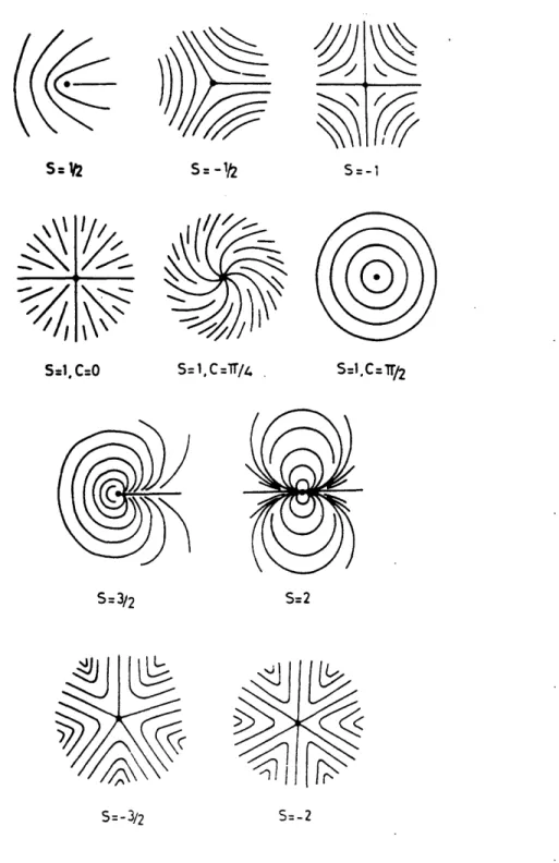
Figure 1.1: This schematic emphasizes the interconnections between structure, properties, processing and performance. The defect placed at the center of the pyramid can have a strong influence on all the other parameters ... 47 Figure 1.2: a) A schematic depicting a rod-like liquid crystal with mesogens in the chain. b) A similar material but with the mesogens in the side-chain. c) A disk-like main-chain liquid crystal. c) A disk-like side-main-chain liquid crystal ... 48 Figure 1.3: Schematics depicting the main liquid crystalline phases a) nematic b) cholester-ic c) smectcholester-ic d) columnar ... 49 Figure 1.4: Examples of various types of defect 'textures'. a) A schlieren texture as seen in crossed polarized transmitted light using the nematic liquid crystal DHMS-7,9. The black brushes emanate from the cores of the defects. b) A threaded texture. The defects are dis-clination lines and loops that are viewed with crossed polarized light with the polymer Vec-tra B950 ... 50 Figure 1.5: A schematic depicting the Volterra process for the generation of a defect (in this case an s=- 1/2). a) A monodomain is cut along a surface that is bounded by a line L. b) The surfaces marked S1 and S2 of the cut are moved apart and excess material is put in the gap. c) The material is allowed to relax, thus producing the line defect. (after Volterra [10]) 51 Figure 1.6: a-c) Schematics depicting splay, twist, and bend distortions pictorially. d-f) Graphical representations of the corresponding distortions. The splay is related to the di-vergence of the director while twist and bend are respectively the parallel and perpendicular components of the curl of the director field. (after Frank [12]) ... 52 Figure 1.7: A schematic depicting the geometry used in generating 2D director field distri-bution equations. The angle represents the angle between the director field and the frame of reference (the x axis). The angle is the angle between the director and a polar line along which the measurements are made. The components of the director are indicated below the schem atic ... 53 Figure 1.8: Plots of the director field distribution for various values of s and c. (after Frank [12]) ... 54 Figure 1.9: Plots depicting changes in the director field distribution as a function of elastic anisotropy for an s=+1/2 defect and s=-1/2 defect. (Hudson and Thomas [23]) In all cases the director field distribution reorients in order to minimize the more costly distortion. 55 Figure 1.10: Schematics depicting the three main types of walls. a) a twist wall that

zx plane. The transition across the wall occurs mainly through bend deformations. c) a N6el splay-bend wall. The director is again confined to the zx plane. The transition across the wall occurs mainly through splay deformations ... 56 Figure 1.11: a) The director field distribution for a thin thread (s=11/21) (after Mackley

[30]) ... 57

Figure 1.12: A diagram depicting simple shear flow in a nematic ... 58 Figure 1.13: a) A typical curve of log viscosity vs log shear rate for a polymer. Region I is the low shear rate region where the apparent viscosity rapidly decreases with increasing shear rate. Region II is the plateau region (Newtonian) and region III is the high shear rate region (shear thinning). The exact location of each region will depend on the material. b) Actual plots for some lyotropic liquid crystals.[32] ... 59 Figure 1.14: A diagram depicting the likely changes that occur in the various regions.[32] 60

Figure 2.1: An example of the color chart used for determining molecular orientation in conjuction with a quarterwave plate and a first order red plate [4]. ... 69 Figure 2.2: Schematics depicting the use of compensators for determining molecular orien-tation. It is assumed that the original sample has a light gray color.. a) An s=+1, c= defect. b) The color change that occurs when a quarterwave plate is inserted in the optical path. c) The color change for a first order red plate. d) An s=+1, c=0 defect. e) and f) The changes for a quarterwave plate and first order red plate respectively. Note that the color shifts for the s=+1, c= defect are the opposite those of the s=+1, c=0 defect. ... 70 Figure 2.3: A schematic depicting the solidification induced banding technique. a) A sam-ple in the nematic state before quenching. b) After quenching, bands form normal to the average director. In the light microscopy these would appear as alternating dark and light stripes which provide the useful contrast. The spacing is typically 2-10 microns ... 71 Figure 2.4: A schematic depicting the use of the lamellar decoration technique. a) The sam-ple is annealed in the nematic state to allow the defect texture to coarsen. b) The samsam-ple is then quenched at a rate greater than 10 oC/sec to produce a glassy nematic. c) In the final step, the sample is annealed above the Tg but below the Tm to allow thin lamellae to grow normal to the director. These protrude a few nanometers from the surface of the sample. The typical lamellar spacing is 30 nm [16] ... 72 Figure 2.5: A schematic of the CSS 450 Shear cell and the operating parameters ... 73 Figure 3.1: a) A fine schlieren texture observed in the polymer B-ET after cooling below

the isotropic to nematic transition temperature [7] ... 90 Figure 3.2: a) A schematic depicting homeotropic anchoring. b) homogeneous anchoring

Figure 3.3: (following page) a) Nematic domains that appear during early stages of nucle-ation and growth. Each contains a single s=+l defect. b) The corresponding color shifts for insertion of a quarter wave plate. c) The corresponding color shifts for insertion of a first order red plate. These results were used to determine that the director was parallel to the boundary of the domains (homogeneous anchoring conditions). ... 92 Figure 3.4: Chemical structure of DHMS-7,9, a random liquid crystal copolyether. The transition temperatures are as follows: Tg=20 oC, Txn=90 oC, Tni=170 oC. ... 94 Figure 3.5: Schematics depicting the structure of point defects that lie at the surface of a film.[9] a) The top view of an s=+1 c=pi/2 defect. b) The corresponding side view. c) The top view of an s=-1 defect. d) The corresponding side view. ... .. 95 Figure 3.6: Image of nematic droplets that appear during early stages of domain develop-ment. The bright spots are indicative of liquid crystalline ordering. However it is still too early in the transformation process to determine the exact morphology within the drop-lets...96

Figure 3.7: Schematics depicting the four possible droplet morphologies. a) Tangential configuration, homogeneous anchoring. b) Toroidal configuration, homogeneous anchor-ing. c) 'Hedgehog' configuration, homeotropic anchoranchor-ing. d) Axial configuration, homeo-tropic anchoring. ... 97 Figure 3.8: Example of nematic domains that appear during slightly later stages of domain development. At this stage, a defect can be seen inside each domain. These are of the s=+ 1, c=/2 type as evidenced by the four brush pattern and by banding experiments as well as op-tical analysis with compensators ... ... 98 Figure 3.9: The director field distribution within middle stage nematic domains. The mol-ecules are parallel to the boundary of the domain which indicates that the anchoring condi-tions are homogeneous. ... 99 Figure 3.10: a) An image of several large domains formed by many coalescence events. b) The corresponding schematic indicating, by color, the location and type of the various fects. Note that the s=1 1/21 defects are located exclusively at the boundaries while the de-fects of the type s=l I I are located towards the center of the domains that just coalesced. ..

100

Figure 3.11: a) An image taken 20 seconds after Figure 3. 10a. b) The corresponding sche-matic indicating the location and types of defects. The dotted line indicates the region where the domains coalesced and the s=-1 defect was created. ... 101 Figure 3.12: Schematics illustrating how the s=- 1 is incompatible with the nematic domains formed at early stages of domain development, a) homogeneous anchoring. b) homeotropic

anchoring ... 102 Figure 3.13: A model for the formation of an 1 defect from the coalescence of two

s=-1/2 defects. The label "I" refers to the isotropic phase between the domains. a) A schematic showing two s=-1/2 defects in close proximity, but in adjacent domains separated by a thin region of isotropic material.. b) The state of the system after domain coalescence. The

s=-1/2 have coalesced to form an s=-l defect. ... 103 Figure 3.14: A video sequence depicing the formation of an s=-1 defect. Time is indicated in seconds.The s=-1 defect is attracted to the s=+1 defect located near the center of one of the coalescing domains. These eventually annihilate each other. ... 104 Figure 3.15: a) This schematic depicts the repulsive force field that exists between two s=+ 1, c=pi/2 defects in close proximity. If this ensemble is placed within a domain, the ho-mogeneous anchoring conditions are not satisfied at all locations along the boundary. The arrows mark the problematic locations. b) If homogeneous anchoring is imposed on the en-semble then two new topological defects must be created. These defects are clearly of the s=-1/2 type indicated by the arrows. ... 105 Figure 3.16: a-c) a series of images depicting the formation of two s=-1/2 defects from the coalescence of two s=+1 defects. Images taken 10 seconds apart. d-f) The corresponding maps of the director field distribution. g-i) The corresponding maps of the solidification-induced banded texture ... 106 Figure 3.17: Two separate examples of a s=-1/2 defect formed by the coalescence of three domains each containing a pair of s=+1/2 defects. d-f) The corresponding maps of the di-rector field distribution. g-i) The corresponding maps of the solidification-induced banded texture. Compare the pattern in "i" with the images in a and b. There is good agreement between experimental results and the proposed model ... 107 Figure 3.18: a) A schematic depicting the incompatibility of a single s=+1/2 defect within a nematic domain formed at early stages. The geometry of this defect make it impossible for the homogeneous anchoring conditions to be satisfied in all locations along the

bound-ary... 108 Figure 3.19: Images showing the two possibilities for domain recombination. ... 109 Figure 3.20: A video sequence depicting recombination of many small droplets with a sin-gle s=+1 c= into a sinsin-gle s=+1, c=/2 defect. ... 110

Figure 3.21: Video sequence showing recombination to a pair of s=+1/2 defects

(1cm=60microns) ... 111

Figure 3.22: A plot of ellipticity vs defect type. No correlation exists between these two quantities. However, approximately 90% of the domain reconfiguration events led to the formation of a single s=+1 defect ... 114

Figure 4.1: Two images from reference [2] depicting possible high strength defects. a) A micrograph of CPB combined with a droplet of DSCGIH201EG. Possible defects with s=+4, +2 1/2, are indicated by the arrows. b) A micrograph of MBBA combined with a droplet of DSCGIH201EG. Singularities from s=l11 to s=141 were reported. ... 126 Figure 4.2: a) An image of a cholesteric droplet showing a disclination line. The sample thickness is 150 microns[4]. b) A schematic depicting the director field distribution on the surface of the cholesteric droplet. The singularity point marked by the arrow is an s=+2 de-fect ... 127 Figure 4.3: a) An example of an s=+3/2 defect from reference [1]. The circled region actu-ally appears to be an s=+1 and an s=+1/2 defect connected by a short line defect. It is not clear that the defects occopy the same core region. b) A defect reported by the authors to be of type s=+2. This actually appears to be two s=+1 defects in close proximity. .. . 128 Figure 4.4: The linear colormap used for producing the simulated polarized light images

129

Figure 4.5: a) Simulation of the director field distribution for an s=+1/2 defect. b) The cor-responding polarized light simulation ... 130

Figure 4.6: a) Simulation of the director field distribution for an s=-1/2 defect. b) The cor-responding polarized light simulation ... 131

Figure 4.7: a) Simulation of the director field distribution for an s=+1, c=0 defect. b) The corresponding polarized light simulation ... 132

Figure 4.8: a) Simulation of the director field distribution for an s=+1, c=pi/4 defect. b) The corresponding polarized light simulation ... 133

Figure 4.9: a) Simulation of the director field distribution for an s=+1, c=pi/2 defect. b) The corresponding polarized light simulation ... 134 Figure 4.10: a) Simulation of the director field distribution for an s=-1 defect .b) The cor-responding polarized light simulation ... 135 Figure 4.11: a) Simulation of the director field distribution for an s=+3/2 defect. b) The cor-responding polarized light simulation ... 136

Figure 4.12: a) Simulation of the director field distribution for an s=+2 defect. b) The cor-responding polarized light simulation ... 137

Figure 4.13: a) Simulation of the director field distribution for an s=-3/2 defect. b) The cor-responding polarized light simulation ... 138

cor-responding polarized light simulation ... 139 Figure 4.15: a) Simulation of the director field distribution for an s=+4 defect. b) The cor-responding polarized light simulation ... 140 Figure 4.16: A plot of reduced energy vs normalized separation distance for two s=+1

de-fects ... 142

Figure 4.17: A simulation of the director field distribution for two s=+1, c=pi/2 defects in the same location ... 143 Figure 4.18: Two s=+1, c=pi/2 defects with d/R=0.022. The two cores are indistinguishable in the polarized light simulation ... 144 Figure 4.19: Two s=+1, c=pi/2 defects with d/R=0.044. The two cores are indistinguish-able ... 145 Figure 4.20: Two s=+1, c=pi/2 defects with d/R=0. 177. The cores are barely distinguish-able. ... 146 Figure 4.21: Two s=+1, c=pi/2 defects with d/R=0.266. The cores are easily distin-guished. ... 147 Figure 4.22: Two s=+1, c=pi/2 defects with d/R=0.355 ... 148 Figure 4.23: Two s=+1, c=pi/2 defects with d/R=0.444 ... 149 Figure 4.24: Incompatibility of an s=+3/2 with anchoring conditions and droplets formed at early stages. This can be seen by the variation of the director angle with respect to the circular boundary. ... 150 Figure 4.25: a) A schematic showing a domain with a single s=+1 c=pi/2 defect that is about to coalesce with a domain containing a pair of s=+1/2 defects. b) The domains just after coalescence. Two sharp cusps form in the regions marked by the arrows. The homogeneous

anchoring is violated in these regions. c) Two new topological defects of the type s=-1/2 are formed in front of the cusps in order to satisfy the anchoring conditions. ... 151 Figure 5.1: Schematics depicting the three main types of walls. a) a twist wall that involves out-of-plane deformations b) a N6el bend-splay wall. The director is confined to the zx plane. The transition across the wall occurs mainly through bend deformations. c) a N6el splay-bend wall. The director is again confined to the zx plane. The transition across the wall occurs mainly through splay deformations ... 168 Figure 5.2: The chemical structure of TPP5, a liquid crystal polyester. The crystal to nem-atic transition temperature is 148 oC and the nemnem-atic to isotropic transition temperature is

1,5-dibro-m opentane) ... 169 Figure 5.3: A series of plots showing the director trajectory across a wall as a function of, the angle between the wall (W) and the applied field(H). In all cases (equiconstant case) 170

Figure 5.4: An AFM image depicting a portion of a N6el wall. The numerical labels indi-cate the value (in degrees) of, which is the angle between the wall and the applied field. The lines drawn normal to the centerline of the wall separate segments of differing .The straight segment with was used for the mathematical analysis of the director field distribu-tion. ... 171 Figure 5.5: a)A rough map of the director field distribution produced by hand tracing lines normal to the lamellae in the AFM micrograph of Figure 5.4. ... 172 Figure 5.6: a) A series of plots showing variations in with fixed at 0.5. Large changes in produce noticeable changes in the director trajectory. Changes of only a few degrees have less of an effect ... 176 Figure 5.7: b) An additional example of a "bad fit" between data and experiment. In this case, and. The thick and thin lines represent the simulation and data respectively. The mis-match is again most evident in the regions close the the centerline of the wall. The large mismatch in produced a more noticeable difference visually than did the mismatch seen in Figure 5.7a. This is also supported by the larger value of the rms error in this simulation which was 2.96. ... 179 Figure 6.1: A schematic depicting the geometry used for the basis of the early curvature driven boundary motion algorithms (after R. Courant). ... 203 Figure 6.2: a) A schematic depicting a curve with a low marker density. b) An identical curve with a high marker density. The arrows indicate the direction of motion of the curve segment at that location. The local motion is toward the center of curvature. A higher mark-er density would yield a more accurate solution as can be seen pictorially in the two sche-m atics ... ... ... ... 204 Figure 6.3: A schematic depicting the basic elements of the level set algorithm, a) This schematic shows a view of a two-dimensional circular surface that lies in the xy plane. The arrows indicate the direction of motion of the curves. b) This schematic depicts the cone-shaped level set function. The moving front (schematic a) is the intersection of the surface and the xy plane. Other slices of the level set function taken at different heights along the z axis represent the front at different times ... 205 Figure 6.4: A series of two dimensional simulations produced with Surface Evolver that pict a complex curve evolving under its curvature. The first simulation (i=0 iterations) de-picts the original curve. Intially, the high curvature regions (i.e. the sharp points) become smoother (i= 10 iterations. In subsequent simulations the curve evolves first to an elliptical

shape and then to a circular one before it disappears (at i=70 iterations). ... 206 Figure 6.5: The chemical structure of 8CB and DHMS-7,9 ... 207 Figure 6.6: a) Examples of typical disclination loops in 8CB. Three disclination loops are identified by the arrows. b) An example of a typical disclination loop in the polymer DHMS-7,9. The arrow marks the location of the loop that is analyzed in this chapter. Note that the disclination loops in the polymer are much more irregular and jagged ... 208 Figure 6.7: Several examples depicting disclination loop evolution in 8CB ... 209 Figure 6.8: A series of images depicting disclination loop evolution in the polymer DHMS-7,9. (see the Following Pages). The first image shows the sample while it is being sheared between two coverslips. The disclination density is high enough so that no individual defect contours can be traced. After cessation of shear, the sample relaxes and the texture coars-ens. This is evidence by a dramatic decrease in the disclination density with time. The sec-ond image shows the sample 30 secsec-onds after cessation of shear. At this point, small

segments of the disclination contours can be traced. After an additional 30 seconds (image 3), several large and irregularly shaped disclinations can be seen. Region "A" contains some high curvature segments while region "B" contains more gently curved segments. These two regions will be used for a subsequent mathematical analysis. The fourth image shows the system after about 30 minutes ... ... 210 Figure 6.9: A schematic showing the circular contours used to test the curvature measure-ment algorithms. The xy coordinates of each contour was subsequently obtained using NIH-Image. The large circle represents the contour at t=to while the smaller circle repre-sents the contour at a later time after it has evolved solely due to curvature forces. The sec-ond smaller circle is identical to the other except that it is shifted laterally. ... 217 Figure 6.10: A plot of Velocity vs. Curvature for the contours of Figure 6.9. The data points should ideally be at the same (x,y) location since the radius of curvature of the circles does not change. The small deviation seen here is a result of the point digitization process made with NIH-Image as well as the curvature measurement algorithm itself. ... 218 Figure 6.11: The first schematic represents digitized data taken from Figure 6.8c. The sub-sequent images are simulations of loop evolution made with the Surface Evolver program. The label "i" refers to the number of iterations of the program. ... 219 Figure 6.12: A plot of velocity vs. curvature for the theoretical loop evolution shown in Fig-ure 6.11. The data fits a straight line remarkably well, indicating that the curvatFig-ure mea-surement algorithm can yield results that are expected from mathematical theories. .. 221 Figure 6.13: The above schematic shows a loop evolution process in 8CB. The data was

digitized with NIH-Image. Some lateral shift can be seen in the image. However it is clear that the high curvature regions (i.e. the ends of the ellipses) are evolving more rapidly than the low curvature regions. ... 222

Figure 6.14: A plot of velocity vs. curvature for 8CB based on the digitized images in Fig-ure 6.13. The data does not fit a straight line plot. Rather, a leveling-off occurs in the high curvature regime. This is most likely a result of fluid drag and possibly even molecular dif-fusion that can oppose the direction of motion of the curvature driving force.. ... 223 Figure 6.15: a) A series of digitized loop contours for the polymer DHMS-7,9. Some lateral shift as well as rotation is evident. b) The curves overlay somewhat when shifted and rotat-ed ... 224 Figure 6.16: A plot of velocity vs curvature for DHMS-7,9 based on the digitized data shown in Figure 5.15. A significant amount of scatter can be seen even for a small number of data points. This is most likely a result of the lateral shifting that occured. ... 225 Figure 6.17: A series of schematics depicting how loop coalescence could lead to the for-mation of new disclination loops with many regions of high curvature along their con-tours ... 226

List of Tables

A list of Figure numbers and the corresponding d/R value ... 121 Examples of local, global, and independent properties that affect the speed function of a m oving boundary or surface. ... ... 182 Molecular weight and transition temperatures for the 8CB and DHMS-7,9 samples used in this study ... 191

Chapter 1

Background On Liquid Crystals

1.1 Applications

In recent years, the interest in high performance materials has prompted a great deal of research in liquid crystal polymer systems[l][2]. The applications that most readily come to mind are liquid crystal displays and high strength fibers such as Kevlar@. How-ever, liquid crystals are actually used in a very wide array of applications. In the food packaging industry, certain liquid crystal polymers are used for their excellent barrier properties to oxygen[31. Ten micron thin films of certain multiaxially oriented liquid crys-tal polymers have the same barrier properties as a 50 micron film of polyethylene vinyl alcohol. This difference translates to improved performance and reduced costs.

Liquid crystals are also used quite extensively for nonlinear optics and electronic devices [4][5][6]. Side-chain ferroelectric liquid crystalline polymer films are currently being used for displays and electrical sensors[5]. Although the polymers have a lower fig-ure of merit than do ceramics, the former offers promises of greater durability in sensor applications. A particularly interesting application is the use of liquid crystal polymers in the fabrication of re-programmable diffraction gratings[6]. Reversible patterns are created in the material by using lasers to write transparent lines on either an opaque or aligned background. This can produce either amplitude or phase modulated devices respectively. Although exposure times are still rather long, these devices offer advantages of reversibil-ity as well as lower production costs since no wet-lab chemistry is involved. This applica-tion is of particular interest for this thesis because variaapplica-tions in the performance of these diffraction gratings were produced by making significant changes in the morphology of the sample, particularly in the defect structure.

Morphology, or the structure of a material, is profoundly affected by the presence of defects. All practical materials contain many defects which can affect not only structure or morphology but also processing, properties, and performance. The relationship between these parameters is depicted in the schematic of Figure 1.1. Anything that affects one of these parameters certainly affects all the others. In the schematic a defect has been placed at the center of the tetrahedron to emphasize that defects can have a profound influence on all aspects of the liquid crystal system.

Currently a great deal is known about how defects affect the structure of a liquid crystal. However the relationship between defects and the other parameters in the pyramid is not as clear. In order for research on liquid crystals, or any material, to progress effec-tively, it is essential to understand the connections between defect behavior and structure, properties, processing, and performance. One issue that is essential to understand is how the defects are generated and what affects their behavior once they are formed. This thesis will address the issue of defect generation in liquid crystals and discuss several ways vari-ous defects can evolve under a variety of conditions. Chapter three will discuss the gener-ation of defects during the isotropic to nematic transition. Mechanisms of formgener-ation for the most common types of defects will be presented. Chapter five will address the ways in which the director field distribution changes upon subjecting a polymer to an applied mag-netic field. The effects of flow fields on defect textures will be discussed in chapter 6. Cur-vature driven motion of disclination loops will be discussed from both an experimental and theoretical point of view.

1.2 Introduction

A liquid crystal is a material that is in an intermediate state between a liquid and a crystal. That is, it can possess the fluidity of a liquid under certain conditions, but at the same time have anisotropy in certain properties [7]. In order for a substance to exhibit liquid crystal-linity, an anisotropy in shape must be present. This is typically accomplished by adding stiff, shape persistent moieties, or mesogens, into the chemical structure. It is the mesogens that are responsible for imparting the liquid crystalline properties to the system.

The mesogens can be linked or separated by flexible spacers. The schematics shown in Figure 1.2 depict several of the ways in which shape anisotropy is created. The first sche-matic (1.2a) shows a rod-like liquid crystal that could be synthesized by adding para-linked benzene rings or other stiff chemical units into the backbone of the structure. This type of structure is known as a "main-chain" liquid crystal. A similar structure, but with the rods placed in pendent groups from a flexible polymer backbone, would be known as a "side-chain" liquid crystal (Figure 1.2b). Structural differences such as main-chain or side-chain LCP's lead to vastly different properties[8]. It is also possible to incorporate disk-like mesogens into the structure as shown in Figure 1.2c and d.

Liquid crystals can also be classified into different categories according to what type of external influence causes the transition to the mesophase region. Thermotropic liquid crystals are those for which the mesophase state is induced by changes in temperature. In lyotropic liquid crystal systems the mesophase state is induced by changes in the concen-tration of an appropriate solvent.

An additional classification scheme differentiates between liquid crystals according to the way in which the molecules are ordered. In nematic liquid crystals the molecules have a high degree of orientational order, but no long range translational order. The fluidity of the nematic phase is a result of the fact that the molecules can remain approximately parallel while they slide past each other. A diagram depicting nematic ordering is shown in Figure 1.3a. The diagram shows how the locally preferred direction changes from point to point within the sample, but on average the long axes of the molecules tend to point in the same direction. The average direction of the long axes of the molecules defines a parameter known as the director, n. The director is a nonpolar vector for which +n and -n are equiva-lent. It is possible to quantify the degree of order in a nematic liquid crystal by defining the parameter "S", known as the order parameter:

(1.1)

The variable 0 represents the angle between the individual molecular axes and the director. The brackets indicate that an average value is being taken. The above relation is only valid when the following two criteria are satisfied: First, that the distribution function is cylindrically symmetric about the director. Second, that the directions +n and -n are equivalent. A value of S=1 indicates perfect alignment of the molecules. A value of S=0 would be indicative of an isotropic state. In nematic liquid crystals, S is strongly tempera-ture dependent. Typical values of S range from 0.6 to 0.8.

A cholesteric liquid crystal is very similar to a nematic in that is has a high degree of orientational order, except that the director has undergone twist as shown in Figure 1.3b. This type of liquid crystal is often referred to as a chiral nematic due to the presence of chiral centers in the backbone of the structure. A cholesteric or chiral nematic liquid crys-tal will, on a local scale, look very similar to a nematic. However in the case of the choles-teric, the director will twist in a helical pattern due to the presence of the chiral centers. This necessitates the formation of a new description for the director which is shown

below:[9]

(1.2)

nx

_ncos

_+,

_{n = n sin}

₊₀

_nz

₀

where < is determined by the coordinate system and the director orientation and X is the pitch of the helix. The helical nature of cholesterics makes them able to selectively reflect circularly polarized light[7].

Smectics are another type of liquid crystal that have a variety of stratified structures and also have one-dimensional long range translational order and long-range orientational order [ 11]. Within each particular layer, the molecules are parallel to each other, but the lateral distance between each molecule and its neighbors varies in a liquid-like way throughout the layer. A general characteristic of smectics is that there is less attraction between the layers than between molecules so that the layers are able to move past each other more easily. The schematic shown in Figure 1.3c shows an example of the smectic A

phase, where the molecules are aligned along the normal to the layers. Various other types of smectic phases exist which have other specific types of alignment.

A fourth liquid crystalline phase is known as the columnar phase, shown in Figure 1.3d. In this type of liquid crystal the disk-like mesogens form hexagonally ordered stacks that have two-dimensional long range ordering [7].

1.3 Defect Structures in Nematic Liquid Crystals

1.3.1 Defect Morphology

A particular liquid crystalline texture is defined by the number, types, and arrange-ments of the defects it contains. These defects produce large scale distortions whose length scale is comparable to the wavelength of visible light. Thus they can be easily viewed using a polarizing light microscope. An example of a typical "schlieren" texture is shown in Figure 1.4a. This depicts the state of a thin film of a liquid crystal polymer just 5 minutes after it was cooled through the nematic to isotropic transition temperature. The defects are represented by the black points that have dark 'brushes' emanating from them. The structure of these defects will be described in more detail in following paragraphs. The image in Figure 1.4b is an example of a 'threaded' texture in the liquid crystal Vectra B950. This texture is typically found in thicker liquid crystal samples (i.e. 30 microns or greater) in static situations as well as under appropriate shearing conditions. The structure of the threaded texture will be discussed in greater detail in section 1.7. The evolution of threads will be treated from both a theoretical and experimental point of view in Chapter 6. Next I present an introduction to the basic defect structures and the theories used to describe them in both static situations as well as under applied fields and constraining influences.

The ground state of a liquid crystal is a defect-free monodomain. Line defects can then be introduced by the Volterra process[12]. First, the monodomain is cut along an arbitrary surface that is bounded by a line L [13] as shown in Figure 1.5a. The surfaces marked S1 and S2 of the cut are moved with respect to each other by either translation, rotation, or both [9] (Figure 1.5b). This process leads to the production of empty space. Next the

empty space is filled with defect free material. Rather than creating a void, it is also possi-ble to create excess material that must be removed. In the final step of the Volterra process, the sample is allowed to relax. The relaxation process produces a line discontinuity along L as shown in Figure 1.5c.

Before developing a framework for describing molecular orientation in the vicinity of a defect, it is important to discuss the continuum theory for deformations in nematic liquid crystals. Nematics have low viscosities and can be deformed by small external forces. A continuum theory was developed by Frank [14] and deGennes [15] to describe deforma-tions in nematics. This theory can be used to developed the following expression for the free energy per unit volume of a nematic:

(1.3)

F = kl(V n) + k22(n VX n)2 + k33(n XVx n)2

where n represents the director and k11, k22, and k33 are the Frank elastic constants

known respectively as splay, twist, and bend. Each of these constants describes a specific type of distortion (see Figure 1.6). The first three schematics (Figure 1.6 a-c) depict the distortions in terms of their specific effects on the liquid crystal molecules. The next three schematics (Figure 1.6 d-f) depict the distortions graphically for splay, twist, and bend respectively. Splay represents the divergence of the director which is represented by V n

n

an

or equivalently: Lx + Ly. Twist on the other hand is described by the parallel component

ax ayan _an

of the curl of the director: n. V x n -= y, X while bend is the perpendicular component of the curl of the director: n x V x n = . The above equations form the basis for the

az az

theoretical treatment of defects and textures in nematics. For distortions to be stable, they must result in a relative minimum in the free energy expression.

For nematic polymers of the semiflexible type, the Frank elastic constants are on the order of 10-6 dynes[16]. These constants depend on molecular structure in many ways. For example, kll is predicted to be a strong function of molecular length L (i.e. molecular weight). A model based on elastic entropy developed by Meyer predicts that k11 should be

than entropy and predicts that kll should vary as L2. The variation of the splay constant with molecular weight is a particularly interesting problem that has not yet been explored experimentally. By carrying out such a study, it should be possible to determine the domi-nating mechanism contributing to splay. For the case of LCP's with mesogens and flexible spacers in the backbone, it is still not known whether chain folding in LCP's (termed "hairpins" by deGennes) [18] or aggregation of chain ends is dominant. In the former case, the splay constant would be independent of molecular weight, while in the latter case, the splay constant should increase with molecular weight. Clearly this is an interest-ing problem and deserves further exploration. In the same paper by deGennes [18] it is found that the bend elastic constant, k33,is dominated by chain rigidity while the twist

constant (k22) is primarily a function of the interaction between chains. In thermotropic

liquid crystals, k22 is found not to vary much among different samples. The variation in

k22 for lyotropic systems can be explained by the changing interactions between polymer

chains induced by various solvents[19]. In addition, the temperature dependence of the elastic constants are of the form k=cS2(T), where S(T) represents the temperature depen-dence of the order parameter[20].

Molecular orientation in the neighborhood of a disclination can be described by first making some simplifications of the previous equation. Assuming the director is confined to the x-y plane, a schematic shown in Figure 1.7 can be drawn. Note that in the two-dimensional case there are no twist distortions. The components of the director then

become nx = cos(4), n, = sin(0), and nz = 0 , with 0 representing the angle between

the director and the polarization direction of the incident light. Then by assuming k1 l=k33=k (elastic isotropy) and that k22=0 the equation reduces to:

(1.4)

F = k(VO)2

The free energy of the system is minimized in the absence of body torques when the following condition holds:

(1.5)

2 2

+

_-0

ax2 y2

When this result is combined with the previous equation, the expression reduces to:

(1.6)

V2 = 0

Solutions of this last equation have the form:

(1.7)

0 = so + c

where s is the defect strength, a is equal to arctan( )and c is a constant.

Several plots for various values of sand c are shown in Figure 1.8. The disclination lines are shown as small dots indicating that they lie along the Z-axis (out of the page). In addition, the director changes its orientation by 2xs upon traversing the line. The defect strength can also be defined as the number of rotations that the director undergoes as it traverses a path known as the Frank-Nabarro circuit. This circuit is defined as a circular counterclockwise path taken around the defect. Begin by marking a point on the disclina-tion and follow the director orientadisclina-tion as a funcdisclina-tion of angular distance from that point. Consider an s=-1 defect for example. In traveling through the first quadrant, the director has undergone a rotation of 5. After traversing all quadrants, the director has made a total rotation of 2nx. This indicates that the defect has a strength of Ill. The sign of the strength depends on the direction of rotation with respect to the circuit. If the director rotates in the opposite sense of the circuit then the strength is of negative sign, otherwise it is positive. Thus, for an s=-1 defect the sense of rotation is opposite that of the circuit.

In two-dimensions these defects are points. In three dimensions they can either be points or lines depending on the anchoring conditions. For the special anchoring

condi-tions of homeotropic at the substrate/liquid crystal interface and homogeneous at the free surface, the morphology is characterized by point defects at the surface of the sample [20] If the anchoring conditions depart from this significantly then the 'points' seen in the schlieren texture will actually represent line defects passing through the thickness of the film.

1.3.2 Defect Interaction

Disclinations of strength s = ±1 and s = - are usually the only type observed [7].

Their interactions with each other can be described in the following way for a two-dimen-sional case. The deformation energy, W, of an isolated defect in a circular region of radius R and unit thickness is [24]

(1.8)

W = W + 7ks2ln(7R

where Wc is the unknown energy of the core region of radius rc, k is an elastic constant

and s is the defect strength. Since kll=k33=k, the director field due to the presence of i

defects of strength si with the ith defect located at coordinates xi and yi is given by:

=

siarctan

+ const

The energy for a pair of disclinations separated by a distance r12becomes:

(1.9)

W

= rk(s + s2)21n

(

- 2n ks1s

1nr92

c 2rc)

The interaction energy is given by the second term of the above equation. The force between disclinations is then the partial derivative of W with respect to the separation dis-tance. This yields:

(1.10)

Force =-2nks

s

Thus, when the strengths of the defects have opposite signs, the defects are attracted

and either disappear completely or form a new defect with a strength s' = s, + s2.Defects

of the same sign repel each other. The force between disclinations is inversely propor-tional to the distance between them. Defects of opposite sign at an initially large value of r12 will move towards each other slowly but as the distance between them decreases, they

will begin to move together more rapidly.

Defects are not only affected by the presence of other defects but also by constraining surfaces. Molecular orientation near a surface can be determined by adding a surface energy term to the free energy expression in section 1.3.1 (equation 1.3). The liquid crystal is only affected by the anisotropic component of the surface tension which has the follow-ing form:

(1.11)

A2

S= ~2 sin ( - s)

where the preferred orientation of the surface is •. The free energy could then be modified by adding the term yS(z). There are two main situations to consider. First, if the

anchoring energy is strong, so that the orientation at the surface is very close to ,s then the surface behaves like a defect of the opposite strength. As a result the surface repels the

irks2

defect with a force of -s2 , where d is the distance between the disclination and the

sur-face[7]. If, on the other hand, the disclination is close to the surface and the distortional energy is much larger than the surface energy, then the defect becomes attracted to the sur-face. This situation has been addressed theoretically by Meyer [25] who determined that the equation for the director field distribution in this situation is:

(1.12)

=

, +

arctan((z

+

o)

where the disclination appears at x-0 and z = , with k being a combination of the

elastic constants.

1.3.3 Non-Equiconstant Case

Up to this point, the underlying assumption has been that all the elastic constants are equal. As mentioned earlier this was originally done by Frank to obtain analytical solu-tions for the director field distribution. However in practice, the three elastic constants are usually not equal. The splay and bend constants are typically two to four times larger than the twist constant in liquid crystal polymers. A new quantity, E, known as the elastic anisotropy, reflects the relative magnitude of the bend and splay constants:

(1.13) (k_{1 1 - k3 3)}

(k_{1 1 + k33)}

When the bend and splay constants are equal, the elastic anisotropy, E, has a value of zero. The upper limit of E is 1.0, which results when kll is much larger than k33. This

would be found for extremely flexible high molecular weight systems where bend distor-tions are more energetically favorable leading to the low k33value. The lower limit of E is

-1.0, which would be expected when k33 is much larger than k l or when the molcules are

very stiff. Intermediate values of E can be obtained by minimizing the total free energy as described by equation 1.3, but assuming that kj f k33.This yields the following second

order non-linear partial differential equation for the director field O(e) about the defect:

(1.14)

0

(1

+

ecos2(4 -

0))

+(2

-

n

sin2( -0)

This equation has been solved numerically by Hudson and Thomas [25] for static situ-ations. These authors found that the elastic anisotropy had a strong effect on the structure of the s=+1/2 defect. Examples depicting this are shown in Figure 1.9. In all cases, the director field rearranges itself in order to reduce the presence of the more costly distortion.

1.4 Static Situation in Two-Dimensions

-

Schlieren Textures

The schlieren texture refers to a grouping of the aforementioned disclinations (Figure 1.4a). The defect cores are represented by the black points which have either two or four dark brushes emanating from them. The brushes are black which means that the director field within them is either parallel or perpendicular to the polarizer or analyzer respec-tively. The number of brushes is four times the strength of the defect.

Thus, a defect of strength s = 1 will have two brushes while one with s = +1 will have four brushes. The motion of these brushes under rotating crossed polars will be deter-mined by both the sign and magnitude of the defect strength. Defects of positive strength have brushes that rotate in the same sense as the crossed polars. Brushes associated with defects of negative strength will rotate in the opposite sense. The speed of brush rotation will be twice as fast for defects of half-integer strength as it will for integer strength defects.

1.5 The Effect of Magnetic Fields on Defect Textures

dia-magnetic anisotropy. If this quantity is negative, then the polymer orients perpendicular to the field. The director field distribution surrounding such walls can be determined mathe-matically by developing a free energy expression based on the equations of Frank [7]. This new equation has the following form:

(1.15)

F =

1

XV

n)

_

-

where H is the magnetic field strength and Xa is the magnetic susceptibility anisotropy. The linear elastic term tends to disperse the distortions while the nonlinear magnetic term tends to localize them. The competition between these two forces is what leads to the cre-ation of defect "walls". A schematic depicting the three main types of walls is shown in Figure 1.10. The first type is a twist wall where the field is along the z axis and the director is confined to the yz plane and twists about the x axis. As indicated in Figure 1.10a, the director has to twist out of the plane of the page by a factor of nt as it crosses the wall. Twist walls are analogous to Bloch walls in magnetic-spin systems [26]. The other two types of walls are referred to as N6el walls, the main difference between them being the proportions of bend and splay distortions they exhibit. A schematic of a Neel bend-splay wall is shown in Figure 1.10b. The field is again applied along the z direction, however the director remains confined to the xz plane. The transition of the director through an angle of a takes place primarily through bend distortions. For the Neel splay-bend wall, on the other hand, the transition takes place mostly through splay distortions (see Figure 1.10c).

The structure of a wall defect is highly dependent upon the elastic anisotropy. This will be addressed from both a theoretical and experimental point of view in chapter 5.

1.6 The Effect of Flow Fields on Defect Textures

Flow fields are also capable of producing defect walls, but under very specific conditions. If a two-dimensional situation is assumed, then flow can be of the shear or extensional type (or both). Several materials parameters as well as flow conditions will determine whether or not the production of defect walls will be analogous to those formed in mag-netic fields.

This issue can be addressed by beginning with an expression describing arbitrary flow in the x direction in terms of a rate of strain tensor:

(1.16)

dii

where the magnetic and director field distributions are defined as:

(1.17)

H = H[cos(OH), sin(OH)]

n = [cos , sino]

A torque balance can be used to define the director orientation in the following way:

(1.18)

- a _ +f +f.'= Xn

J

where the components of the Euler-Lagrange equation are defined as:

(1.19)

i ag

ani,

j

Sag

1

fi'

=

(a3 - a2)Ni

+

_(a3

_a2)dniinJ

where rii, is the curvature stress tensor, fi is the elastic and magnetic body curvature force, fi' is the flow body curvature force and X is the Lagrange multiplier.

These parameters are related to the free energy density as well as the director field:

(1.20)

N

=

ri-0oxn

g = k(VO)2

1JaH

_cos2(

_H)

where g is the elastic and magnetic free energy density and Ni is the vorticity of the

director relative to that of a volume element:

When the previous equations are inserted into the Euler-Lagrange expression, the fol-lowing differential equation can be written to describe the director field distribution:

(1.21)

0 = (2 3)t k 2 2 + _{aH2 sin( - H) Cs( - H)}

(1.22)

- 2(a

sin cos + 2a3j'cos20 - 2a

2

sin

2

Each component represents a torque on the director. Each term can be set to zero when the director is oriented along the shear, stretch, or magnetic field directions.

When the external field is exclusively of the extensional type, then the equations are analogous to those for magnetic field alignment. In this case, the characteristic length which describes the size of the distorted region becomes:

(1.23)

4= 2(3 - _{2_}

The underlined term in equation 1.23 introduces asymmetry into the director distribu-tion surrounding the defect walls that were created during shear flow. As a result, the wall will not be symmetrical about its center. This is a complicated situation that has not yet been addressed from a modeling point of view.

1.7 Disclination Loops and Threads

When the thickness of a sample with a schlieren texture is increased beyond about 50 microns, the morphology becomes more complicated. The disclinations that appeared before in an end-on view now exist in three-dimensions as a 'threaded texture' which con-sists of loops and lines. There are two main types of defect lines [30]. Those called 'thins' are disclinations of s 1 A schematic of one is shown in Figure 1.11. 'Thicks' are the other type of thread that are disclinations of the type s = +1 .Threads of the type 11/21 can either form closed loops or end at surfaces [28]. The lines with a strength s=l11 can form closed loops, end at surfaces or at the s=11/21 lines.

Although threads can be seen under static conditions, their structure and behavior is generally discussed within the context of shear flow visualization experiments. These will be reviewed in detail in section 1.8.4.

1.8 Liquid Crystal Rheology

The Leslie-Ericksen theory is a continuum mechanics theory that has been used for both small molecule and polymeric nematics to predict how director and velocity fields are affected by flow, electric, and magnetic fields [7]. The x-y component of the

Leslie-Erick-sen constitutive equation (which is the relevant component for shear flow of nematics) is shown below:

(1.24)

Gih = alni(nkAklnl)nJ

a

niNj + a

n Ni

N4Aij

+ a5ninkAkj + a6njnkAki

where ai describes the viscous torque coefficients, A represents the rate of deforma-tion tensor, and N is the relative director angular velocity. For shear flow this equadeforma-tion becomes:

(1.25)

= g(O)y'g

where

(1.26)

g(e)

=

alcos

_{(0) sin}

_{(0) + 111sin}

₍₀₎

₁

2

cos

(

where rll and r12 are the viscosities measured for the director in the homeotropic (nor-mal to the surface) and planar configurations (parallel to the surface) respectively, and 0 is the orientation of the director with respect to the vertical direction. These equations clearly show that the viscoelastic response of the material is strongly related to the director field behavior. An analysis of the Leslie-Ericksen equations leads to the development of the Ericksen number [29]:

(1.27)

Er - (nj) _ viscous stress

(k)

elastic stress