Analysis of a Sub-Bottom Sonar Profiler for
Surveying Underwater Archaeological Sites
by
Amy Vandiver
Submitted to the Department of Electrical Engineering and Computer
Science
in partial fulfillment of the requirements for the degree of
Master of Engineering in Electrical Engineering and Computer Science
at the
MASSACHUSETTS INSTITUTE OF TECHNOLOGY
May 2002
©
Amy Vandiver, MMII. All rights reserved.
The author hereby grants to MIT permission to reproduce and
distribute publicly paper and electronic copies of this thesis document
in whole or in part.
A uthor ...
Department of Electrical Engineering and Compyter Science
Oay 24, 2002
Certified by...
. . %.. , .. . . . .David A. Mindell
Professor,
Thesis Supervisor
Accepted by...
Arthur C. Smith
Chairman, Department Committee on Graduate Students
Analysis of a Sub-Bottom Sonar Profiler for Surveying
Underwater Archaeological Sites
by
Amy Vandiver
Submitted to the Department of Electrical Engineering and Computer Science on May 24, 2002, in partial fulfillment of the
requirements for the degree of
Master of Engineering in Electrical Engineering and Computer Science
Abstract
Imaging buried objects with bottom penetrating sonar systems is a research problem of interest to archaeologists as well as the defense community and geologists. The deep sea archaeology setting brings a unique set of design constraints to this field, namely high resolution imaging and limited depth of penetration. A prototype high-frequency sub-bottom profiler was designed and built by David Mindell and Marine
Sonic Technologies,Inc. The characteristics and limitations of this prototype are
analyzed in this thesis with the intent of improving our ability to interpret the data that it collects. By characterizing the transducer and the signal processing electronics it was possible to collect quantitative field data with the sensor and compare it with a model of the system. In addition, several sources of error are identified and suggestions for improving the system are made.
Thesis Supervisor: David A. Mindell
Acknowledgments
I would like to acknowledge my thesis advisor David Mindell and the DeepArch research group at MIT including Brian Bingham, Brendan Foley, Aaron Broody, Katie Croff, Johanna Mathieu, and the students in STS.476. I would also like to thank my academic advisors Gill Pratt and Frans Kaashoek for their guidance during the time I have spent at MIT.
My Mother, Father and Step-Mother have been a great source of inspiration and motivation for me over the years and I would not be where I am today without them. Finally, I would like to thank Terry Smith for his endless patience with me this spring and Ben Vandiver for keeping me on track and providing moral support.
Contents
1 Introduction
1.1 Acoustic Profiling . . . .
1.2 Deep Water Archaeology . . . .
1.3 Precision Navigation . . . .
2 Related Work
2.1 Sub-Bottom Profilers ...
2.1.1 Chirp Signals . . . .
2.1.2 Buried Object Detection . .
2.1.3 Scattering, Attenuation and
2.2 Medical Ultrasound . . . .
3 Description of the Existing System 3.1 Overview . . . .
3.2 Ashkelon Shipwreck Data...
3.3 Monitor Turret Survey . . . .
4 Electronics and Signal Processing in the 4.1 O verview . . . . 4.2 Pulse Shape and Bandwidth . . . .
4.3 Power Consumption . . . .
4.4 Time Varying Gain . . . . 4.5 Enveloping and Sampling . . . .
. . . .
. . . .
. . . .
Acoustic Modeling. . . .
Current System . . . . . . . . . . . . . . . . . . . . 13 14 16 18 21 22 22 23 24 25 29 . . . . 29 . . . . 30 . . . . 33 37 37 39 40 41 46. . . .
. . . .
. . . .
4.6 Improvements to the Existing System . . . . 48
4.6.1 Analog to Digital Conversion . . . . 49
4.6.2 Digital Signal Processing . . . . 50
5 Analysis of the Transducer 55 5.1 R esolution . . . . 55 5.1.1 Wavelength . . . . 55 5.1.2 Beam Pattern . . . . 56 5.2 Depth of Penetration . . . . 60 5.2.1 Reflection Coefficients . . . . 61 5.2.2 Attenuation . . . . 63
5.2.3 Estimate of the Depth of Penetration . . . . 64
5.3 Model of the Sub-Bottom Profiler . . . . 64
6 Experimental Results 71 6.1 Experiment Description . . . . 71
6.2 R esults . . . . 76
6.3 A nalysis . . . . 82
6.4 Further Work . . . . 84
7 Design Recommendations for Future Systems 87 8 Conclusion 91 A Schematics 95 A.1 Amplification and enveloping . . . . 95
List of Figures
3-1 A vertical cross section taken by the prototype sub-bottom profiler of
the Tanit shipwreck (circa 750 BC) located in 400 meters of water off
the coast of Ashkelon, Israel . . . . 32
3-2 Photomosaic of the Tanit shipwreck. . . . . 32
3-3 Expanded view of the cross-sectional imaged produced by the sub-bottom profiler. . . . . 33
3-4 Sub-bottom profiler data collected during the survey of the Monitor. . 35 4-1 Block diagram of the electronics . . . . 38
4-2 The uniform pulse shape and bandwidth. . . . . 39
4-3 Shape and bandwidth of the Gaussian pulse. . . . . 40
4-4 Predicted and measured gain as a function of numerical gain parameter. 42 4-5 Time varying gain values as a function of time . . . . 44
4-6 Measured and modeled time varying gain and corresponding average error as a function of step size . . . . . 45
4-7 Signal processing performed by the current electronics. . . . . 46
4-8 Signal processing of 2 pulses separated by 10 microseconds . . . . 47
4-9 Alternative enveloping options . . . . 48
5-1 The far field beam pattern . . . . 57
5-2 Data collected during a swimming pool test to estimate the beam width 2.3 meters away from the sensor. . . . . 59
5-3 Data collected during a swimming pool test to estimate the near field sidelobes of the transducer . . . . . 60
5-4 Diagram of a boundary between two materials . . . . 61
5-5 Estimated maximum depth of penetration for various sediment types. 65 5-6 A sample object field and the corresponding modeled data for a sensor with a beam width of 1 cm. . . . . 67
5-7 The top figure shows the coefficients of the moving average filter. The bottom figure is the modeled profiler data including the moving average approximation of the beam width. . . . . 68
5-8 Modeled data including the effects of a low-pass filter. The colors are displayed on a log scale and time varying gain is not modeled. .... 69
6-1 Pictures of the trench (top) and gantry structure over the trench after the objects were buried (bottom). . . . . 73
6-2 Top view of objects buried at the test site . . . . 74
6-3 Vertical cross-section of the test site . . . . 74
6-4 Predicted data displayed on a log scale. . . . . 75
6-5 Two data sets collected at the test site with constant gain. . . . . 77
6-6 Swimming pool test to verify the hypothesis that the second double bounce was caused by a reflection off of the surface of the water. . . . 78
6-7 Model data including the low pass filter and plotted on a linear scale 79 6-8 Two data sets collected at the test site with time varying gain. ... 81
List of Tables
3.1 Specifications for a prototype sub-bottom profiler from Mindell and
Bingham , 2001 [22]. . . . . 30
4.1 Power Consumption . . . . 41
5.1 Typical sediment properties from Orsi and Dunn [27]. . . . . 62
5.2 Acoustic properties of typical objects embedded in a medium grained
sand-silt-clay mixture. . . . . 62
Chapter 1
Introduction
The DeepArch research group at MIT has been studying methods for investigating shipwrecks in the deep ocean. In 1998, Prof. David Mindell in conjunction with Marine Sonic Technology Inc. designed a low-cost, high-frequency, narrow-beam, sub-bottom profiler. This prototype has been used in several surveys and has demon-strated that it is possible to use a high frequency (150 kHz) profiler to detect some structure in the first meter below the surface [22] [3].
The qualitative images that have been published are highly promising but they clearly do not provide as much information as possible about the objects buried
beneath the surface. In order to accurately interpret the data it is necessary to
understand the quantitative characteristics and limitations of the system. Without a quantitative analysis of the capabilities of the sensor, all of the data which is collected will remain pretty pictures, and not a viable diagnostic tool for evaluating buried objects.
In this thesis I will analyze the theoretical capabilities of the current sub-bottom profiler using laboratory measurements and numerical models. By characterizing the properties of the system the data collected can be used to quantitative as well as qualitative data. A model of the system created and is compared to data collected in a controlled field experiment. In addition, careful evaluation of the current prototype revealed several possible sources of error. Suggestions for improvements to the system are presented. Lastly, design criteria for the next generation sub-bottom profiler are
developed, and possible designs are discussed.
1.1
Acoustic Profiling
Acoustic profiling sensors span a very wide range of remote sensing applications from seismic surveys for natural resources, to sonar studies of sediment layering in the sea-floor, to medical ultrasound imaging. These different applications operate on very different scales, but the underlying physics is the same. Bottom penetrating sonar systems have been in use in under water archaeological surveys for decades, starting with that of Harold Edgerton in 1967[8].
A sub-bottom profiler functions by sending acoustic energy straight down
per-pendicular to the bottom. The sound wave reflects off the bottom as well as any inhomogenaties below the surface. This reflected wave is measured by a receiver lo-cated in the same place as the source. By measuring the travel time of the reflected wave it is possible to estimate the depth of each feature. However, in order to accu-rately convert from time to depth it is necessary to estimate the speed of sound for every material in the path of the sound wave.
The strength of the reflected signal from an object is dependent on the material
properties of the object as well as it's orientation. Specifically, the amplitude of
the reflected wave is proportional to the contrast in acoustic impedance between the object and the surrounding media. Thus, a very dense metal object buried in sediment will have a much stronger return signal than a clay vessel which has a similar density and speed of sound as the surrounding sediment.
Sediment absorbs and scatters high frequency compression waves. The higher the frequency, the more rapidly sediment (and most other materials) attenuates acoustic energy. For this reason sub-bottom profiling systems generally use fairly low frequen-cies (2 and 20 kHz) to image sediment layering and other geological features up to 100 meters in depth. This frequency regime severely limits the resolution because objects smaller than one wavelength are impossible to resolve. At best modern chirp systems can resolve 10 cm thick sediment layers. In addition, the wide beam widths of most
sub-bottom profilers cause the signal from a large area to be combined, resulting in poor horizontal resolution.
For archaeological surveys of small sites it would be highly beneficial to be able to survey the top meter of sediment with a great degree of precision. Since most archae-ological sites are concentrated in the top several meters of the sea floor, resolution is more important than penetration. By increasing the frequency and narrowing the beam width it is possible to improve the resolution both horizontally and vertically.
Acoustic profiling images are often very difficult to interpret because we are used to thinking about images created by light, not sound. With photographs it is normally a straight forward process to measure objects, identify materials, and to discern shapes. Acoustic images are not as easy to interpret because the speed of sound and rate of attenuation is not constant in all the materials in the image. Additionally in acoustic profiling the wavelength is normally close to the same size as the objects of interest so complex diffraction and scattering effects can occur. Finally, object shapes are difficult to detect because surfaces which are not perpendicular to the beam generally do not reflect very much energy towards the profiler.
Sub-bottom sonar images are even more difficult to interpret than sidescan sonar images because in sidescan sonar the only media which the sound waves travel through is water, which for small areas has fairly consistent properties. Additionally, it is possible to use higher frequencies to improve resolution because the rate of attenuation is water is far less than it is in sediment, and with sidescan sonar it is possible to move closer to the object which is exposed on the sea floor. Lastly, acoustic shadows are generally not present because of volume scattering and transmission through the target.
Due to the complexity of interpreting sub-bottom sonar images it is important to fully understand the characteristics of the sensor. An unknown and uncalibrated sensor can create qualitative images. However, in order to collect quantitative data about the number, size and type of objects buried beneath the sea floor, a thorough understanding of the capabilities and limitations of the sensor is necessary. Forward and inverse modeling of the data is required to obtain the maximum amount of
information from the data.
1.2
Deep Water Archaeology
Surveying archaeological sites imposes an entirely different set of requirements for bottom penetrating sonar systems than most of the other areas of current research. Small archaeological sites such as buried wooden shipwrecks are one of the few cases when it would be highly beneficial to precisely image a small region with a limited depth of penetration. Sub-bottom sonar is commonly used for geological mapping and in industry for surveying pipelines, both of which are on a larger scale than ar-chaeological sites. Bottom penetrating sonar is also used by the defense community for mine detection. Although mines are of a similar scale to archaeological artifacts, mine detection is inherently a problem of detection and not imaging and the exis-tence of large survey areas and explosive targets severely constrains the investigation process. Archaeological sites are one of the few places where it is worth the effort and expense to precisely image a small area.
The DeepArch research group at MIT is currently interested in discovering and investigating deep water Bronze and Iron Age shipwrecks in the Mediterranean. We generally define deep water to be depths beyond what a scuba diver can reach such that no direct human contact with the site is possible. Even if a human were to travel in a submersible to the wreck site, it would not be possible to interact with the sur-roundings without the aid of mechanical arms or other indirect methods. Because the deep water environment forces the use of advanced technological means to investigate a shipwreck, it is an excellent place for technological advancement. By comparison at an archaeological site where the cost of excavation is low, the cost of developing complex remote sensing techniques is prohibitive.
The advancement in ROVs (Remotely Operated Vehicles) and AUVs (Autonomous Underwater Vehicles) in the last 15 years is astounding. In 1989 the ROV Jason came online and was used to investigate mid ocean ridges, hydrothermal vents and ship-wrecks. Since then rapid advancements in navigation, control, sensors and computer
systems have made the idea of precision operations in deep water feasible. AUVs are increasingly becoming valuable tools in industry. A Louisiana based company, C and C Technologies is currently using a Hugin AUV to survey oil pipeline routes for hazards and archaeological sites in the Gulf of Mexico. [42]
At present it is not possible to fully excavate a shipwreck without the aid of divers, but Bob Ballard's Institute for Exploration and the Woods Hole Oceanographic In-stitute are in the process of developing an ROV designed to excavate an 8th Century Phonecian shipwreck in 800 meters of water off the coast of Ashkelon, Israel. Sarah Webster of WHOI presented her preliminary design at the 2002 DeepArch Conference
at MIT [43].
Before a shipwreck can be surveyed it must be located. Side-scan sonar can be used from a towfish or AUV to identify possible wrecks by their surface expression. [23]. Sidescan sonar operates at a high frequency (150kHz to 1.2MHz) and generates an image of the sea floor. Since the high frequencies used do not penetrate very far below the surface, for a wreck to be discovered it must be partially exposed. A commercial chirp sub-bottom profiler can be used to help distinguish between geological features and shipwrecks.
After a shipwreck has been identified, a photographic survey or photomosaic and microbathemetric mapping can be performed to determine nature of the wreck [34]. Although full-scale archaeology has never been done in water deeper than divers can reach, submersibles and ROVs have been used to lift or sample specific objects. [2]
In this context a high-frequency, narrow-beam, sub-bottom profiler can be used to image the substructure of the shipwreck located below the sea floor [22]. However, for the data from a pencil beam sonar to be useful, precise positioning information must be available. Without knowing exactly where the data was taken it is useless.
If the sub-bottom sonar is moved back and forth over the site in parallel track lines, a
series of vertical cross sections of data can be collected. If these vertical cross sections are close enough together they should be able to be combined into a 3 dimensional image of the site.
be passively stable in pitch and roll, capable of hovering and maneuvering at slow speeds, and be able to do precision navigation. Several vehicles have been developed which fit these criteria including Jason, ABE, and SeaBed.
1.3
Precision Navigation
Precision control and navigation is essential to be able to collect sub-bottom profiler data using a narrow beam sonar. Presently this type of precision is feasible using a LBL system such as EXACT or SHARPS [44] or its subsequent commercial equiva-lents [35]. An ROV or AUV can be put under closed loop control to navigate track lines approximately 10-30 cm apart over the entire wreck, thus "mowing the lawn" to collect vertical cross-sectional data.
There are two necessary elements involved in positioning the sub-bottom sonar over the ship wreck. The first part is precision navigation or knowing the current location of the vehicle (and the position of sonar sensor relative to the navigation
transponder). The second part is precision control or the ability to maneuver a
vehicle to the desired positions. Using current technology it is possible to maneuver a passively stable vehicle with decimeter level accuracy and to know its position to within centimeter level accuracy [44].
Since electro-magnetic waves do not propagate very far under water it is impossible to use GPS to position vehicles under water. Consequently, acoustic transponder systems have been developed. There are 2 common methods in use today, Ultra Short Baseline (USBL) and Long Baseline (LBL). Doppler Velocimeter Logs (DVLs) and gyros can be used for inertial navigation and in conjunction with transponder based systems to increase accuracy [44].
USBL systems involve positioning a vehicle relative to a surface ship without the
aid of other transponders in the water. The position of the vehicle can be determined
by the bearing and range to the surface craft. At this time navigation to within 1 to 5 meters can be achieved. This type of navigation is terrific for use with an AUV or
accurate enough to do fine scale investigation of a shipwreck.
To get the precision of under 1 meter necessary for making photomosaics, micro-bathemetic mapping using a multi-beam sonar, or to do sub-bottom surveys, a LBL system is necessary. LBL systems require placing multiple transponders around the survey area. The location of the transponders can be determined by triangulation. By measuring the travel time to each of the transponders, the location of the vehicle can be determined much in the same way as GPS. Traditional LBL systems have used low frequencies which propagate for a long ways to allow large survey areas. However the low frequencies prevent precise localization. The EXACT system developed by Dana Yorger and David Mindell at WHOI was the first high frequency wireless sys-tem which achieved centimeter level precision [44]. Recently several companies such as Sonardyne have been working on comercializing this system [35].
This precision navigation framework makes it possible to consider doing a precision survey using a pencil beam sub-bottom profiler by maneuvering the vehicle in closely spaced track lines. It also makes it possible to consider reproducibly maneuvering a vehicle over the same area multiple times. Another even more extraordinary idea is bi-static or multi-static sonar using multiple AUVs is currently under investigation for use in mine detection in the GOATs project [10]. Without precision navigation, a pencil beam sub-bottom sonar would be impractical. Either large arrays or scanning sonar would be a necessity to get the same resolution.
Chapter 2
Related Work
The high-frequency bottom penetrating sonar described in this thesis is a hybrid of current low frequency chirp bottom profilers and medical ultrasound. Chirp profilers generally operate in the 2-20 kHz range, have a resolution of about 10 cm and a depth of penetration of about 100m [15]. Medical ultrasound images are usually performed at frequencies typically ranging from 1-4 MHz in attempt to resolve sub-millimeter sized features located less than 10 cm inside a human body [36]. The high frequency sonar described in this thesis has an operating frequency of 150 kHz, a depth of penetration of a few meters and a desired resolution of several centimeters.
Because the problem of high resolution sub-bottom profiling is bounded above and below by chirp profilers and ultrasound, it is worth examining these two technologies in great detail. By evaluating the similarities and differences between our problem and the ones encountered by the other technologies, it is possible to appropriately apply the knowledge and techniques learned in those fields. There are several areas that are particularly important to examine including: transducer design and beam forming, signal processing, scattering and attenuation, and methods to achieve large dynamic range.
2.1
Sub-Bottom Profilers
Commercial sub-bottom profilers generally operate in the far field of the transducer.
They generally have a wide beam width of 20 to 40 degrees. The beam widths
of chirp sub-bottom profilers are wide because narrow beam widths would require prohibitively large arrays of transducers. The traditional application for sub-bottom profilers is mapping sediment layering or large objects such as pipelines.
The majority of recent research in sub-bottom profiling systems has been in geolog-ical studies such as sediment classification, sea floor scattering and low grazing-angle effects, or in the detection of buried objects. Many research projects have combined two or more of these goals, because they are not independent problems.
2.1.1
Chirp Signals
The current state of the art commercial sub-bottom profilers produce a chirp signal or frequency modulated (FM) signal [15] [9] [13]. This broadband signal is generally a relatively long waveform (several milliseconds) with a linearly swept frequency, although there are other options. By using any reproducible signal with a strong autocorrelation, it is possible to matched filter the signal, thereby increasing the signal to noise ratio and precisely determining the arrival time [1]. Using matched filtering of chirp signals, it is possible to increase the length of the signal without sacrificing resolution. Increasing the length of a sonar signal increases the total energy, and thus greater penetration depths are possible.
Because chirp bottom profilers generally operate in relatively low frequency ranges (2-20 kHz), digital signal processing is straight forward. High resolution (24 bit) analog to digital converters with 50 kHz sampling rates are available and fairly in-expensive. Although the resulting data rate is relatively high, matched filtering the digitized waveform is well within the limits of modern digital signal processors (DSPs)
[7].
The functionality of matched filter processing is dependent on a controlled and reproducible waveform with a strong auto-correlation. For this reason, the best chirp
systems apply the inverse transfer function of the transducer to the electrical chirp
signal before it is applied to the transducer [32]. In other words, the transducer
cannot be assumed to be transparent so the electrical signal necessary to produce the desired acoustic chirp signal must be applied to the transducer. Similarly the properties of the receiver must be taken into account. Without accounting for the actual signal, matched filtering will fail to correctly determine the magnitude, phase and travel time of the received signal.
2.1.2
Buried Object Detection
Recent research indicates that conventional single-channel reflection profilers are not suitable for locating and imaging buried objects because the noise from surface and volume scattering often exceeds the amplitude of the buried targets. [33]. Conse-quently, there have been many studies to investigate other transducer designs and beam forming methods.
One of the most promising studies was Frazier et.al. [12], who designed a 6 kHz pulse system for detecting cultural artifacts. Their system used delay and sum beam forming from a 33 cm circular array in attempt to image targets in the top meter of sediment. They detected and resolved objects under 5 cm in size, but shape detection was limited.
Schock et.al. [33] designed a scanning sonar which uses a linear array with beam steering and near field focusing to improve coverage and increase the signal to noise ratio. Their system used a 2 millisecond chirp signal varying in frequency from 5 to 23 kHz.
Dolphin bio-sonar capabilities greatly exceed those of any man-made system at tasks such as shape and material detection as well as buried object detection. Roit-blat et.al. [31] used dolphin sonar to inspire their buried objection detection sonar. Dolphin clicks have a narrow beam width (about 10 degrees) and are a broadband pulse approximately 50 psec in length and vary in frequency from 40 to 130 kHz. In their manufactured system a neural network was used to identify 20 cm sized targets buried 20 cm deep and insonified at oblique angles.
Several researchers have also attempted to use parametric sonar to identify buried objects [4] [25]. A parametric sonar beam is generated by taking the difference of two beams generated at different frequencies. Consequently narrow beams with virtually no side lobes are possible, but the power output is severely limited.
During the SAX99 experiment, Piper [28] used a linear array, synthetic aperture sonar with a high frequency (180 kHz) pulse. This system achieved mixed results at detecting mines buried up to 50 cm of sediment.
The GOATS project is investigating the use of multiple AUVs to create a synthetic aperture sonar for use in detecting mines [10]. The first phase of their research is to characterize the typical return of mines in 3 dimensions.
The mine countermeasures community is highly interested in reliable methods to detect buried and partially buried mines. Consequently there is a lot of defense funding for buried object detection. Several different approaches to target recognition have been taken including pattern-recognition [39], neural networks [14] [31] and pre-whitening filters [40]. However, the problem of detecting mines is inherently a problem of detection and not imaging, so not all of the research is entirely applicable to imaging archaeological artifacts.
2.1.3
Scattering, Attenuation and Acoustic Modeling
In order to reliably detect buried objects from a distance, it is important to understand sea floor scattering and low grazing angle effects. There is at present no good model for scattering caused by the sea floor in the frequency range of 2 to 300 kHz. There have been several large field experiments such as SAX99[38] and GOATS [10]to study the these effects. However, the field experiments have mostly concentrated on the lower frequencies of about 2 to 50 kHz. Sea floor scattering is still poorly understood; but it has been shown that sub critical refraction leads to evanescent Biot-slow waves [20]
The most significant source of acoustic noise in sub-bottom profilers operating in normal incidence is surface scattering due to the roughness of the sea floor and volume scattering due to inhomogenaties in the sediment [33]. Thus, unless good models of
scattering are developed, accurately interpreting data from sub-bottom profilers such as ours will not be possible.
Different types of sediment attenuate sound energy at different rates. There are two important factors governing the rate of attenuation of a specific sediment: poros-ity and grain size. Course grained media with large poor sizes, such as sand, exhibit
a larger rate of attenuation than fine grained sediments such as clay and silt [17.
Based on this principle, there have been several studies to classify sediments types based on their acoustic properties [37] [30] [27].
In addition to attempts to determine sediment type based on attenuation, there has been a fair amount of research applying geophysical inversion methods to 2-dimensional acoustic datasets for the purposes of tomographic imaging [6] [45]. Pro-filing in normal incidence does not yield enough data to do these types of inversion.
Imaging archaeological artifacts requires understanding the acoustic properties of the material being imaged. Bull, Dix and Quinn [29] have been studying the acoustics of wood in order to be able to better interpret the results of sub-bottom surveys of shipwrecks such as the Invincible and the Mary Rose. They have found that the acoustic impedance of wood is highly anisotropic. The speed of sound and thus the acoustic impedance is much higher in the longitudinal direction than in either the radial or tangential direction. Their other important contribution is that the impedance values they calculate are very similar to those of sediment, with the longitudinal direction corresponding to sand and the radial direction corresponding to a finer grained sediment such as silt or clay.
2.2
Medical Ultrasound
The other area of research that is closely related to high-resolution sub-bottom sonar is medical ultrasound imaging. In addition to creating 2 and 3 dimensional images with sub-millimeter scale resolution, ultrasound is being used to identify tissue types based on their acoustic properties. Medical ultrasound systems encounter many of the same problems that are found in sub-bottom profiling including penetrating
in-homogeneous and anisotropic materials with high rates of attenuation. Thus, many of the techniques that have been applied to ultrasound including beam forming, sig-nal processing and image display are highly applicable to high-resolution sub-bottom imagery.
There are several important differences between medical uses of ultrasound and sub-bottom profiling besides the increased frequency regime. The first difference is that medical ultrasound systems almost always operate in the near field whereas sonar systems are almost always used in the far field of the transducer. It is common for the size of the ultrasound scan head to be approximately the same size as the desired image or depth of penetration. Secondly, medical targets, such as the human heart, are often moving, so incredibly rapid collection of an entire 3D data set is necessary in order to avoid distortion. Fortunately, buried archaeological artifacts are stationary, so there is comparatively no restriction on the amount of time it takes to collect a dataset and the data collected from a given location is reproducible. Another difference of medical ultrasound is that there is a restriction on the amount of energy which can be used without harming a human subject. Lastly, early ultrasound systems were strictly used in direct contact with the skin which prevents signal loss due to the first surface reflection; however, many recent systems do not have this restriction.
The high frequencies used in medical ultrasound (typically 1-4 MHz, but experi-mental models are as high as 7 MHz [19]) make matched filter digital signal processing prohibitive. Consequently, medical ultrasound generally uses short pulse signals and not chirp or coded signals. Although one Danish manufacturer, B-K Medical, is breaking that trend [24]. The short pulse signals used by most medical ultrasound are very similar to the signal used by our prototype sub-bottom profiler. These pulses tend to be a few cycles long and roughly Gaussian in shape [36].
The acoustic properties of living tissue and those encountered in sub-bottom pro-filing are roughly equivalent. Since the human body is mostly water, the speed of sound in most soft tissue is about 1540 m/s which is roughly equivalent to sea water and unconsolidated sediment. Attenuation is approximately 1 dB/cm per megahertz of frequency [36]. For example, at 4 MHz the loss to an object 10 cm deep can be
as high as 80 dB. Analog to digital converters at megahertz sampling frequencies do not have the accuracy (24 bits) necessary to handle the large dynamic range of these signals. For this reason precise time varying gain (often referred to as automatic gain control or AGC) systems are essential [36].
Since medical ultrasound sensors operate in the near field of the transducer, the image is normally formed at the focal point. In order to form a vertical cross-section image the focal distance of the receiver is commonly dynamically adjusted. In addi-tion, in order to maintain constant lateral resoluaddi-tion, the receiving aperture is often increased as well. In an array system this is accomplished by including additional receiver elements in beam forming [36].
Recently medical ultrasound has been used to create 3 dimensional images. 3D images can be created from linear, tilting and rotational scanning devices in addition to 2D arrays. The linear scanning method normally mechanically moves a 1 dimen-sional array over the region to be scanned. A ID array is made up of individual elements (approximately the size of the wavelength) which steer the beam across the plane. Complete 2D arrays are a recent area of very active research [18] [19].
The vertical cross sections generated by linear scanning are very similar to sub-bottom profiling data collected by navigating a vehicle through parallel track lines. Consequently much of the research in 3D visualization methods and volumetric esti-mation might be applicable to sub-bottom profiling.
Chapter 3
Description of the Existing System
3.1
Overview
David Mindell in conjunction with Marine Sonic Technology Inc [16] designed a low-cost high-frequency, narrow-beam, sub-bottom profiler for archaeological applications. This prototype sub-bottom profiler uses a transducer with a very narrow beam width to emit a short 150 kHz pulse waveform. The pulse is approximately 40 microseconds long or 6 cycles of a 150 kHz sine wave.
The transducer was constructed by Marine Sonic Technologies by rearranging the transducers used in a sidescan sonar into a circular array approximately 30 cm in diameter. All of the array elements are driven in phase with one another. The receiver employs the same transducers as the transmitter. The received signal is amplified by a pre-amp and bandpass filtered and then transmitted to the data collection circuitry. The electronics and computer control were designed and implemented by David Mindell and his team at MIT. Because of the rapid attenuation of sound energy at this high frequency, a time varying gain (sometimes called an automatic gain control) stage was necessary prior to the digitization of the data. Additionally, due to the limitations of the serial communications and the digital to analog converter, the signal is low pass filtered to envelope the pulse. A more detailed explanation of the electronics is presented in Chapter 4.
Brian Bingham at the 2001 IEEE Oceans Conference [22]. Their specifications are summarized in Table 3.1.
Table 3.1: Specifications for a prototype sub-bottom profiler from Mindell and Bing-ham, 2001 [22].
Array size 30 cm, circular
Beam width 2-3deg
Center frequency 150 kHz
Pulse length 40 psec (6 cycles)
Bandwidth 34 kHz
Output Power 220 dB (re 1 pPa © 1 m)
Receiver pre-amp noise 1 pV
Amplifier gain 12-108 dB
Time varying gain 12 bits ©400 psec/step
A/D converter resolution 12 bits
In this chapter sample field data that has been collected using the sub-bottom profiler is presented. In the following 2 chapters through the use of laboratory exper-iments and numerical models I report attempts to verify the specifications published
by Mindell and to add to our knowledge of the system.
3.2
Ashkelon Shipwreck Data
The prototype sub-bottom profiler was used in a deep water survey of two eighth century B.C. Phonecian shipwrecks off the coast of Ashkelon Israel in 1999 [2]. This expedition was a joint research project lead by Robert Ballard and involved many scientists, engineers, and archaeologists from Woods Hole, MIT and many other insti-tutions. The sub-bottom profiler was mounted on the ROV Jason which was placed under closed loop control using EXACT LBL navigation beacons. Jason successfully navigated several track lines back and forth across the Tanit shipwreck (shipwreck
A) approximately 3.5 meters above the bottom. In addition during the expedition
a microbathemetric map and photomosaic were created, as well many objects were recovered.
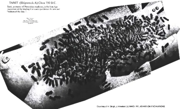
The Tanit shipwreck had 385 nearly identical amphoras exposed on the surface (see Figure 3-2). The only other types of artifacts that were visible were one stone anchor and several cooking pots [2]. There are three obvious questions that cannot be answered by the surface surveys and selected objects that were lifted. First, were there other types of cargo such as metal ingots. Second, is any of the hull preserved? And finally, what is the total size of the cargo? A precise sub-bottom profiler is in the unique position of potentially being able to answer these questions without excavating the wreck site.
The data that was collected (see Figure 3-1) is highly promising. It demonstrates that the profiler can detect some archaeological artifacts below the sea floor. Because the surface of the shipwreck has many exposed amphoras, the surface scattering conditions are complex. Because a pile of amphora is not a good boundary to couple the acoustic energy into the sea floor it is possible that much of the coherent energy is lost due to diffraction and scattering at this interface.
A zoomed in version of one shows several features below the sea floor (Figure 3-3.) The vaguely round orange objects in the surface layer are likely to be amphora. The
"ringing" effect noticed (left side) is likely to be reverberations of the sound wave inside an amphora situated in the ideal orientation [22]. The amphora average 69 cm in height and 22 cm in width which corresponds very well with the size of the observed objects. In addition there are several dark objects in the right hand side of the blown up image. The nature of these objects is unknown but it is likely that they are related to the shipwreck [22].
Although the images are highly promising, it is clear that there is room for im-provement. The images do not have the desired resolution nor do they provide as much information as possible about the objects buried beneath the surface. Without a quantitative understanding of how the sensor should respond to different types of buried objects, a positive identification of any target is impossible.
Figure 3-1: A vertical cross section taken by the prototype sub-bottom profiler of
the Tanit shipwreck (circa 750 BC) located in 400 meters of water off the coast of
Ashkelon, Israel
TANIT (Shipwreck A) Circa 750 B.C. Tat. PtoU Of the Secm. . 166WI Ow imwp: st 1IIP-uu f aIa ie 1 Iz, e;a fp1.%qc~e: As'afloIM
"Ashcra ofthc Sce "
Figure 3-2: Photomosaic of the Tanit shipwreck. Courtesy of H. Singh, J. Howland,
WHOI, IFE, and Ashkelon Excavations.
Figure 3-3: Expanded view of the cross-sectional imaged produced by the sub-bottom
profiler.
3.3
Monitor Turret Survey
The sensor was tuned up and a better time varying gain system was added before
the bottom profiler was used in a field experiment in North Carolina. The
sub-bottom profiler was carried by divers during a survey of the turret of the Monitor
off Cape Hatteras in the Summer of 2001
[3].
Unfortunately the amount of metal in
and around the turret of the Monitor proved to be a very hostile environment. Echos
due to side-lobe reflections and the complexity of the sub-surface returns obscure
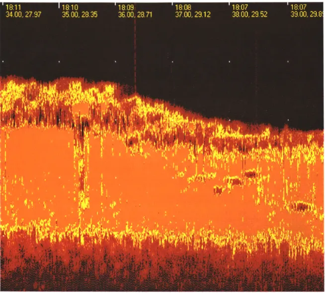
positive identification of possible buried objects (see Figure 3-4). The possible target indicated in the figure was recorded about 1 to 1.3 milliseconds after the first surface reflection. This corresponds to a depth of on the order of 1 meter.
Punctuation: divers raise and
lower xducer to signal start/end
a)
of survey line.
Sonar side lobe
reflection from armor belt
x Primary echo - first
return from
sediment
Second echo
bounce
b)
Echo from turret
walls Surface of sediment in turret - concave shape is excavation hole Layers or objects
Mort Within sediment
Hard target / buried
Ohiect
Figure 3-4: Sub-bottom profiler data from the survey of the exposed portion of the
Monitor turret is represented in the upper figure (a). The lower figure (b) is a close
up, with the x-axis representing survey time and the y-axis is acoustic travel time
in number of samples (500 samples
=
6.5 ms or about 5 meters.) Three distinct
echos indicate stratified sediment, or buried structure, and a distinct "hard" target is
evident. Figure and analysis courtesy of Brian Bingham, David Mindell and Brendan
Foley [3].
Chapter 4
Electronics and Signal Processing
in the Current System
In order to collect quantitative data with the sub-bottom profiler it is necessary to be able to correlate the numerical values recorded by the data logging system with voltage values from the transducer. Additionally in order to improve the system, it is necessary to carefully analyze the characteristics of the current system and look for possible sources of error and/or opportunities for improvement. The signal processing and data collection electronics are the logical place to begin this investigation because they are the easiest to examine in the laboratory and also the easiest to modify.
4.1
Overview
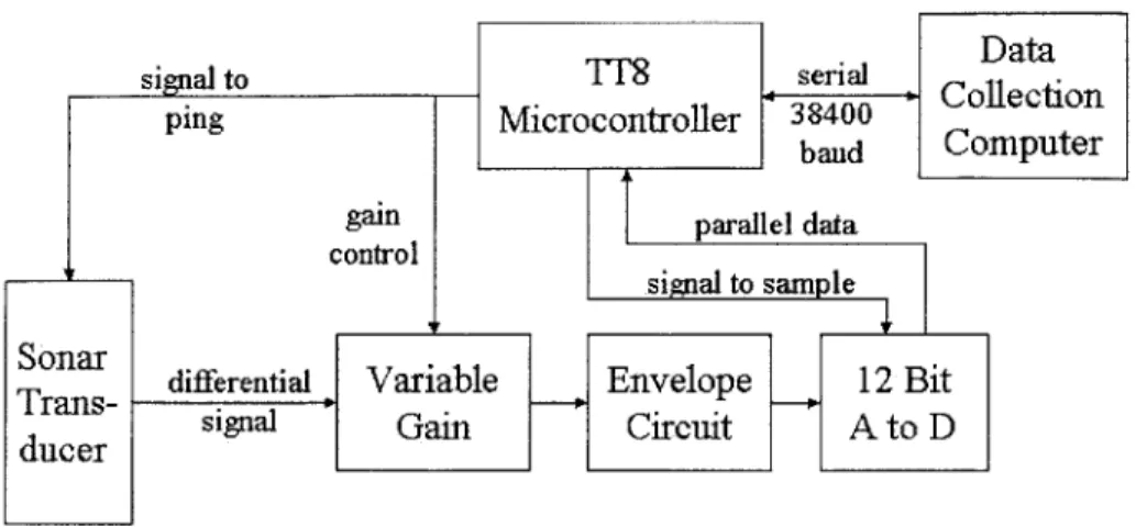
The data collection system amplifies, filters, digitizes, and logs the signal from the transducer. Consequently, the data collection system consists of 4 functional parts: time varying gain, enveloping, digitization and serial communication, and computer control. A block diagram of the system can be found in Figure 4-1. Schematics of the current electronics are located in Appendix A.
The laptop computer, located on the surface, has a real time display of the data as well as a convenient graphical interface for setting the number of samples, gain, and signal to start and stop collecting data. The computer program is responsible for
si alto
TF8
serial
Cata
ping Microcontroller ' 38400 Collection
baud Computer
Figure 4-1: Block diagram of the electronics
logging the data and sending control signals by serial cable down to the TattleTale 8 (TT8) microcontroller located on the vehicle near the sea floor.
The TT8 (indirectly) signals the transducer to ping by lowering the power supply voltage for 10 ,usec. The TT8 is also responsible for controlling the time varying gain system and signaling analog to digital converter to sample.
Time varying gain is accomplished by a combination of the TT8, a digital to analog converter and a variable gain amplifier. Indirectly by way of a digital to analog converter, the TT8 provides a 0 to 12 volt control signal to the variable gain amplifier. At constant intervals, the TT8 increases the gain according to predetermined values. Due to limitations in bandwidth to transmit data back to the surface and the limitations of the digital to analog converter, Mindell and his team decided to envelope the signal. The enveloping circuit rectifies the received signal and low-pass filters it to obtain the envelope of the pulse shape. The enveloped signal is passed to a 12-bit analog to digital converter which samples at about 80 kHz. The TT8 then passes the digitized data up to the computer on the surface for display and logging.
In an attempt to verify that the electronics have the desired behavior and to add to our knowledge of the system, I have performed several laboratory measurements as well as made numerical models of the systems.
4.2
Pulse Shape and Bandwidth
Since the transducer is sealed to operate at high pressures, I was unable to examine the electronics which generate transducer waveform nor was I able to examine the
pre-amp used in the receiver.
Marty Wilcox of Marine Sonics claims that the electronics produce a uniform 6 cycle pulse. The sonar signal output from a transducers is commonly a modified version of the electrical waveform. Marine Sonics claims that the transducers have a
Q
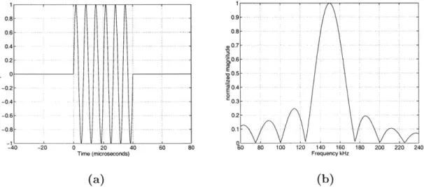
value and thus modify the pulse shape into a one which is slightly wider than a Gaussian pulse. Without measuring the properties of the transducer or the actual transmitted acoustic wave it is not possible to determine the exact shape. However, the resulting pulse shape is probably between the initial uniform or square-shape and a Gaussian.It is possible to calculate the frequency content of both the uniform pulse and the Gaussian pulse by Fourier transform. Figure 4-2 shows the uniform pulse shape in both the time and frequency domains. Similarly, Figure 4-3 is the Gaussian pulse in both time and frequency.
0.8 - -..--. 0.9 - -0.6 0.8 -0.4- 0.7 0.2- .6 -E O.5 E -0.2 - 0.4 -0.4- .0.3--0 .6 - - --- -- 0 .2 - - - --0.8 - 0.1--40 -20 0 m20 40 6O 80 60 80 100 120 140 160 180 200 220 240
Time (microseconds) Frequency kHz
(a)
(b)
Figure 4-2: The uniform pulse in the time domain (a) and the frequency domain (b).
It should be noted that the half power bandwidth of the Gaussian pulse, about 30 kHz, is considerably wider than the uniform pulse has a bandwidth of 23 kHz. However, if the two signals have and equal maximum amplitude in the time domain,
1 0.8 0.6 0.4 0.2 0 -0.2 -0.4 -0.6 -0.8 -40 -20 0 20 40 60 Time (microseconds) 0.9 0.8 ,0.7 0.6 -0.5 '0.4 0.3 0.2 0.1 80 '60 80 100 120 140 160 Frequency kHz 180 200 220 240
(a)
Figure 4-3: Gaussian pulse in the time domain (a) and the The magnitude in the frequency domain is normalized to the
the total power of the Gaussian the closer the actual signal is to resolution of the sensor, and the of penetration.
(b)
frequency domain (b). uniform pulse.
pulse is less than that of the uniform pulse. Thus, a Gaussian enveloped pulse, the greater the vertical closer it is to a uniform pulse, the greater the depth
4.3
Power Consumption
The current prototype electronics are rather inefficient in terms of power consumption. The electronics and an active transducer pinging once per second requires 11 Watts. The electronics alone without the transducer connected require 8.4 Watts. Thus, only 2.6 Watts or 24 percent of the total power could possibly be being used by the transducer. The system was designed to run off of a 12 Volt DC power supply, but the sonar transducer requires 48 Volts DC. Therefore it is likely that much of the power is wasted by the DC to DC converter. Since this prototype system was not designed for minimum power consumption this design choice is understandable.
- -. -. -. - -. -. ...-. -. - . .- .
-.... -... -.. - ... -..
- - - ---- -- - -- -- -.-- -.-- - --- .
Table 4.1: Power Consumption
Voltage Current Power
Electronics, no transducer 12 V 0.7 A 8.4 Watts
Electronics + Transducer silent 12 V 0.75 9 Watts
Electronics + Transducer pinging 1/sec 12 V 0.92 A 11 Watts
4.4
Time Varying Gain
The time varying gain system was designed to compensate for the rapid attenuation of pressure waves in sediment at high frequencies and the limited dynamic range of the analog to digital converter. In order to properly calibrate the system it is necessary to quantify the actual gain of the system as a function of time, that way the raw data can be reconstructed during post-processing. Without knowing the actual system gain as a function of time, the images that are created are limited to being pretty pictures and will never have quantitative meaning.
The attenuation in water is much less than it is in sediment, so it is desirable have the system gain increase at a constant rate after the first reflection from the sea floor is received. An approximation to the behavior was achieved as follows. The
TT8 receives a list of predetermined gain parameters provided by the user of the
system. The user can also specify a "lockout" number in microseconds corresponding to the approximate height the sensor is above the sea floor. By updating the gain parameter at constant intervals (400 psec) the gain can be increased over time. The gain parameter is a number ranging from 1 to 99.
The gain parameter is converted to an analog voltage value between 0 and 12 Volts. This conversion is linear in that if the numerical gain parameter in increased
by 1 the analog voltage level is increased by 0.12 Volts. This analog voltage is scaled
to 0 to 2.5 volts by a voltage divider and passed to the variable gain circuit designed
by Marty Wilcox of Marine Sonics. This variable gain circuit maps a linear change
in control voltage to a exponential change in amplification using an AD605.
each amplifier can provide between 0 and 48 dB of gain depending upon the input gain control voltage. For this application the two amplifiers were wired in series to give a total range of 0 to 96 dB. The amplification in decibels varies linearly with the input gain control voltage over the range from 8 to 88 dB. The amplifiers provide an additional 8 dB of gain on either side of this range, however it is not linear. The linear region corresponds to input gain control voltages of 0.5 to 2.5 Volts, or a numerical gain parameter between 20 to 100.
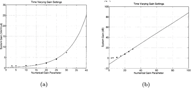
The behavior of the variable gain amplifier was tested by experimental measure-ments in the laboratory. The sonar receiver was replaced with a 150 kHz sine wave signal. The numerical gain parameter was varied and the ratio of output voltage to input voltage was calculated (see Figure 4-4.) Various input voltages were tested varying from 150 mV to 0.6 V. The experimental measurements agree very well with the expected behavior. All of the data points above a numerical gain parameter of 20 matched the predicted "ideal" values very well, whereas the those below 15 exhibit the non-linear behavior of the amplifier. In the region from 20 to 100, an increase in the numerical gain parameter of 1 corresponds to a 1 dB increase in gain.
30 Time Varying Gain Settings Time Varying Gain Settings
100 25- 80
~82O
CO20 - 60-0 E (n10 20-5-0~ O -20 -0 5 10 15 20 25 30 35 40 0 20 40 60 80 100Numerical Gain Parameter Numerical Gain Parameter
(a) (b)
Figure 4-4: The solid line is the predicted gain as a function numerical gain parameter. The asterisks are the experimentally measured values. The left figure (a) is the gain expressed as a ratio and the right figure (b) is the same data on a log scale expressed
in terms of decibels (20log10(Vut/Vjn)).
the variable gain circuit, it would be better to be operating in the linear region of the amplifier. Data collected during the survey of the Monitor turret indicates that this might not always be practical. A typical time varying gain parameter setting started at 10 and ended at 40 by increasing in steps of 2 about every 400 microseconds. However, it should be noted that the increase in amplification began before the primary return from the sediment, so the gain settings corresponding to sediment returns were mostly in the linear region.
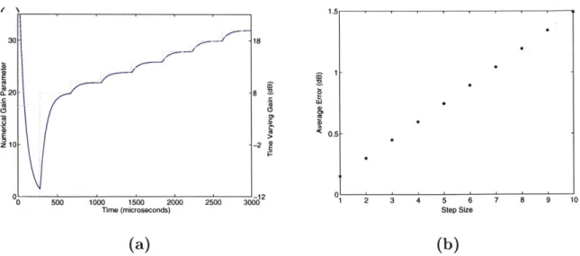
Laboratory measurements indicate that the actual time varying gain as a function of time is not quite as simple as an increase in gain parameter every 400 microseconds. The time between increases in gain is actually about 390 microseconds and there is a 280 microsecond delay after the ping but before the time varying gain settings begin. The system begins collecting data immediately. In addition to this built in delay in the time varying gain, the user can specify a lockout period in microseconds which corresponds to the height the sensor is position above the sea floor. The system delays the start of the time varying gain and does not collect any data during this period. Figure 4-5 (a) shows the effective numerical gain parameter as a function of time.
One other property of the variable gain circuit that is worth mentioning is that gain control voltage is passed through a low pass filter prior to being used by the variable gain amplifier. According to the schematic, this RC low-pass filter has a time constant of about 80 microseconds, which agrees well with laboratory observations. Consequently, as the gain is changed each "stair step" in amplification is effectively rounded off (see Figure 4-5 (b). ) Thus, no sharp lines are noticeable in the resulting image. While this filter improves the displayed image, it makes it difficult to calculate the exact system gain as a function of time.
There are two different ways that the system gain can be modeled as a function of time. The first and simplest method is to model the gain as a linear increase with time. The second method is to model the entire system by passing the ideal "stair-step" gain though a low-pass filter with a time constant of 80 microseconds. The second method is more accurate, but it is also more complicated.
4000 3500 40 - -28 3000-2500 30 - -18 C 0 2000 20 - 4 - - 8 1500 -Z 1000. 10 - - - -2 500
Time (milliseconds) Time (milliseconds)
(a)
(b)
Figure 4-5: Tine varying gain as a function of time for a gain setting which starts at
20 and increases in steps of 2. The left figure, (a), is the gain parameter as a function
of time. The right figure, (b), is the data collected by the system when the transducer
is replaced with a 150 kHz sine-wave that is 160 mV peak-to-peak in amplitude. The
dashed line is the modeled data.
fitting a line to the data. The best fist line has a slope of the step-size times 2.56
dB/ms and is delayed by 555 microseconds (i.e. 275 microseconds in addition to
the 280 microsecond delay discussed earlier.) This method is particularly poor at
approximating the gain in initial half a millisecond after data collection begins. The
equation of the best fit line is:
Gain[dB] = Start - 12 + Step * (2.56[dB/ms]) * (Time - 0.555[ms]) (4.1)
The amount of error caused by approximating the system gain as a linear increase
is dependent on the step size. The larger the step size, the more error is introduced.
The average amount of error for any given step size can be expressed as the square
root of the mean squared error. A graph of the average error for various step sizes
can be found in Figure 4-6 (b). For a step size of 2, the average error is about 0.34 dB
and the maximum error is 0.6 dB. Thus, the linear approximation is fairly accurate
for small step sizes, but is not very good for large step sizes.
30 - 18 20 -20 8 0.5 z10- -2 0 500 1000 1500 2000 2500 30 0 0 4 z6 7 8 9 10
Tim (microseconds) Step Size
![Table 3.1: Specifications for a prototype sub-bottom profiler from Mindell and Bing- Bing-ham, 2001 [22].](https://thumb-eu.123doks.com/thumbv2/123doknet/13955831.452591/30.918.250.670.265.486/table-specifications-prototype-sub-profiler-mindell-bing-bing.webp)