Publisher’s version / Version de l'éditeur:
Vous avez des questions? Nous pouvons vous aider. Pour communiquer directement avec un auteur, consultez la première page de la revue dans laquelle son article a été publié afin de trouver ses coordonnées. Si vous n’arrivez pas à les repérer, communiquez avec nous à [email protected].
Questions? Contact the NRC Publications Archive team at
[email protected]. If you wish to email the authors directly, please see the first page of the publication for their contact information.
https://publications-cnrc.canada.ca/fra/droits
L’accès à ce site Web et l’utilisation de son contenu sont assujettis aux conditions présentées dans le site LISEZ CES CONDITIONS ATTENTIVEMENT AVANT D’UTILISER CE SITE WEB.
8th International Conference on Short and Medium Span Bridges: 3 August 2010,
Niagara Falls, Ontario, Canada [Proceedings], pp. 106-1-106-10, 2010-08-03
READ THESE TERMS AND CONDITIONS CAREFULLY BEFORE USING THIS WEBSITE.
https://nrc-publications.canada.ca/eng/copyright
NRC Publications Archive Record / Notice des Archives des publications du CNRC : https://nrc-publications.canada.ca/eng/view/object/?id=edaf305e-0734-4b69-baf7-125268c38850 https://publications-cnrc.canada.ca/fra/voir/objet/?id=edaf305e-0734-4b69-baf7-125268c38850
NRC Publications Archive
Archives des publications du CNRC
This publication could be one of several versions: author’s original, accepted manuscript or the publisher’s version. / La version de cette publication peut être l’une des suivantes : la version prépublication de l’auteur, la version acceptée du manuscrit ou la version de l’éditeur.
Access and use of this website and the material on it are subject to the Terms and Conditions set forth at
Live load distribution on rigid frame concrete bridge
http://www.nrc-cnrc.gc.ca/irc
Live loa d dist ribut ion on rigid fra m e c onc re t e bridge
N R C C - 5 3 2 3 5
M e r g e l , P . ; A l m a n s o u r , H .
M a y 2 0 1 0
A version of this document is published in / Une version de ce document se trouve dans:
8th International Conference on Short and Medium Span Bridges, Niagara Falls,
Ontario, Canada, August 3-6, 2010, pp. 106-1-106-10
The material in this document is covered by the provisions of the Copyright Act, by Canadian laws, policies, regulations and international agreements. Such provisions serve to identify the information source and, in specific instances, to prohibit reproduction of materials without written permission. For more information visit http://laws.justice.gc.ca/en/showtdm/cs/C-42
Les renseignements dans ce document sont protégés par la Loi sur le droit d'auteur, par les lois, les politiques et les règlements du Canada et des accords internationaux. Ces dispositions permettent d'identifier la source de l'information et, dans certains cas, d'interdire la copie de documents sans permission écrite. Pour obtenir de plus amples renseignements : http://lois.justice.gc.ca/fr/showtdm/cs/C-42
Proceedings of 8th International Conference on Short and Medium Span Bridges
Niagara Falls, Canada 2010
106-1
LIVE LOAD DISTRIBUTION ON A RIGID FRAME CONCRETE BRIDGE
Patrick R. Mergel, M.Eng., P.Eng., ing. Delcan Corporation, Canada
Husham Hammadi Almansour, Ph.D.
Institute for Research in Construction, National Research Council Canada
ABSTRACT
Rigid frame concrete bridges were popularized in North America in the 1920s and 1930s as river crossings and highway grade separations. Short and medium span rigid frame bridges are still widely used today for rail/roadway grade separations in urban areas with constrained right-of-ways or with minimal vertical and/or horizontal clearances, as well as in rural areas due to the simplicity of their construction. Despite their popularity, there has been very little research on the live load distribution of current design vehicles on this type of bridge structures. The objective of this study is to examine the safety and accuracy of the existing load distribution method in the Canadian Highway Bridge Design Code (CHBDC), CAN/CSA-S6-06, using advanced modeling techniques. This study compared the analytical results of the live load distribution on a rigid frame concrete bridge, obtained using the Simplified Method of Analysis of the CHBDC with the results of a three dimensional finite element model (3D-FEM). For a 13 m clear span rigid frame bridge investigated in this study, the results show that the live load distribution values of the current CHBDC are 10% more conservative for longitudinal bending moments and approximately 15% more conservative for longitudinal vertical shears than the values obtained from the FEM analysis. Given the results of this study, and the limited previous investigations on this topic, further research on the live load distribution of rigid frame concrete bridges is required using a wide range of bridge spans, number of loaded lanes, boundary conditions, abutment wall width, material properties and slab thickness.
1. INTRODUCTION
German engineers were the first to pioneer the rigid frame or portal frame bridge, but it gained popularity in the United States in 1920s due to Westchester County, NY engineer Arthur G. Hayden (PCA, 1936). The new bridge type was developed for the Bronx River Parkway Reservation project, as a cost-effective and attractive alternative to the conventional arch bridge, which required massive abutments and significant excavation/grading to accommodate its relatively high profile.
The strength of a rigid frame concrete bridge originated from the rigid connection of the vertical abutment walls with the horizontal deck slab, resulting in a shallow midspan section. This bridge type had a unique ability to redistribute loads throughout the structure until it reached a balance, if any one element of the bridge was overstressed. Their immense strength and rigidity provided an additional safety in the structure. The result was a bridge that provided greater structural strength than reinforced concrete girder bridges. Engineers at Columbia University tested the new design and determined that the strength was nearly doubled what Arthur Hayden had originally calculated (HABS/HAER 2001).
Given the shallow midspan sections permitted by the innovative new rigid frame bridges, they were ideal for grade separation structures as their comparatively flat arch offered improved clearance over the well-defined curvature of traditional arch bridges, providing a minimum difference in the elevations between the roadway surfaces. With a more efficient profile reducing the overall height of the structure, rigid frame concrete bridges required less approach fill,
less excavation, and less concrete for the abutments and deck superstructure, which made their construction very appealing to highway departments throughout North America.
By the 1930s and 1940s, these structures became common for river crossings (Figure 1) and grade separations. Short and medium span rigid frame concrete bridges are still widely used today for rail/roadway grade separations in urban areas (Figure 2) with constrained right-of-ways or with minimal vertical and/or horizontal clearances.
Figure 1. Highway M-28 Sand River Bridge (1939), Alger County, Michigan (Photo: Courtesy of the Michigan Department of Transportation)
Figure 2. East Transitway Blair Road Underpass, Ottawa, Ontario (1989)
Typical rigid frame bridges consist of a haunched deck slab connected to abutment walls with adjoining wingwalls. The haunch of the deck slab is usually parabolic, although midspan sections of uniform thickness, which taper at either end to a deeper section at the abutment walls, are becoming more popular as they are simpler to construct. The back of the abutment walls are typically slanted and taper towards the footing. The wingwalls, used to retain the approach fill, are supported on the abutment footings.
The concrete abutments and deck of a rigid frame structure are cast-in-place, and occasionally poured monolithically, which results in walls that support the deck slabs as a continuous unit. The need for bearings is eliminated by the integration of the abutment wall and deck, providing a frame with rigid corners. This type of construction produces a very stable structure. The lower ends of the vertical members must resist the horizontal thrusts produced by the frame action of the structure; therefore, selection of this type of structure is preferred in locations where the foundations are very rigid.
In rigid frame structures, the interaction of the walls (or legs) and slab (or beams) generates positive and negative moments throughout the structure. Since all the members of a rigid frame bridge are working together as an integral
system, providing flexural resistance to support the superstructure, the moments and deflections are smaller near the center section of the deck compared to a bridge of the same span length simply supported on the abutments. The resulting effect is that the members and sections of the frame can be reduced to relatively slender proportions and therefore the bridge deck made significantly shallow at the midspan.
Although rigid frame concrete bridges have been constructed in North America since the 1920s, very few studies have examined the live load distribution due to moving vehicles. Hence, there is a need to investigate their behaviour in depth concerning the live load models, the design trucks, and the deflection/vibration limits in the current highway bridge design codes.
The objective of this study is to investigate the accuracy of the simplified method of analysis for live load distribution in the current Canadian Highway Bridge Design Code (CHBDC), CAN/CSA-S6-06 (CSA 2006), compared to a three dimensional finite element model. The study examined a single-span rigid frame concrete bridge with two lanes of traffic.
2. EXISTING RESEARCH & CURRENT BRIDGE CODE 2.1 Previous Studies of the Live Loading on Rigid Frame Bridges
Researchers in Virginia completed one of the first comprehensive studies on the live load distribution on frame bridges in the mid 1970s. They examined the live load on a frame bridge formed from five three-span welded steel rigid frames with two inclined I-shaped columns as interior supports and a concrete deck casted compositely to the steel frames. The stresses produced by loading the structure with the HS20-44 loading at five positions were measured and compared with (i) calculated stresses following the live load distribution method of AASHTO specifications; and (ii) calculated stresses using a 3-D finite element analysis model. The comparison indicated that the AASHTO specifications design guide for lateral load distribution to the stringers were very conservative (Kinnier and Barton 1975). The authors also observed that measured live load stresses were small compared to those results of the finite element model (Kinnier and Barton 1975). The study only looked at the effects of the live load when running one test vehicle across the deck at a time while it ignored the combined effects of multiple vehicles/lanes. In the 1970s, the Ministry of Transportation and Communications of Ontario (former MTO) conducted field tests on existing rigid frame bridges. These tests revealed that the stiffness of short-span portal frame bridges was greater than that predicted by conventional design procedures (Robbins and Green 1979). They investigated the static loading on a 1/24 plexiglass scale model of a prototype single span reinforced concrete with a haunched slab deck. Two types of static loading were considered: (i) a single point load placed at 6 locations on the deck; and (ii) a loading configuration to simulate a three-axle truck, or section of a tractor-trailer, placed at 5 locations on the deck. The experimentally measured stresses were compared to those stresses calculated using (i) simple beam theory; and (ii) finite element analysis. The results indicated that using the “effective width concept”, suggested by CSA S6-1974 for design, was conservative for portal frame bridges with varying depth (Robbins and Green 1979). The study concluded that simple beam theory, where the full width of the structure resists moment, can be more appropriate for strength evaluation for one of two loaded lanes (Robbins and Green 1979). The investigation was performed using static point loads and hence, the dynamic effect of moving vehicles was not considered. Huang, et al (1994) studied the vibration and impact effects of two trucks passing side by side on a slab-beam frame bridge (and not a solid frame bridge). The researchers carried out a dynamic finite element analysis on a frame bridge of almost the same general dimensions of the bridge in Kinnier and Barton’s study, but the interior support legs were not slanted. They use the live load model of AASHTO specifications, 1989, using the HS20-44 design truck. The design truck was modeled at various speeds using a nonlinear vehicle model. They found that the maximum impact factors in AASHTO specifications were higher than the impact factor from their model.
2.2 CHBDC Live Load Distribution Method
The Simplified Method of Analysis specified in Clause 5.7.1 of the current Canadian Highway Bridge Design Code (CHBDC), CAN/CSA-S6-06, allows a bridge to be treated as a beam for live load analysis. Rigid frame structures are categorized as “shallow superstructures”, as per Table 5.2 of the CHBDC; hence, a live load analysis requires determining the longitudinal bending moments due to live loads, as specified in Clause 5.7.1.2, as well as the longitudinal vertical shears due to live loads, as specified in Clause 5.7.1.4. The live load analysis, using the Simplified
Method of Analysis, or refined methods, requires determining the applicable loading on the structure. Clause 3.8 of the CHBDC specifies this loading as the CL-W loading, consisting of the CL-W Truck or CL-W Lane Load.
2.2.1 Longitudinal Live Load Bending Moment
For a bridge categorized as a shallow superstructure, the governing live load moments for ULS and SLS are determined by the method outlined in Clause 5.7.1.2.1.2, by treating the bridge as a beam for two load cases: (i) one CL-W Truck Load multiplied by the factor (1+DLA); and (ii) CL-W Lane Load. The governing live load moment of the two load cases per design lane is MT. For slab bridges (including rigid frames), the longitudinal moment, m is calculated per metre width:
[1] m = Fm*mavg
where Fm is the amplification factor to account for the transverse variation in maximum longitudinal moment intensity, as compared to the average longitudinal moment intensity and mavg is the average longitudinal moment per metre of width due to live load.
[2] Fm = B ≥ 1.05 F [1+ (μ*Cf)/100]
where B is the total width of bridge, F is the width dimension that characterizes the load distribution of a bridge, Cf is the percentage correction factor used to adjust the F value for longitudinal moment (F and Cf are obtained from Table 5.3 of the CHBDC), and μ is the lane width modification factor.
[3] μ = We -3.3 ≤ 1.0 0.6
where We is the width of design lane (Clause 3.8.2).
[4] mavg = n*MT*RL Be
where n is the number of design lanes (Clause 3.8.2), MT is the maximum moment per design lane at the point of the span under consideration, RL is the modification factor for multi-lane loading (Clause 3.8.4.2), and Be is the effective width of the bridge (reducing for tapered edges).
The calculation of the average moment intensity, mavg, accounts for the reduced probability of having more than one lane critically loaded at the same time, with the multi-lane loading reduction factor RL.
2.2.2 Longitudinal Live Load Vertical Shear
The governing live load shears for ULS and SLS are determined by the method outlined in Clause 5.7.1.4.1.2. The governing live load shear of the two load cases per design lane is VT. For slab bridges (including rigid frames), the longitudinal vertical shear, v, per metre width:
[5] v = Fv*vavg
where Fv is the amplification factor to account for the transverse variation in maximum longitudinal vertical shear intensity, as compared to the average longitudinal vertical shear intensity and vavg is the average shear per metre of width due to live load.
[6] Fv = B/F ≥ 1.05
where B is the total width of bridge and F is the width dimension that characterizes load distribution of a bridge (obtained from Table 5.7 of the CHBDC).
[7] vavg = n*VT*RL Be
where n is the number of design lanes, VT is the maximum shear per design lane at the point of the span under consideration, RL is the modification factor for multi-lane loading, and Be is the effective width of the bridge (reducing for tapered edges). As with the calculation of the longitudinal bending moments, the average shear intensity, vavg, Equation 7 accounts for the reduced probability of having more than one lane critically loaded at the same time, with the multi-lane loading reduction factor RL. As well, the actual intensity represented by the envelope of the maximum longitudinal vertical shear intensities across the width of the bridge is reflected by the multiplication of the amplification factor Fv.
3. 2-D FRAME ANALYSIS VS 3-D FINITE ELEMENT MODELING ANALYSIS 3.1 Model Frame Bridge Structure
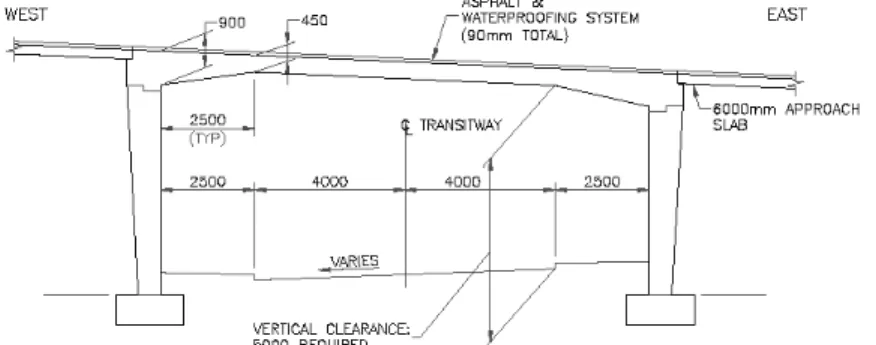
The model frame bridge structure used in this study consists of a single span reinforced concrete rigid frame bridge with a clear span length of 13m and the overall width of the structure is 13.75m. The cross-section includes the following elements (north to south): 2500mm concrete sidewalk (including a 300mm concrete parapet wall), 3750mm traffic lane, 3500mm traffic lane, 2000mm bicycle lane, and a 2000mm concrete sidewalk; a 300mm concrete parapet wall is also cantilevered on the exterior of the structure on the south side. Figure 3 shows a section of the structure from the south side, looking north and Figure 4 shows a typical cross-section of the structure from the west end, looking east. The back face of both abutment walls (or legs of the frame) is slanted from 900mm wide at the top to 600mm wide at the bottom. The deck has variable width haunches located at either end in order to facilitate the moment distribution at the top connection with the abutments walls. The structure is also located on a 4% superelevation; therefore, the height of the frame on the south side is higher than at the north side by approximately 550mm. As well, the bridge is located on a vertical grade of approximately 5.25%; therefore, the rigid frame structure has unequal legs, with the west abutment taller than the east abutment by approximately 600mm.
Figure 3. Typical section (south elevation) of the structure
Figure 4. Typical cross-section of the structure
3.2 2-D Frame Analysis (CHDBC Beam Analogy Method) 3.2.1 Analysis Approach
The standard design procedure for a rigid frame bridge is to reduce the applied loads and the structure to an equivalent unit width. Hence, the rigid frame concrete bridge is modeled as a 2-D rigid frame structure of unit-width elements with a structural analysis program using stiffness methods (including moment distribution method). The support conditions at the footings are assumed to be pinned. Due to the variable depth of the deck slab, the given cross-section was transformed by determining an equivalent area and depth of the deck.
X Y
Z
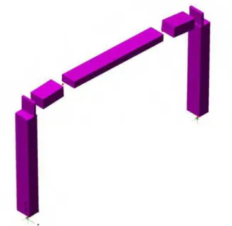
Figure 5. 2-D frame model of the rigid frame concrete bridge
3.2.2 Frame Model Description and Live Load Analysis
Based on the dimensions of the bridge shown in Figure 3, the structure was discretized into 10 elements. The nodes were located along the center of the members at the locations where the depth of the structure changes. The support conditions at the bottom of the legs are pinned, allowing only for rotation in the plane of the frame. As the width of the abutment walls and haunches vary over their length, the average width of the members was used in the model: 750mm for the abutments and 675mm for the haunches. Figure 5 shows a simple model of the 2-D rigid frame structure. The 2-D frame was created using linear elements of 1.0m width.
The live load analysis of the 2-D rigid frame structure was carried out by projecting the centreline of the CL-625-ONT design vehicle onto the deck of the structure (truck is centered over the 2-D frame) and moving the vehicle forward in increments of 0.50m. As the legs of the frame are unequal, the truck load is applied in both directions over the structure in order to capture the most critical effects. As the Lane Load rarely governs for structures with a span length less than 25m, its analysis was not considered in this study.
3.3 3-D Finite Element Model Analysis 3.3.1 Finite Element Model Description
A detailed 3-D finite element model of the entire rigid frame concrete bridge was developed using a commercial finite element structural analysis software. The model consists of “thick shell” elements, which allow for varying thicknesses along their length. In order to ensure the convergence and accuracy of the model analysis, three mesh refinements were examined. To confirm that the results of the modeling were converging to the optimum solution with increasing mesh refinements, the maximum moment/shear effects on the structure were compared.
X Y
Z
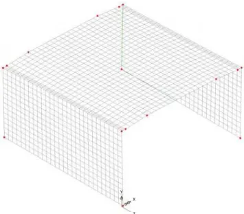
Figure 6. 3-D finite element model of the rigid frame concrete bridge
3.3.2 Live Load Analysis
The live load analysis of the 3-D rigid frame structure was carried out by projecting the centreline of the CL-625-ONT design vehicle onto the centreline of a single traffic lane (one lane at a time) on the deck of the structure and moving the vehicle forward in increments of 0.50m. As the frame legs are unequal, the truck load was applied in both directions (i.e. one truck in EBL and one truck in WBL) over the structure in order to capture the most critical effects.
4. ANALYSIS RESULTS AND DISCUSSIONS
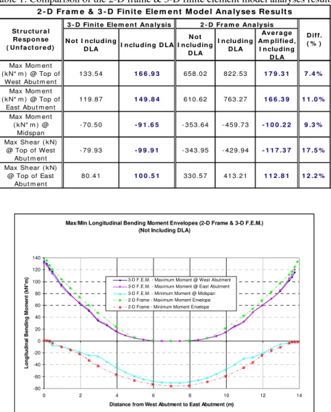
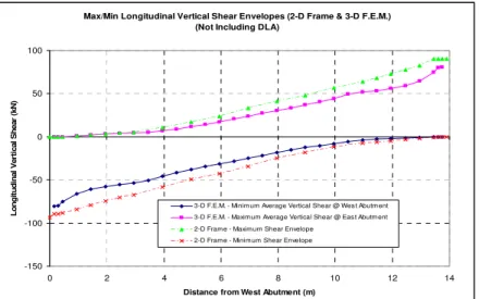
Following the live load analysis on the 2-D frame model, envelopes were created of the maximum/minimum longitudinal bending moment diagrams (Figure 7), as well as the maximum/minimum longitudinal vertical shear diagrams (Figure 8), for each position of the design vehicle in both traffic lanes. Examining the results of the 2-D frame model analysis, the maximum bending moment values (not including DLA) at the west abutment are approximately 8% higher than at the east abutment and the vertical shear is approximately 4% higher; therefore, it appears that the unequal legs only has a slight effect on the load distribution on the structure. The maximum
moment/shear due to the live loads obtained from the 2-D frame analysis are corrected to include the DLA (averaged and then amplified), as indicated in Sections 2.2.1 and 2.2.2, and the results are presented in Table 1.
Table 1 shows that: (i) the maximum longitudinal bending moments of the 2-D frame analysis are approximately 7-11% higher than that of the FEM; and (ii) the maximum longitudinal vertical shear of the 2-D frame analysis are approximately 12-17% higher than that of the FEM. The transverse variation of the longitudinal bending moment along the west and east abutments, as well as across the deck at the center of the span for the 3-D FEM are shown in Figure 9. The maximum moment at the west abutment occurs at approximately 4.9m from the north side of the structure, and the maximum moment at the east abutment occurs about 6.4m from the north side of the structure, or about at center of both traffic lanes located at 6.2m from the north end. The maximum moment at the centreline of the span occurs at about 5.4m from the north side of the structure. The transverse variation of the longitudinal vertical shear plotted for the 3-D FEM along both abutments (Figure 10) reveals sharp spikes at the locations of the wheel paths. These localized sharp increases in shear are most likely due to punching shear effects caused by the design vehicle wheel loads applied to finite element model, as they were idealized as discrete point loads.
The comparison of the live load longitudinal bending moment and longitudinal vertical shear results obtained from 2-D frame analysis with those obtained from 3-D FEM proves that the using the Simplified Method of Analysis
gives conservative estimation. This may be attributed to added stiffness provided by the deck slab of the rigid frame in resisting the applied live loading.
It was evident that the largest influences of the truck axles on the live load distribution originate from either a combination of Axles 1 to 4 or Axles 2 to 4 for the 2-D frame analysis. These findings correlate well with the 3-D FEM, where the largest influences on the live load distribution are from Axles 1 to 3 or Axles 2 to 4.
The longitudinal bending moment and shear diagrams (Figures 7 and 8) appear to correlate fairly well, but the values closer to the supports seem to have a greater difference between each other, producing more conservative results for the 2-D frame analysis. A possible explanation for this result could be that the average thickness of the haunches was used for the members for the 2-D frame analysis, but was accurately modeled for the 3-D finite element analysis; therefore, the distribution of the live loading across the haunches differs slightly due to differences in the stiffness of the members.
The effect of the bridge span length, the frame bridge type (solid or slab on rigid frames), and the materials properties on safety and accuracy of the CHBDC load distribution method are not investigated. It is apparent that there is a need to evaluate the limitation of the CHBDC live load distribution method for frame bridges.
Table 1: Comparison of the 2-D frame & 3-D finite element model analyses results
N ot I n clu din g D LA I n clu din g D LA N ot I n clu din g D LA I n clu din g D LA Av e r a ge Am plifie d, I n clu d in g D LA Max Mom ent
( k N* m ) @ Top of West Abut m ent
13 3.54 1 6 6 .9 3 658.0 2 82 2.53 1 7 9 .3 1 7 .4 % Max Mom ent
( k N* m ) @ Top of East Abut m en t
11 9.87 1 4 9 .8 4 610.6 2 76 3.27 1 6 6 .3 9 1 1 .0 %
Max Mom ent ( k N* m ) @ Midspan - 70.50 - 9 1 .6 5 - 353.64 - 459.7 3 - 1 0 0 .2 2 9 .3 % Max Shear ( kN) @ Top of West Abut m ent - 79.93 - 9 9 .9 1 - 343.95 - 429.9 4 - 1 1 7 .3 7 1 7 .5 % Max Shear ( kN) @ Top of East Abut m ent 80.41 1 0 0 .5 1 330.5 7 41 3.21 1 1 2 .8 1 1 2 .2 % 2 - D Fr a m e & 3 - D Fin it e Ele m e n t M ode l An a ly se s Re su lt s
3 - D Fin it e Ele m e n t An a ly sis St r u ct u r a l Re spon se ( Un f a ct or e d) 2 - D Fr a m e An a ly sis D iff. ( % )
Max/Min Longitudinal Bending Moment Envelopes (2-D Frame & 3-D F.E.M.) (Not Including DLA)
-80 -60 -40 -20 0 20 40 60 80 100 120 140 0 2 4 6 8 10 12 14
Distance from West Abutment to East Abutment (m)
Lo ng it ud ina l B e n d ing M o m e nt ( k N *m
) 3-D F.E.M. - Maximum Moment @ West Abutment
3-D F.E.M. - Maximum Moment @ East Abutment 3-D F.E.M. - Minimum Moment @ Midspan 2-D Frame - Maximum Moment Envelope 2-D Frame - Minimum Moment Envelope
Figure 7. Max/min longitudinal bending moment envelopes (2-D frame & 3-D F.E.M.) 106-8
Max/Min Longitudinal Vertical Shear Envelopes (2-D Frame & 3-D F.E.M.) (Not Including DLA)
-150 -100 -50 0 50 100 0 2 4 6 8 10 12 14
Distance from West Abutment (m)
L o n g it u d in a l V e rt ic a l S h e a r ( k N )
3-D F.E.M. - Minim um Average Vertical Shear @ West Abutm ent 3-D F.E.M. - Maximum Average Vertical Shear @ Eas t Abutm ent 2-D Frame - Maximum Shear Envelope
2-D Frame - Minimum Shear Envelope
Figure 8. Max/min longitudinal vertical shear envelopes (2-D frame & 3-D F.E.M.)
Transverse Variation of Longitudinal Bending Moment (3-D F.E.M.) (Not Including DLA)
-80 -60 -40 -20 0 20 40 60 80 100 120 140 0 2 4 6 8 10 12 1
Distance from North End (m)
Lo ngi tu di nal B e ndi ng M om e nt ( k N *m ) 4 Longitudinal Moment Along West Abutment
Longitudinal Moment Along East Abutment Longitudinal Moment Across CL of Span
Figure 9. Transverse variation of live load longitudinal bending moment (3-D F.E.M.)
Transverse Variation of Longitudinal Vertical Shear (3-D F.E.M.) (Not Including DLA)
-150 -100 -50 0 50 100 150 0 2 4 6 8 10 12 14
Distance from North End (m)
Longi tudi nal Ver ti cal S he a r ( k N)
Longitudinal Vertical Shear Along Wes t Abutm ent Longitudinal Vertical Shear Along East Abutment
Figure 10. Transverse variation of live load longitudinal vertical shear (3-D F.E.M.) 106-9
106-10 5. CONCLUSIONS
This study confirms that the Simplified Method of Analysis of the CHBDC (CAN/CSA-S6-06) leads to 7-17% higher estimation for the longitudinal live load bending moment and shear when compared to the results obtained of a three dimensional finite element model.
In order to understand the localized punching shear effects on the deck slab that was revealed by the finite element analysis, further study is required. As well, additional research is needed on the live load distribution of more than 2 design lanes and to investigate the effect of varying the span length, material properties and thickness of the deck on the live load distribution on rigid frame concrete bridges. The safety, the accuracy and the applicability limits of the CHBDC live load distribution method for rigid frame bridges are to be investigated in future research.
6. ACKNOWLEDGEMENTS
The assistance of the University of Ottawa’s Interlibrary Loans staff is gratefully acknowledged in locating some of the research material used in this paper. The Michigan Department of Transportation has also granted their permission for the use of a photo in this paper. The first author also acknowledges the patience and understanding of his wife, Annie, throughout the time spent on the research for this study.
7. REFERENCES
Canadian Standards Association. 2006. CAN/CSA-S6-06, Canadian Highway Bridge Design Code, Canadian Standards Association, Mississauga, ON, Canada.
Canadian Standards Association. 2006. S6.1-06, Commentary on CAN/CSA-S6-06, Canadian Highway Bridge Design Code, Canadian Standards Association, Mississauga, ON, Canada.
Hayden, A. G. and Barron, M. 1950. The Rigid-Frame Bridge, 3rd Ed., John Wiley & Sons, New York, NY, USA. Historic American Building Survey/Historic American Engineering Record (HABS/HAER). 2001. Bronx River
Parkway Reservation Report (HAER No. NY-327). Historic American Engineering Record, Westchester County, NY, USA.
Huang, D., Wang, T.-L., and Shahawy, M. 1994. Dynamic Loading of Rigid Frame Bridge, Structures Congress XII, American Society of Civil Engineers, Atlanta, Georgia, USA, 1: 85-90.
Kinnier, H. L. and Barton, F. W. 1975. A Study of a Rigid Frame Highway Bridge in Virginia (VHTRC 75-R47), Virginia Highway and Transportation Council, Charlottesville, Virginia, USA.
P.A.C. Spero & Company and Louis Berger & Associates. 1995. Historic Highway Bridges in Maryland (1631-1960): Historic Context Report, Maryland State Highway Administration, Maryland Department of Transportation, Baltimore, Maryland, USA.
Parsons Brinckerhoff Quade & Douglas Inc. 1997. Small Structures on Maryland’s Roadways: Historic Context Report, Maryland State Highway Administration, Maryland Department of Transportation, Baltimore, Maryland, USA.
Portland Cement Association. 1936. Analysis of Rigid Frame Concrete Bridges (Without Higher Mathematics), Fourth Edition, Portland Cement Association, Chicago, IL, USA.
Robbins, S. T. and Green, R. 1979. Portal Frame Bridge Behaviour, 1979 Annual Conference: Design Technical Session and Workshops, Roads and Transportation Association of Canada, Regina, Saskatchewan, Canada, D79-D100.