Algorithms for FFT Beamforming Radio Interferometers
The MIT Faculty has made this article openly available.
Please share
how this access benefits you. Your story matters.
Citation
Masui, Kiyoshi W. et al., "Algorithms for FFT Beamforming Radio
Interferometers." Astrophysical Journal 879, 1 (July 2019): 16 ©2019
Authors
As Published
https://dx.doi.org/10.3847/1538-4357/AB229E
Publisher
American Astronomical Society
Version
Final published version
Citable link
https://hdl.handle.net/1721.1/129686
Terms of Use
Article is made available in accordance with the publisher's
policy and may be subject to US copyright law. Please refer to the
publisher's site for terms of use.
Algorithms for FFT Beamforming Radio Interferometers
Kiyoshi W. Masui1,2 , J. Richard Shaw3, Cherry Ng4, Kendrick M. Smith5, Keith Vanderlinde4,6, and Adiv Paradise6 1
MIT Kavli Institute for Astrophysics and Space Research, Massachusetts Institute of Technology, 77 Massachusetts Avenue, Cambridge, MA 02139, USA;
2
Department of Physics, Massachusetts Institute of Technology, 77 Massachusetts Avenue, Cambridge, MA 02139, USA
3
Department of Physics and Astronomy, University of British Columbia, 6224 Agricultural Road, Vancouver, BC V6T 1Z1, Canada
4
Dunlap Institute, University of Toronto, 50 St. George Street, Toronto, ON M5S 3H4, Canada
5
Perimeter Institute for Theoretical Physics, Waterloo, ON N2L 2Y5, Canada
6
Department of Astronomy and Astrophysics, University of Toronto, 50 St. George Street, Toronto, ON M5S 3H4, Canada Received 2017 October 23; revised 2019 May 15; accepted 2019 May 16; published 2019 June 28
Abstract
Radio interferometers consisting of identical antennas arranged on a regular lattice permit fast Fourier transform beamforming, which reduces the correlation cost from ( )n2 in the number of antennas to (nlogn). We develop
a formalism for describing this process and apply this formalism to derive a number of algorithms with a range of observational applications. These include algorithms for forming arbitrarily pointed tied-array beams from the regularly spaced Fourier transform–formed beams, sculpting the beams to suppress sidelobes while only losing percent-level sensitivity, and optimally estimating the position of a detected source from its observed brightness in the set of beams. We also discuss the effect that correlations in the visibility-space noise, due to cross talk and sky contributions, have on the optimality of Fourier transform beamforming, showing that it does not strictly preserve the sky information of the n2correlation, even for an idealized array. Our results have applications to a number of upcoming interferometers, in particular the Canadian Hydrogen Intensity Mapping Experiment–Fast Radio Burst (CHIME/FRB) project.
Key words: instrumentation: interferometers– methods: observational – techniques: interferometric
1. Introduction
Interferometry has been central to the field of radio astronomy for 70 yr. Interferometers combine the signals from multiple antennas coherently to both increase sensitivity and gain spatial information. Many of today’s most successful radio observatories are interferometers with many dozen antennas.
In the past, the size of interferometers has been limited by the cost of the electronics that instrument the antennas and the computational cost to combine their signals. However, the latter has become less challenging with Moore’s Law, and the former has become dramatically cheaper with the advent of mass-produced electronics designed for the communications industry. This has permitted a new class of radio telescope composed of a large number—hundreds to thousands—of low-cost, typically nonsteerable antennas. These include the Canadian Hydrogen Intensity Mapping Experiment (CHIME7; Bandura et al. 2014), HERA8 (DeBoer et al. 2017), HIRAX
(Newburgh et al. 2016), LEDA9 (Greenhill et al.2012; Price et al. 2018), LOFAR10 (van Haarlem et al. 2013), MITEoR
(Zheng et al.2014), MWA11(Lonsdale et al. 2009), the Ooty
Radio Telescope (Saiyad Ali & Bharadwaj2013), PAPER12, Tianlai13(Chen 2012), and UTMOST14 (Caleb et al.2016).
Further scaling of this type of instrument is limited by the computational cost to pairwise correlate the antenna signals, which scales as n2in the number of antennas compared to n for
the mechanical and analog components of the telescope. As such, beyond a certain number of antennas, the telescope cost will once again be dominated by the computational correlation cost, even while the cost of computation is dropping over time. An alternate form of correlation was used on the Waseda Radio Telescope(Nakajima et al.1992; Otobe et al.1994; Daishido et al.2000) using a fast Fourier transform (FFT) of the antenna
signals in the spatial (antenna position) direction rather than pairwise correlation. The output of this process is localized beams on the sky rather than visibilities. In Pen(2004), it was
suggested that this method could be used for very large interferometers to reduce the correlation cost to scale as nlog ,n an idea that was formalized and extended in Tegmark & Zaldarriaga (2009, 2010) and implemented on the BEST-2
array by Foster et al.(2014). The concept was further extended
to apply to irregular and heterogeneous arrays of antennas by Morales (2011), which was extended and implemented in
Beardsley et al. (2017) and Thyagarajan et al. (2017).
Beamforming with FFT dramatically reduces the correlation cost, which in principle should allow for the construction of telescopes with many more antennas that will be orders of magnitude more sensitive than current instruments. It is envisaged that such telescopes will permit neutral hydrogen gas to be mapped over large volumes of the high-redshift universe, spurring a revolution in observational cosmology (Loeb & Zaldarriaga 2004; Furlanetto et al. 2006; Masui & Pen2010; Morales2011).
In the near term, FFT beamforming will be used at the CHIME (specifically CHIME/Fast Radio Burst (FRB); Ng et al. 2017; CHIME/FRB Collaboration et al. 2018) and
HIRAX telescopes to correlate roughly 2000 antenna signals and search for fast radio bursts. In this application, the calibration challenges that currently prevent FFT beamforming from being used for hydrogen surveys(Liu et al.2009,2010; © 2019. The American Astronomical Society. All rights reserved.
7 https://chime-experiment.ca 8 http://reionization.org 9 http://www.tauceti.caltech.edu/leda 10http://lofar.org 11 http://mwatelescope.org 12 http://eor.berkeley.edu 13http://tianlai.bao.ac.cn 14 https://astronomy.swin.edu.au/research/utmost
Newburgh et al.2014) are less severe. In hydrogen surveys, the
foregrounds are several orders of magnitude brighter than the signal, so small calibration errors can lead to a small fraction of the foregrounds leaking into the signal channel, which then swamps the signal. When using FFT beamforming, calibration must be performed in real time, whereas in traditional correlation, it can be done in offline analysis, allowing for a more careful calibration. On the other hand, FRBs are separated from contaminants in the time domain, and as such, the main concern is the sensitivity of the telescope to sky signals. We will discuss the effect of calibration errors in more detail in Section 3.4.
The use of FFT beamforming in FRB searches does present other challenges, however. The simplest FFT beamforming algorithms give little control over the locations of the beams on the sky, and these locations are wavelength-dependent. Transient surveys typically need to maximize instantaneous broadband sensitivity to a single location, rather than form a map of the static sky. As such, the chromaticity of the beam locations must be dealt with in some way, but the simplest methods of doing so introduce severe spectral structure in the beam shape (Ng et al. 2017). Another issue is a poor
understanding of the noise properties of individual beams and how it is correlated between them. This has led to confusion as to how well a transient source can be localized from a multibeam detection and the optimal algorithm for doing so.
In this article, we develop a formalism for beamforming, particularly focusing on FFT beamforming. We use this to address the issues discussed above and derive a number of algorithms with a range of observational applications. To orient the reader, the highlights of our work are summarized as follows. The formed beam that optimizes its response to a single point on the sky is given in Equation (30) or (32),
depending on the generality of the noise model assumed. In Section3.2we show that, for redundant arrays, using an FFT to form2nant-1beams has the same information content as the visibilities, but only if simplifying assumptions are made about the noise. For forming a large number of beams(for example, “fan beams” to perform blind searches for sources), Equation (50) allows the FFT beams to be exactly regridded
to arbitrary (and achromatic) positions using down-sampled intensities. Section4.1describes how a form of windowing can be used to suppress sidelobes, decrease the regridding cost, and increase the beam solid angle while losing only a small amount of peak sensitivity. This results in a net higher discovery rate in blind searches when the number of beams that can be searched isfixed. In Section4.3we derive the optimal estimator for the location of a source from a multibeam detection. In a follow-up work, we will use the strategies described here to perform a comprehensive optimization for upcoming experiments like CHIME/FRB.
2. Preliminaries
In this section, we will introduce our notation and conventions for describing the sky and instrument response. Our notation is based on that developed in Shaw et al. (2014,2015), although the underlying derivations are presented
in many other works(van Cittert1934; Zernike1938; Hamaker et al.1996; Smirnov2011; Thompson et al.2017). One source
of complexity in this work is the large number of different types of indices used to iterate over different spaces. For clarity, we summarize these in Table1.
2.1. Sky
An antenna samples the electricfield in a weighted volume surrounding its location. In detail, this response is complicated, as in the near field, the antenna itself serves to modify the electricfield. However, in our case, we only need the far-field response. To start, we write the electricfield in the absence of the antenna as the sum of plane waves coming from the far field,
ò
e n n = - pn -( ) ( ) ( ˆ ) ˆ ( ) ( · ˆ ) E x t n n c e d d , 1 , i t x n c , 1 0 2 2 1 2which defines the quantity e( ˆn,n). Here ˆn is a unit vector
defining a direction on the sky, andd2nˆis the differential solid angle. That the electricfield is real setse( ˆn,n)=e( ˆn,-n)*. We are generally not interested in the actual phase of the incoming electric field but are more concerned with its correlations áej( ˆn,n e) ( ˆ*k n¢,n¢ ñ). The index j runs over the polarizations of the incoming electricfield, which is described in terms of an orthogonal basis on the sphere. In this work, we will use the conventional decomposition along a basis in fˆ and
qˆ. In most cases, we can treat the emission as incoherent and
originating in the far field such that it is described by an intensity matrix * e n e n d d n n n n á ( ˆ ) ( ˆ¢ ¢ ñ =) ( ˆ - ¢ˆ ) ( - ¢) ( ˆ ) ( ) n n n n k n c I , , , , 2 j k B jk 2 2 2
which we express as a brightness temperature. Note that since
ò
d2( ˆ)n d2nˆ =1, the units of d2( ˆ)n are inverse steradians. Theabove equation can be decomposed in terms of Stokes parameters I, Q, U, and V, giving
= + + + ( ˆ)n ( ˆ)n ( ˆ)n ( ˆ)n ( ˆ)n ( ) Ijk IjkI jkQ U V , 3 Q jk U jk V
where the polarization matrices P are equal to the Pauli matrices in an orthonormal basis:
= = -= =
-( )
(
)
( )
(
i)
( ) i 1 0 0 1 , 1 0 0 1 , 0 1 1 0 , 0 0 . 4 jk I jk Q jk U jk V Table 1Indices Used, Their Meaning, and Implied Summation Limits unless Otherwise Given
Symbol Quantity Indexed Range
j, k , l, m Directions perpendicular to incident radiation
0 to 1 P The Stokes parameters (I Q U V, , , )
a, b, c, d Antennas 0 tonant-1 δ Difference between two feed
indicesa-b
-(nant-1)tonant-1
α “Redundancy” index com-plementary toδ
d
-( )
max 0,
tomin(nant,nant-d) A, B, C, D FFT-formed beams 0 toM-1
X, Y Label for beams within a generic set
For notational convenience, we will rewrite Equation(3) as
=
( ˆ)n ( ˆ)n ( )
Ijk PjkIP , 5
where there is an implied summation over the polarization index P, which we use throughout for repeated indices with one raised and one lowered. We thus have
* e n e n d d n n n á ( ˆ ) ( ˆ¢ ¢ ñ =) ( ˆ - ¢ˆ ) ( - ¢) ( ˆ) ( ) n n n n k n c I , , . 6 j k B jk P P 2 2 2
The strength of a single unresolved source at location ns is parameterized by its spectralflux density Fν, the power per unit collecting area per unit frequency(usually quoted in Janskys). This is related to the intensity I as follows. First, a short electricity and magnetismcalculation gives the flux per observed solid angle due to intensity vector IP:
n d n n n W= = n ( ˆ ) ( ˆ ) ( ) n n dF d k c I k c I , 2 , . 7 B jk jk P P s B s 2 2 2 2
From this, we can read off the unpolarized intensity associated with a single source(which we indicate with a superscript s):
n d n d n = -= - ´ n n - ⎜⎛ ⎟ -⎝ ⎞ ⎠ ⎛ ⎝ ⎜ ⎞⎠⎟ ( ) ( ˆ ˆ ) ( ˆ ˆ )( ) ( ) n n n n n I c k F F , 2 3.26 10 K 1 GHz 1 Jy . 8 s s B s 2 2 2 2 5 2
The way we have distributed the factors of 2 is such that for an unpolarized signal, the brightness temperature in a single polarization, say Ixx, has the same value as the unpolarized
intensity I. However, the flux density in a single polarization has half the value of the total flux. That is, the unpolarized brightness is the average of the brightnesses in the individual polarization components, whereas the flux is the sum of the flux of the polarization components.
2.2. Antennas and Visibilities
The signal at an antenna (normally measured as a digitized voltage) can be written in terms of these plane waves and an antenna response function Aja( ˆn,n)given by
ò
h = A ( ˆn,n e) ( ˆn,n)e pu n· ˆd nˆ +n ( )n , ( )9
a aj j i2 a 2 a
whereua =xa l, the feed position given in wavelengths, and n
( )
ni is the receiver noise. The antenna response,Aai( ˆn,n), is a complex 2D vectorfield giving the response to waves of both polarizations at every location on the sky. The response is normalized such that
*
ò
djkAaj( ˆn,n)Aak( ˆn,n) d2nˆ =1. (10) Note that in other works, the response is often normalized suchthat its maximum value is unity. The quantity
* d º ( ˆ)n
D jkA Aaj ak is the directivity (IEEE 2014), which is related to the effective area of the antenna by15Aeff =l2D. For a well-designed antenna, the effective area is related to the physical area of the antenna by an efficiency factor of order unity. The effective solid angle over which the antenna has response—or the beam solid angle—is thusW ~A l2 Aeff.
Antennas are often deployed in pairs with a complementary polarization response. That is, for each antenna, there is a second colocated antenna with a response that has a similar angular and frequency dependence but nearly orthogonal dependence in polarization space (index i). We treat these as distinct antennas with different a indices.
The quantity recorded by most radio interferometers is the visibility, the correlation between a pair of feeds. This is evaluated by estimating the covariance between feeds over a set of time samples, *
å
n h h º [ ] [ ] ( ) V c k n t t 1 , 11 ab B t a b 2 2 samp º á ñ = + ( ) Cab Vab Sab N ,ab 12where h [ ]a t are discrete time samples of the antenna signals ha, and the total number of samples we are averaging is
n º D D
nsamp t samples in time. In the second line, we have separated the expected visibility into contributions from the sky Sab and receiver noise Nab= án na b*ñ. Combining with Equations(6) and (9), we can express the measured visibility as
^ ^ ^ ^ ^
ò
n = n n * n p ( ) (n ) (n ) (n ) · n ( ) S A , A , P I , e u nd , 13 ab aj bk jkP P i2 ab 2whereuab =ua -ubis the vector separation between the feeds in wavelengths. With these definitions, if the sky is unpolarized and isotropic with brightness temperature T(i.e.,I(n,n =) T), then the sky autocorrelation isSaa=T.
In the case where the sky contains a single unpolarized point source, we can combine the above with Equation(8) to obtain
* n n d n n = n p ( ) ( ˆn ) ( ˆn ) · ˆ ( ) S c k F A A e 2 , , . 14 u n abs B jk aj s bk s i 2 2 2 ab s
This yields the notion of the antenna forward gain, the maximum response of the antenna to a point sourceSaas =G Ff n with Gf =c2djkA Aaj ak* 2kBn2=Aeff 2kB, which has units K Jy−1.
In many cases, we will adopt a simple noise model where receiver noise is constant, uncorrelated from antenna to antenna, and dominates over the sky:
n = n d ( ) ( ) ( ) ( ) N T T S simple noise , 15 ab ab ab r r
where Tr is the receiver noise temperature. However, most
results will be presented in as general a form as possible to facilitate extensions.
15
We will assume a calibration relative to a sky source and, as such, ignore losses parameterized by the radiation efficiency that would normally enter this equation. These losses instead get absorbed into the definitions of the noise properties(i.e., Tr, defined below).
The covariance of the visibilities is (Kulkarni 1989; Masui et al.2015) * n = D D (V V ) C C ( ) t Cov ab, cd ac bd. 16
This is convenient, since it often suffices to use Vab as an
estimate of Cabin the above formula, permitting the covariance
to be calculated directly from the data. Such a scheme is valid even if the visibilities are uncorrelated. A special case of the above equation is the variance of an autocorrelation ( = = =a b c d), where the equation reduces to
n = á ñ D D (V ) V ( ) t Var aa . 17 aa 2
In the case where the receiver noise dominates over the sky and is described by the simple system temperature model above, Equation(16) reduces to the familiar radiometer equation:
d d n = D D (V V ) T ( ) ( ) t
Cov ab, cd ac bd r simple noise . 18
2
3. Beamforming
We will define a beamformed visibility16 as any linear combination of the visibilities,
= ( )
b w V ,ab 19
ab
where we have defined the visibility space beamforming weights wab. We choose the beams to be normalized such that
*
å
w w =1. (20)ab ab ab
We will see in a moment that in the simple noise model, this normalization gives the beams the same variance as the visibilities. The beam’s expectation value in terms of the sky and noise is
ò
n n n áb( )ñ = Bjk( ˆn, ) I ( ˆn, )d nˆ +w N , (21) jk P P 2 ab abwith the beam response function(or beam shape function) * n = n n p ( ˆn ) ( ˆn ) ( ˆn ) · ˆ ( ) Bjk , w Aab , A , e u n. 22 a i b j i2 ab
The covariance of two formed beams is
* * n º = D D ( ) ( ) b b w C C w t Cov , , 23 XY X Y X ab ac bd Y cd
which, in the case of the simple noise model, is *
å
n = D D ( ) ( ) T w w t simple noise . 24 XY r2 ab Xab YabA special class of beams can be formed pre-correlation on the antenna signals, which can then be squared and integrated. These are termed factorizable beams, since their defining
feature is that, in visibility space, the beam weights factorize:
* *
å
å
n h n h h = = ∣ [ ]∣ [ ] [ ] ( ) b c k n w t c k n w t w t 1 1 . 25 f B t f a a B t f a a b b 2 2 samp 2 2 2 sampHence, for factorizable beams, we have * = ( ) wf w w . 26 ab f a f b
Since factorizable beams are the magnitude square of a linear combination of the pre-correlation antenna signals, they are strictly positive and have no negative lobes. In analogy to Equation(17), factorizable beams have the property that
n = á ñ D D ( )b b ( ) t Var f . 27 f 2
Note that the individual antenna patterns Aai have been normalized such that their intensity response integrates over angles to unity (Equation (10)). There is no such relation for
formed beams, where d Bjk jk may integrate to a quantity either less than or greater than unity. Our formalism is general enough to, for instance, describe beams that are the difference of two redundant visibilities, which would have no sky response. One case where the sky response does integrate to unity is for factorizable beams when the antenna responses are isotropic.
Throughout this article, several classes of beams are discussed, using different choices of the weights to achieve different goals. To orient the reader, we summarize these in Table2.
3.1. Pointed Beams
When studying discrete, unresolved, unpolarized sources on the sky, one often wants to maximize the response of the array to a single point at steering angle ˆnp. Such a beam signal weights the visibilities (based on Equation (14), setting ˆns to
ˆ
np) and adds them in phase. This yields the definition of a pointed beam, *
å
d n n = - p ( ˆ )n ( ˆn ) ( ˆn ) · ˆ ( ) b 1 V A , A , e u n, 28 p p ab ab jk aj p bk p i2 ab p where * * ºå
d ( ˆ n) ( ˆ n d) ( ˆ n) ( ˆ n) ( ) n n n n A , A , A , A , . 29 ab jk ai p b j p lm al p bm p 2The corresponding beam weights are thus * d n n = - p ( ˆ )n ( ˆn ) ( ˆn ) · ˆ ( ) w 1 A , A , e u n. 30 p ab p jk a j p b k p i2 ab p
Note that in this general case, the weights cannot be factorized, and such a beam cannot be formed from pre-correlation voltages. This is because a general array can have a polarization response that varies from antenna to antenna and, after contracting with djk, wpabwill be rank two(the sum of
two factorizable sets of weights). That is to say, polarization information must be summed post-correlation.
The gain of the pointed beam isGp( ˆ )np =c2 2kBn2. In the special case where all antenna beams are identical and the 16
We will henceforth simply use“beam” to refer to a beamformed visibility. This is somewhat inconsistent with standard radio interferometry, where “beam” usually refers to the beam response function (Equation (21)); however,
source is at boresight, this is just nantGf, the number of antennas times the single antenna forward gain.
Pointed beams, as defined here, maximize the signal from a particular point on the sky; however, they are not optimal in that they do not necessarily maximize the signal-to-noise ratio (S/N; except in the simple noise model in Equation (15)). For
factorizable beams, we have Equation (27), saying that the
noise in a beam is proportional to its total power, including sky and receiver noise contributions. For nontrivial sky and receiver noise, there may be sensitivity gains from tuning the beams to remove other signals (receiver cross talk, Galactic emission, etc.) in favor of the source of interest. For instance, it may be beneficial for the beam to null the location of an extraneous bright source to prevent that source from adding noise. To find the optimal beam, we write the signal as á ñ =bs w Sab
abs and the noise as
* n
D = D D
( b) w C C wab ( t)
ac bc cd
2 (Equation (23)) and
max-imize á ñ D( bs b)2with respect to wabby setting the derivatives
to zero. This yields
* * n - á ñ D D D = ( ) ( ) S b b tC C w 0. 31 ab s s ac bd cd opt opt 2 opt
The prefactors of the second term have no dependence on the antenna index a and are therefore irrelevant. Thus, we have
* *
å
µ - -( ) wab C S C . 32 cd ac cd s bd opt 1 1Note that in the simple noise model, Cab is diagonal, and Equation(32) reduces to the weights for the pointed beam in
Equation (30). Such optimal beams are mathematically
cumbersome, and as such, we will work mostly with pointed beams. The exception is in Section4.2.
3.2. Redundant Arrays and Fourier Transform Beamforming We will now restrict the discussion to redundant arrays of antennas. These are arrays with identical antenna patterns and regular spacings. For simplicity, we will consider identical, single-polarization antennas such that Aai( ˆn,n)=Ai( ˆn,n) is independent of a, a linear (1D) array such that
l
= ˆ ( - )
uab xd a b , and observing a 1D sky such that
q =
ˆ · ˆ ( )
n x sin , whereθ is the 1D zenith angle. As such, the sky contribution to the visibilities Sab depends only on the
antenna separation(a -b . We also assume that the noise N) ab
depends only on (a-b), the simple noise model in Equation(15) being a special case.
With these simplifications, the pointed beam, which, for the simple noise model, is also the optimal beam, becomes
å
q = - p - l q ( ) ( )( / ) ( ) b n e V 1 , 33 p p ab i a b d ab ant 2 sin p and thus q = - p - l q ( ) ( )( ) ( ) w n e 1 . 34 pab p i a b d ant 2 sin pThe weights are factorizable such that
q = - p l q ( ) ( ) ( ) w n e 1 . 35 p a p i a d ant 2 sin p
This form can be understood from Equation (30) by noticing
that the weights no longer need to depend on Aai (which is now
independent of a) and recomputing the normalization. The response function of such a beam is
* *
å
q q q q q p l q q p l q q = = -p l q q - - -( ) ( ) ( ) ( ) ( ) [ ( )( )] [ ( )( )] ( ) ( )( )( ) B A A n e A A n n d d 1sin sin sin
sin sin sin .
36 p jk j k ab i a b d j k p p ant 2 sin sin ant 2 ant 2 p
For angles close to the pointing angle compared to the alias limit(that is, for(d l)(sinqp-sinq)1)), or, equivalently, the limit of closely spaced antennas, the function that multiplies the antenna patterns approximates the familiar sinc-squared function expected for a square aperture:
p l q q p l q q p l q q -» -[ ( )( )] [ ( )( )] [ ( )( )] ( ) n d d n n d
sin sin sin
sin sin sin
sinc sin sin . 37
p p p 2 ant 2 ant 2 2 ant
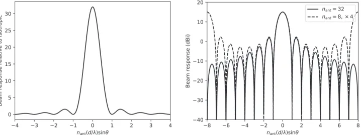
Note that, unlike a continuous square aperture, the beam in Equation (36) has aliases—additional directions of high
response—for sinqs-sinq equal to multiples of l d. We show this beam shape in Figure1.
Table 2
Summary of Classes of Beams Discussed Name Symbol Section References Description
Factorizable beam bf 3.1 Class of beams that can be formed pre-correlation on antenna signals.
Pointed beam bp( ˆ )np 3.1 Maximum response to direction ˆnp. Factorizable for identical antennas.
Optimal pointed beam bopt( ˆ )ns 3.1 Maximum S/N to source at sky location ˆns, same as pointed beams for the simple noise model.
FFT beams bA 3.2 Efficiently formed set of beams for redundant arrays. Factorizable and equivalent to pointed beams at
fixed pointing angles qA.
Naive windowed beam bnw 4.1 Antenna space tapered aperture for suppressing sidelobes. Factorizable.
While in the simple noise model, the error in the visibilities is uncorrelated, the error in pointed beams is not, and
å
q q n n p l q q p l q q ¢ = D D = D D - ¢ - ¢ p l q q - - - ¢ ( ( ) ( )) [ ( )( )] [ ( )( )] ( ) ( ) ( )( )( ) b b T t n e T t n n d d Cov 11 sin sin sin
sin sin sin
simple noise . 38 p p p p r ab i a b d r p p p p 2 ant 2 2 sin sin 2 ant2 2 ant 2 p p
This has a similar functional form to the beam shape (Equation (36)). It is zero if (sinqp-sinq¢p) is a multiple of l (nantd)and nontrivial otherwise.
Equation (35) hints that many beams could be efficiently
formed using a spatial FFT of the pre-correlation antenna signals, h [ ]a t. One can form M beams by zero padding the nant
antenna to length M and taking an FFT in the spatial direction (over index a). IfM<nantbeams are desired, then, rather than
zero padding, the array should be populated by cyclically coadding the signals from the antennas. That is, the Athelement
of the array to be Fourier transformed should be the sum of all of the ha witha(mod M)=A. We then have
å å
q = h - p ( ) [ ] ( ) b n t n e 1 1 , 39 p A t a a i Aa M samp ant 2 2noting that the inner sum over a is an FFT. The equivalent voltage beamforming weights are
q = - p ( ) / ( ) w n e 1 , 40 p a A i Aa M ant 2
and the discrete steering angles of the formed beams are
q = Al ( )
Md
sin A . 41
This equation is valid for any A satisfying the constraint
q
∣sin A∣ 1, with those outside the 0 to M-1 range describing aliases of the A(mod M)beams. We will thus refer tobp( )qA (hereafter simply bA) as the Fourier transform beams
or FFT beams. Note in the above equation that the locations of
the beams are wavelength-dependent, so, without modification, the FFT beams are not appropriate fan beams for searches for broadband point sources such as FRBs. If M=nant, then the
beams have independent errors for the simple noise model (Equation (38)), but this is not the case in general.
3.3. Redundancy-stacked Visibilities Equation(33) can be rewritten as
å
q = ~ d pd l q d =- -( ) ( ) ( ) ( ) b n e V 1 , 42 p p n n i d ant 1 1 2 sin p ant ant whereå
º ~ d a d d a d a = -+ ( ) ( ) ( ) V V . 43 n n max 0, min ant, antHereδ indexes the difference between two feed indices -a b, and the a index runs over the redundant pairs(we use a over a to make it clear that the index limits are different and dependent on δ). The quantityV is the sum of thed nant- ∣ ∣d visibilities
whose baselines are redundant. Note that because the sky contribution to the visibilities is the same for redundant baselines (Vab depends only on a− b),V contains all of thed
information in a redundant array in the case of the simple noise model where the visibilities are uncorrelated. This is not the case for nontrivial noise or nonnegligible contributions to the visibility uncertainty from the sky, where the visibilities are correlated (Equation (16)), and that correlation is
visibility-dependent even among redundant pairs. That is, the correlation between Va=2,b=1 and Va=3,b=2 will not be the same as that
betweenVa=2,b=1 and Va=4,b=3, and an optimal sum of these
three visibilities must take into account these correlations. To get an idea of how severe the information loss could be, we have considered toy models where visibilities are dominated by a single sky structure resolved by roughly half the baselines. We find that the increase in uncertainty on the stacked visibilities can be of order unity compared to an optimally weighted stack. However, the information loss remains to be quantified for a realistic sky and instrument.
Figure 1.Response function of the beamformed visibilities for a regular linear array with 32 elements on linear(left) and logarithmic (right) scales, neglecting the primary antenna response(assuming ( ˆ)Ain is isotropic). The horizontal axis is scaled to be in units of the natural beamwidth l (n d)
ant . To illustrate the effects of
Nonetheless, these correlations are small in most systems where the autocorrelations ( =a b) are much larger in amplitude than the cross-correlations ( ¹a b). We will thus assume thatV contains essentially all of the information fromd the array hereafter. As such, most beams of interest can be formed directly in this space. We will denote the weights in such cases as17w , such thatd b=w V .dd
These are trivially related to beamforming weights in unstacked visibility space:
=
d = +a d =a ( )
w wa ,b . 44
For the Fourier transform–formed beams, Equation (42)
becomes
å
å
= = ~ p d p d d - -- ( ) ( ) b n e V n e V 1 1 . 45 A ab i A a b M ab i A M ant 2 ant 2Equation(45) indicates that forM 2nant -1,bp( )qA andVd are related by a discrete Fourier transform(withV zero paddedd to length M). Since Fourier transforms are invertable, bA
contains the same information asV . That the minimum numberd of FFT-formed beams for which this is true isM =2nant-1 agrees with the number of degrees of freedom inV . Becaused
* =
d -d
V V , there are nant independent but complex numbers.
SinceVd=0 is real, there are2nant-1degrees of freedom. The
number of independent beams can also be understood in terms of the convolution theorem, where squaring the spatially transformed uncorrelated input signals is equivalent to a spatial autoconvolution of those signals. Padding to 2nant-1 is required to deal with the nonperiodicity of the antenna array. This also makes it clear that padding to any number larger than
-n
2 ant 1also preserves information. This is convenient, since =
M 2nant is likely more factorizable and can thus be
implemented more efficiently with an FFT.
As such, FFT beamforming provides a method to correlate the antenna signals, since the bAcan be formed using an FFT to
implement Equation (39), which scales as nantlognant rather
than nant 2
. This method contains the same information as the redundancy-stacked visibilitiesV . Both the FFT beamformingd and the redundancy stacking are information preserving in the case where the visibility autocorrelations are the dominant contributions to the visibility uncertainty, as discussed above.
Since the FFT beams have the same information content as theV , it is clear that any beam shape that can be produced ind visibility space can also be achieved by taking linear combinations of the FFT beams. This has a small computa-tional cost compared to the initial FFT beamforming due to the typically high degree of D Dt n down sampling in intensity space(here we refer to the sums over t in Equations (11), (25),
and (39)). Being able to form a beam with any shape is not
equivalent to being able to form any beam. For instance, a beam with wa=2,b=1¹wa=3,b=2 cannot be formed, since
= =
Va 2,b 1 and Va=3,b=2 each contribute to Vd=1 with equal
weight. However, such beams are clearly nonoptimal, since
= =
Va 2,b 1 and Va=3,b=2 contain the same sky information and
independent noise realizations.
Assuming hereafter that M 2nant -1, bA provides an
alternate basis for forming any beam where wab depends only on d =a-b. We will denote the coefficients in this space as wA, such that such a beam can be written as
å
= = -( ) b w b . 46 A M A A 0 1The inverse of Equation(45) is
å
= ~ d pd ( ) V n M A e b , 47 i A M A ant 2and, by substituting this equation into b =w V , it can bedd shown that
å
= d pd d ( ) w n M e w , 48 A ant i2 A M and likewise,å
= d - pd ( ) w n e w 1 . 49 A i A M A ant 2As an example of forming an arbitrarily shaped beam from the FFT beams, a pointed beam to an arbitrary steering angle qp can be formed. That is, pointed beam locations can be “regridded” to angles other than the FFT steering angles qA. Combining Equations(42) and (47), we have
q p p l q = -º -( ) [( ) ] ( ) ( ) ( ) w M n y y y d A M 1 sin 2 1 sin sin . 50 p A p p A p A p A p ant
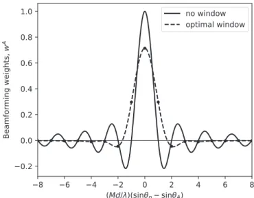
These weightswpA( )qp are beam regridding coefficients, whose functional form is also approximated by a sinc function (Equation (37)). These coefficients are shown in Figure2.
Figure 2.Weights, wA, for forming a beam pointed to an arbitrary location from FFT beams(Equation (50)). The horizontal axis has been scaled to be in
units of the separation of the steering angles for the FTT beams l (Md . The) windowed version(Equation (58), to be described in Section4.1) uses the same
half-sine-wave window as in Figure3. Note that the“naive” windowed beam cannot be formed in this space. The total number of formed beams has been set toM=2nant-1, withnant=32.
17
The symbols for beamforming weights in voltage space(wa),
redundancy-stacked visibility space(wd), and the later defined FFT beam space (wA) are
distinguishable only by the type of character used as an index. This notation is convenient, but care must be taken to not confuse the weights in different spaces.
Among other applications, this solves the location-chroma-ticity problem for fan beam implementations that use FFT beamforming, since the FFT beams can be regridded to arbitrary and achromatic steering angles on a frequency-by-frequency basis.
As afinal note, in visibility space, we have Equation (16),
which permits the covariance of the visibilities to be estimated from the visibilities themselves for arbitrary noise and sky. This is also true of the FFT-formed beams, where Equation(23) can
be used with Cabwritten in terms of á ñbA using Equation(47). This, however, does not yield a compact expression and is best calculated numerically.
3.4. Nonredundancy
Prior to delving into applications of our formalism, it is important to evaluate the validity of the assumptions made in this section. Of particular concern is the assumption of redundancy: that all antennas are equally spaced and have the same response to the sky. This may be broken due to antenna-to-antenna variations in the response functions Aa
i
, calibration errors in the analog and digital stages of the signal chains, or departures from the regularity of the antenna locations. We will analyze the effects of these variations by considering the sensitivity of a formed beam to a point source, which is the most relevant measure for time-domain radio astronomy. For illustrative purposes, we willfirst consider variations that affect the signal part of the visibilities but not the noise, such as variations in the antenna responses or departures of the antenna locations from regular spacings. Calibration errors in the analog chains multiply both signal and noise, which we will consider later.
We model the effects of these feed-to-feed variations by mapping the signal contribution to the visibilities,
˜ º g+y g-y ( )
Sabs Sab e e S , 51
s i i
abs
a a b b
where gaand yaare real numbers representing variations in the point-source response in amplitude and phase, respectively. These variations are assumed to be pertubatively small, and we use the above exponential parameterization for algebraic convenience.
We now calculate how a source’s expected contribution to a pointed beam(á ñ ºbps w Spab abs) is affected by these perturbations to the visibilities(the perturbed contribution will be denoted by á ñb˜ps
). Setting Vabto ˜Sab s
in Equation(33), expanding to second
order in the response variations, and substituting Equation(14),
we find g g g y á ñ » á ñb˜p b [1 +2¯ +2¯ + D( ) - D( ) ]. (52) s p s 2 2 2
Here g¯ º åaga nant (the mean of ga over antennas),
g g g
D º å
-( ) a( a ¯ ) n
2 2
ant (the variance), and likewise for ψ.
In the above equation, the terms with g¯ and g¯2 represent
departures of the mean response from the nominal value but do not represent antenna-to-antenna variations and thus have no bearing on the present discussion of departures from redun-dancy. The true departures affect the overall sensitivity to the source at second order; thus, the sensitivity is rather robust to these variations. For example, 10% rms variations in the amplitude response, or 0.1 rad rms variations in the phase response, affect the point-source sensitivity by 1%, a tolerable change in many applications and for a readily achievable uniformity in antenna response. Specifically, the CHIME
Pathfinder has achieved roughly 10% antenna response uniformity(Berger et al.2016). Surprisingly, variations in the
amplitude response actually increase the sensitivity to point sources, albeit by a small amount.
Likewise, calibration errors can be treated in a similar way, and, while the effect on the signal will be identical to the above calculation, the noise will also be affected. Thus, we will substitute
˜ º g+y g-y ( )
Nab Nab ea i aeb i bN .ab 53
As before, we define á ñ ºbpn w Npab ab and the perturbed version á ñb˜pn. Again we start with Equation(33), this time setting Vabto
˜
Nab and employing the simple noise model in Equation (15). Wefind
g g g
á ñ » á ñb˜p b [1+2¯ +2¯ +2(D ) ]. (54) n
pn 2 2
For the simple noise model where ábpnñá ñbps, and as a consequence of Equation(27), the S/N is
n n g y g y = D D á ñ á ñ » D D á ñ á ñ - D - D » - D - D ~ ˜ ˜ [ ( ) ( ) ] [ ( ) ( ) ] ( ) t b b t b b S N 1 1 1 S N 1 . 55 p s p n p s pn 2 2 2 2
As such, for calibration errors, the loss of point-source sensitivity is also second order in the antenna-to-antenna calibration variations.
While point-source sensitivity is not the only relevant metric, we expect other effects, such as beam shape perturbations, to be of the same order. As such, the utility of the above formalism and the applications presented below is quite robust.
4. Applications
In this section, we apply the formalism developed above to derive several observationally useful algorithms and analyze the information content of the FFT-formed beams in several contexts.
4.1. Controlling Beam Shape with Windowing In some applications, it is desirable to control the shape of formed beams to suppress the large sidelobes apparent in Figure 1. The naive way to do this is to form a factorizable beam(bnw) that windows the spatial Fourier transform such that
q ~ ( ) wa h wa p a p nw , where h
a is a window function. This
effectively tapers the illumination of the aperture (sacrificing aperture efficiency), in direct analog to how the illumination of the dish by the feed affects beam shape in telescopes that use optical focusing (Thompson et al. 2017). The resulting beam
shape is * * * * * *
å
å
å
å
q q q q q = ´ = ´ º = p l q q p l q q - - -- -⎛ ⎝ ⎜ ⎞ ⎠ ⎟ ( ) ( ) ( ) ( ) ( ) ( ) ( )( )( ) ( )( ) B A A n h h e A A n h e n h h h h n h h 1 1 1 1 . 56 jk j k ab a b i a b d j k a a i a d ab a a b b a a a nw ant 2 sin sin ant 2 sin sin 2 2 ant 2 ant 2 p pComparing to the windowed pointed beams, we see that the windowed beam shape simply replaces the sinc-squared-like factor in Equation(36) with the square of the Fourier transform
of the window (factor in ∣ ∣2).
Windowing the array in this way is, however, a suboptimal way to achieve a given beam shape, since it assigns different weights to redundant visibilities, which are independent measurements of identical sky information. Such beams cannot be formed fromV or bd A.
To form a beam with the same shape as that above but maintaining the maximum amount of sky signal (the “optimally” windowed beam, bow), we must find weights that
depend only on baseline length (i.e., d = -a b), whose sum over redundant baselines is proportional to the same sum for the above weights. That is,
* *
å
å
å
d q q d = - = = -a d d a a d a d d d a a d a + + ( ∣ ∣) ( ) ( ) ( ∣ ∣) ( ) w n w h h w w w n h h 1 , 57 p p p p ow ant ow ow antwhere the normalization does not have a simple form but is straightforward to calculate numerically for a given window
and number of elements. Notice that the factor involving a sum overα is the autoconvolution of the window function.
As an illustrative example, we use a simple half-sine wave window function given by ha =sin[p
(
a + 1)
n ]2 ant. This
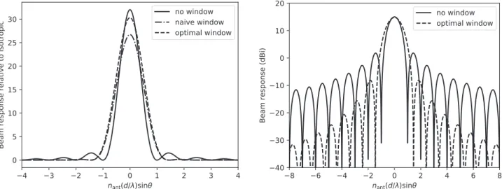
particular window function is relatively broad compared to the commonly used Hann and Blackman functions, preserving more area and thus more sky information. This is at the expense of a less gradual taper and thus inferior sidelobe suppression. The resulting sky response for both the naive window and the optimal window are shown in Figure 3. For the sine window used here, the naive windowing has 83% of the peak sky response of the unwindowed pointed beam, while the optimal windowed beam achieves 95%. The optimal window effec-tively pays a smaller aperture efficiency price for sidelobe suppression. Also, while the unwindowed and naive windowed beam shapes have the same sky area integrated response, the optimal windowed beam has 14% more, making it more sensitive to resolved extended sources and point-source searches where the flux distribution is shallower than
~( n )
-N Smin 3. This is analogous to the principle employed in
Amiri et al. (2017) to increase FRB discovery rates with the
CHIME Pathfinder using an “incoherent formed beam.” We can use Equation(48) to form the same beam from the
FFT beams bAinstead of theV . This givesd
* *
å
å
å
q d d = -= -d pd d a a d a da pd l q a d a + -+ ( ) ( ∣ ∣) ( ∣ ∣) ( ) [ ( ) ] ) w n M e w n h h n M e n h h . 58 A i A M p p i A d M ow ant 2 ant ant 2 sin ant pThe expression (nant-∣ ∣)d is proportional to the Fourier transform over A of the function in Equation(50). As such, by
the convolution theorem, dividing by this expression and the subsequent Fourier transform–like operation from δ to A amounts to a deconvolution operation on the window’s autoconvolution. These coefficients wA are shown for our example window in Figure2. We see that the windowed beam with arbitrary steering angle can be formed with a much more compact set of weights compared to an unwindowed pointed
Figure 3.Response function of formed beams for a regular linear array with 32 elements on linear(left) and logarithmic (right) scales for different windowing schemes. As in Figure1, we neglect the primary antenna response(assuming ( ˆ)Ain is isotropic). The horizontal axis is scaled to be in units of the natural beamwidth l (nantd). The beam with no windowing maximizes the sky response in the steering direction(Equation (36)) and is the identical curve as in Figure1. Naive windowing multiplies the array by a simple half-sine window function prior to voltage-space FFT beamforming to taper the aperture and control sidelobes (Equation (56)). Optimal windowing takes the combination of visibilities (Equation (32)) that achieves the same angular response as naive windowing but maximally
beam. In the case shown, a kernel of five weights obtains an excellent approximation to the full set of weights. As such, in applications where FFT beams are formed in the initial correlation and then regridded in a post-processing step, the regridding will be computationally more convenient for these optimal windowed beams.
A key point is that if we form a full set of M optimal windowed beams, this is an invertable operation on the redundancy-stacked visibilities. That means that the set of optimal windowed beams also contains the same sky informa-tion as the redundancy-stacked visibilities.
As previously mentioned, the uncertainties in any set of formed beams are, in general, correlated. This somewhat obscures how the sky information is distributed among the beams. For instance, if attempting to measure theflux of a point source not located at one of the FFT steering angles, it is not clear exactly how that information is distributed among the beams. Figure2 indicates that, to form the beam that contains all of the information, one needs to take a slowly converging sum over all of the FFT-formed beams, even while it is clear from Figure 3 that only a small number of those beams have significant sensitivity to the location of the source. To get a sense of how the information is distributed among the beams, we calculate the cumulative sensitivity of a set of beams to an unpolarized point source at angle qs, which, in the simple noise model, is given by
å
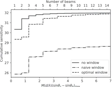
n d q d q = D D -( ) ( ) ( ) t T B C B S N . 59 r XY jk X jk s XY lm Y lm s 2 2 1In Figure4, we plot this as a function of the number of beams included in the sum. We see that while the optimal windowed beams have more compact regridding kernels in Figure 2, the unwindowed pointed beams have more compact net informa-tion. That the unwindowed pointed beams have more net information than the windowed beams at a fixed number is
unsurprising, since the unwindowed beams have a narrower main lobe and are optimal with no shape constraints, in contrast to the“optimal windowed beams.”
4.2. Noise Correlated between Antennas
We have so far mostly assumed the simple noise model given in Equation(15). Here we will briefly consider simple,
physically motivated departures from this model, what effect they have on sensitivity, and how the optimal beamforming weights are affected.
One simple case is where the noise continues to dominate the sky and remains uncorrelated but the receiver temperature, Tr,
is feed-dependent. This is expected to result from variations in the properties of the amplifiers among the analog chains for each feed. A quick look at Equation(32) shows that the optimal
pointed beam can be formed by weighting the voltages by the inverse receiver temperature, which can conveniently be done pre-correlation/pre–beamforming. If this weight is applied before FFT beamforming, then the sky response of bA is
modified, but they remain the maximum-sensitivity beams to the same steering angles qA, and they still contain all of the sky information. The Fourier transform of bAbecomes a modified
version ofV , where redundant visibilities are coadded withd optimal S/N-square weights instead of uniform weighting.
Another well-motivated noise model includes “cross talk”: noise coupling between nearby feeds. Such a model can be written
x
= d= - ( )
Nab Tr a b, 60
where xd is the noise correlation kernel. We will take x = 10 , *
x-d=xd and assume that it is compact: the correlations are negligible except for d ∣ ∣ nant. Under the assumption of
redundancy, for each noise contribution that couples from antenna a to antenna b, there should be an equal contribution that couples from b to a with the opposite phase. As such, the imaginary part of xa-bshould be zero, although we present the more general case. If we approximate the array as being periodic, Nabcan be inverted analytically, allowing us to take
its inverse in the spatial Fourier domain. Define
å
x q º x d pd l q d = -( ) e ( ) . (61) n i d 0 1 2 sin antThen, it can be shown that
å
x q l » = p -= - -( ( )) ( ) ( ) N n T e A n d 1 sin . 62 ab r A n i a b A n 1 ant 0 1 2 ant ant antThe approximation improves as xd becomes more compact compared to nant, since edge effects from the assumed
periodicity become less significant. From this, it can be shown that the optimal weights given in Equation (32) are just the
normal pointed beam weights,wpab( )qp, with no modifications. However, the variance of these beams gets modified by the correlations * q n x q x q = D D [b ( )] T ( ) ( ) ( ) t Var p p r p p . 63 2
As such, cross talk induces sky directions of lower sensitivity. Because xd is typically real-valued, the loss of sensitivity will be strongest in the zenith direction.
Figure 4.Cumulative sensitivity to an unpolarized point source as a function of the number of regularly spaced beams included. The point source is located1
4
beam spacing from zenith, and the cumulative sensitivity is plotted as a function of the maximum distance from the source to the steering angle, scaled to units of the beam spacing l (Md . We assume the simple noise model in) Equation (15). Sensitivity is relative to an isotropic antenna with
=
-M 2nant 1andnant=32. We consider arrays of beams of the same three
Note that sky contributions to the total covariance have a similar effect as cross talk, since for a redundant array, Sabalso
only depends on a−b. In this analog, Trx q( ) I( )q . However, there is no reason to think Sab will be especially
compact in a−b, and as such, it is unclear if our analytic matrix inversion is at all valid.
4.3. Localization
One common use of multibeam systems is to determine the sky location of a source detected in one or more beams. This is especially true in searches for fast radio bursts, where follow-up of the transients is usually impossible. Here we will derive the optimal maximum-likelihood estimator for the sky location for the case where the formed beams are the M FFT beams of a redundant array bA. One place where this is particularly useful
is in triggered baseband recoding systems, where we have the freedom to correlate the data in any way we see fit, but FFT beamforming can be done efficiently. We will briefly discuss general sets of formed beams at the end of the section.
Define bXsas the contribution to beam bXfrom a point source,
which we assume can be cleanly separated from backgrounds (e.g., in the time domain for transients or radio spectrum for lines). Combining Equations (8) and (21), we have
* d n n n d n á ñ = = n p n ( ˆ ) ( ˆ ) ( ˆ ) ( ) · ˆ n n n b B c k S w e A A c k S 2 , , 2 . 64 u n Xs jk X jk s B s Xab i a j s b k s jk B s 2 2 2 2 2 ab s
Our goal is to estimate ˆns, noting that there is a second unknown parameter, the fluxSns, with which the location may be degenerate.
The log likelihood is
å
c = -= - - á n ñ - - á n ñ [ ( ˆ ) ] [ ( ˆ ) ] ( ) n n b b S b b S ln 1 2 1 2 , , , 65 XY Y s Y s s s YX X s X s s s 2 1where XY should be estimated using a sky and noise model. Alternatively, it could be estimated directly from the data using Equation(23), should the visibilities—or in redundant arrays,
d ˜
V or bA—be available. We would like to find the value of ˆns and Sns that maximizes this likelihood(minimizes c2).
From here, we restrict ourselves to the case where the beams are the FFT beams in a redundant array and to the simplified noise model. We define TsºA Aj k*d n Sn
jk c k s 2B 2
2 and use this
rather than the flux to parameterize the source strength. Note that while the primary beam sky response, Ai, depends on the unknown source location, this dependence is assumed to be weak compared to the interferometric phases. The validity of this assumption will depend on the instrument’s antenna response and array configuration. For CHIME, this is likely an excellent approximation in the north–south directions but may be invalid east–west. As such, we will ignore the small amount of information contained in this dependence. For our deriva-tion, we will initially work withV rather than b˜d A, since they are
uncorrelated in the simple noise model. Thus, Equation (18)
(scaled by the stacking factor nant- ∣ ∣d) can be used for the
covariance. We then have
*
å
å
c n d n d d =D D - á ñ - á ñ -=D D - -d d d d d d d pd l q [ ( ˆ ) ][ ( ˆ ) ] ∣ ∣ ∣ ( ∣ ∣) ∣ ∣ ∣ ( ) ( ) n n t T V V V V n t T V n T e n . 66 r s s s s s s r s s i d 2 2 ant 2 ant 2 sin 2 ant sWe will use Newton’s method to find the minimum. This requires thefirst and second derivatives of c2 with respect to
q
sin s. These are
å
c q n l pd ¶ ¶ = D D d d p l d q -( ) ( ) ( ) tT T d i V e sin 2 2 , 67 s s r s i d 2 2 2 sin så
c q n l pd ¶ ¶ = D D d d p l d q -( ) ( ) ( ) ( ) tT T d V e sin 2 2 . 68 s s r s i d 2 2 2 2 2 2 2 2 sin sThe Newton’s method estimator forsinqs, which we denote assinqs, is then
å
å
q q c q c q q l d p pd = - ¶ ¶ ¶ ¶ = -´ d d p l d q d d p l d q - ⎡ ⎣⎢ ⎤ ⎦⎥ ⎡ ⎣ ⎢ ⎤ ⎦ ⎥ ( ) ( ) ( ) ( ) ( ) d i V e V e sin sin sin sin sin 2 2 , 69 s s s s s s i d s i d 2 2 2 2 1 2 sin 2 2 sin 1 s swheresinqsis to be evaluated at the current best guess for the location, and the estimator should be applied iteratively until it converges. Note that Tscancels, so there is no degeneracy with
the sourceflux (except from the primary beam, which we have explicitly ignored). This should be generically true anytime the complete array information, in the form of either Vab,V , or b˜d A,
is available. Inspecting the above formula gives some insight into how the estimator operates. The first factor of the update term tells us to form the beam whose sky response is the derivative of the pointed beam with respect to steering angle qs. The factor in square brackets tells us to form the beam whose sky response is the curvature(second derivative) of the pointed beam with steering angle qs.
Armed with this form, we can proceed to make improve-ments to the simple Newton’s method estimator. First, Newton’s method assumes that the curvature is constant, or at least slowly varying between the initial guess and the true maximum. Inspecting the beam shape for the pointed beam in Figure 1, we see that there is actually an inflection point roughly a quarter beamwidth from the maximum. Thus, we are almost certainly better off replacing the curvature at the initial guess with the curvature at the maximum, properly scaled for the best estimate of theflux. That is,