Present and future impact of aircraft, road traffic and shipping emissions on global tropospheric ozone

HAL Id: hal-03049270

https://hal.archives-ouvertes.fr/hal-03049270

Submitted on 10 Dec 2020

HAL is a multi-disciplinary open access

archive for the deposit and dissemination of

sci-entific research documents, whether they are

pub-lished or not. The documents may come from

teaching and research institutions in France or

abroad, or from public or private research centers.

L’archive ouverte pluridisciplinaire HAL, est

destinée au dépôt et à la diffusion de documents

scientifiques de niveau recherche, publiés ou non,

émanant des établissements d’enseignement et de

recherche français ou étrangers, des laboratoires

publics ou privés.

shipping emissions on global tropospheric ozone

B. Koffi, S. Szopa, A. Cozic, D. Hauglustaine, P. van Velthoven

To cite this version:

B. Koffi, S. Szopa, A. Cozic, D. Hauglustaine, P. van Velthoven. Present and future impact of aircraft,

road traffic and shipping emissions on global tropospheric ozone. Atmospheric Chemistry and Physics,

European Geosciences Union, 2010, 10 (23), pp.11681-11705. �10.5194/ACP-10-11681-2010�.

�hal-03049270�

www.atmos-chem-phys.net/10/11681/2010/ doi:10.5194/acp-10-11681-2010

© Author(s) 2010. CC Attribution 3.0 License.

Chemistry

and Physics

Present and future impact of aircraft, road traffic and shipping

emissions on global tropospheric ozone

B. Koffi1, S. Szopa1, A. Cozic1, D. Hauglustaine1, and P. van Velthoven2

1_{Laboratoire des Sciences du Climat et de l’Environnement, UMR 8212, IPSL, CEA-CNRS-UVSQ,} Gif-sur-Yvette, France

2_{Royal Netherlands Meteorological Institute, KNMI, De Bilt, The Netherlands} Received: 30 May 2010 – Published in Atmos. Chem. Phys. Discuss.: 28 June 2010

Revised: 17 November 2010 – Accepted: 21 November 2010 – Published: 9 December 2010

Abstract. In this study, the LMDz-INCA climate-chemistry

model and up-to-date global emission inventories are used to investigate the “present” (2000) and future (2050) impacts of transport emissions (road traffic, shipping and aircraft) on global tropospheric ozone. For the first time, both im-pacts of emissions and climate changes on transport-induced ozone are investigated. The 2000 transport emissions are shown to mainly affect ozone in the Northern Hemisphere, with a maximum increase of the tropospheric column of up to 5 DU, from the South-eastern US to Central Europe. The impact is dominated by road traffic in the middle and upper troposphere, North of 40◦S, and by shipping in the northern lower troposphere, over oceanic regions. A strong reduction of road emissions and a moderate (B1 scenario) to high (A1B scenario) increase of the ship and aircraft emissions are pro-jected by the year 2050. As a consequence, LMDz-INCA simulations predict a drastic decrease in the impact of road emissions, whereas aviation would become the major trans-port perturbation on tropospheric ozone, even in the case of a very optimistic aircraft mitigation scenario. The A1B emis-sion scenario leads to an increase of the impact of transport on zonal mean ozone concentrations in 2050 by up to +30% and +50%, in the Northern and Southern Hemispheres, re-spectively. Despite a similar total amount of global NOx emissions by the various transport sectors compared to 2000, the overall impact on the tropospheric ozone column is in-creased everywhere in 2050, due to a sectoral shift in the emissions of the respective transport modes. On the oppo-site, the B1 mitigation scenario leads to a significant reduc-tion (by roughly 50%) of the ozone perturbareduc-tion throughout the troposphere compared to 2000.

Correspondence to: B. Koffi

(brigitte.koffi@lsce.ipsl.fr)

Considering climate change, and according to scenario A1B, a decrease of the O3tropospheric burden is simulated by 2050 due to climate change (−1.2%), whereas an in-crease of ozone of up to 2% is calculated in the upper tro-posphere in the inter-tropical zone, due to enhanced light-ning activity. A global impact of similar magnitude is sim-ulated for the transport-induced ozone burden perturbation (−1.6%). As a result, the future increase in global ozone due to changes in anthropogenic emissions is lowered by 12% and by 4%, for the background and the transport-induced ozone, respectively. However, positive and negative climate effects are obtained on ozone, depending on the season, re-gion and altitude, with an increase of the transport-induced ozone perturbation (+0.4 DU) in the already most affected area of Northern Hemisphere.

1 Introduction

Emissions from the transport sectors contribute globally for about 30% to 40% to global anthropogenic emissions of carbon monoxide and nitrogen oxides, respectively, and to about 25% of anthropogenic Non Methane Hydrocarbon Compounds, NMHCs (e.g., Olivier at al., 2005). In the atmosphere, CH4, CO and NMHCs in presence of NOx act as ozone precursors by forming radicals which finally contribute to the ozone formation (Crutzen et al., 1999) and therefore, indirectly impact on climate. Fuglestvedt et al. (2008) found that transport has contributed to 31% of the total man-made O3forcing, since preindustrial times. Unger et al. (2008) calculated that transport emissions in Europe and North America have a particularly large forcing and are therefore attractive targets to counter global warming. The chemical production of ozone is a highly non-linear function of emitted NOxand NMHC precursors, and is very sensitive

to local meteorology and atmospheric background composi-tion. Besides their effect on the ozone concentration and its related radiative forcing, the emissions from transport also affect the OH concentration, i.e. the oxidizing capacity of the atmosphere (e.g., Niemeier et al., 2006). The emissions by the transport sector are expected to show drastic quanti-tative and geographic changes in the next decades, which in turn will affect air quality and climate (Kahn Ribeiro et al., 2007). Moreover, significant changes in climate conditions are expected to occur in the future (Meehl et al., 2007), af-fecting the atmospheric oxidation processes (Hedegaard et al., 2008), and thereby, possibly, the atmospheric perturba-tions induced by transport emissions.

In the last decade, several atmospheric model studies were performed to assess the global impact of present-day trans-port emissions on the chemical composition of the atmo-sphere, but focusing on a given transport mode.

The impact of NOx and CO current road emissions was first investigated by Granier and Brasseur (2003), who esti-mated their relative contribution between 12% and 15% and of about 9% of the ozone background near the surface, in industrial and remote regions, respectively. More recently, Matthes et al. (2007) concluded that the maximum relative impact of road traffic emissions (NOx, CO, NMHC) occurs at Northern mid-latitudes in July, contributing by up to 16% and 12% of the surface and zonal mean ozone concentra-tions, respectively. They also demonstrated the important role of NMHC that contribute to an indirect long-range trans-port of NOx from road traffic via the formation of PAN, and consequently, lead to a greater influence on ozone in re-mote areas (i.e., by +30%). Similar results were also ob-tained by Niemeier et al. (2006) who concluded that the road traffic emissions increase the zonally averaged tropospheric ozone concentration by more than 10% in the boundary layer, and by about 6% at 500 hPa and 2.5% at 300 hPa, in July. Niemeier et al. (2006) and Matthes et al. (2007) reported changes in the July ozone surface concentration by 20% and by up to little more than 16% in source regions, respectively. Many model studies investigated the present impact of international shipping on atmospheric chemistry, and more specifically on ozone (Lawrence and Crutzen, 1999; Cor-bett and Kohler, 2003; Endresen et al., 2003, 2007; Eyring et al., 2005a, 2007; Huszar et al., 2010). They underlined that ozone perturbations due to shipping is highly nonlin-ear, being most efficient in regions of low background pol-lution. These studies suggest an overall higher ozone pro-duction efficiency of NOxship emissions, compared to road traffic emissions. However, they also mentioned important uncertainties associated to the total amount of emissions, the neglect of ship plume dispersion, and their spatial distribu-tion. More recently, Dalsoren et al. (2009) calculated the im-pact from the international fleet of ships using updated emis-sions datasets from the EU QUANTIFY project (Quantifying the Climate Impact of Global and European Transport Sys-tems; http://www.pa.op.dlr.de/quantify/). They found that

ship emissions contribute for a large part to surface ozone over the oceans (up to 40%), but also over some continental areas such as over Western America (15–25%) and Western Europe (5–15%). A contribution up to 5–6% to the tropo-spheric ozone column was simulated over the North Atlantic. Huszar et al. (2010) found that the contribution of ship in-duced surface NOxto the total background reaches 90% over remote ocean, and makes 10–30% near coastal regions. They calculated that due to ship emissions, surface ozone increases by up to 4–6 ppbv, making 10% contribution to the surface ozone budget.

The global impact of NOx emissions from subsonic air-craft on ozone has been extensively investigated (Hauglus-taine et al., 1994; Brasseur et al., 1996, 1998a; Wauben et al., 1997; Stevenson et al., 1997; Schumann, 1997; Schumann et al., 2000; Dameris et al., 1998; Kentarchos and Roelofs, 2002; Grewe et al., 2002; Gauss et al., 2006; Cariolle et al., 2009). While representing less than 2% of the global current NOxemissions, the aircraft emissions are shown to lead to a significant ozone perturbation in the Upper Troposphere and Lower Stratosphere (UTLS), i.e., where NOx have a much higher ozone production potential than at Earth’s surface, and where increases in ozone are known to cause an impor-tant radiative forcing (e.g., Sausen et al., 2005; Lee et al., 2009). First studies calculated for instance an increase by 2 up to 8% of the ozone background (Brasseur et al., 1998a). However, large differences, in both magnitude and seasonal-ity, were highlighted between the different studies, resulting notably from the lack of NMHC chemistry, the coarse verti-cal resolution at the tropopause, quantitative uncertainties on NOx emissions by lightning and mass transport by convec-tion (Grewe et al., 2002). More recently, Gauss et al. (2006) found a maximum increase in the monthly averaged zonal mean ozone in June (+7.6 ppbv) and a minimum in Septem-ber (∼3 ppbv), and increase of 6 ppbv for July. Last results from the NMHC version of the LMDz-INCA model, using AERO2K 2002 emissions (Eyers et al., 2004) show lower changes and different spatial patterns, with a maximum per-turbation of 3.5 ppbv in spring, and an increase of 2.6 ppbv for July (Cariolle et al., 2009). This last study and Huszar et al. (2010) study more especially focused on the assess-ment of plume sub-grid effects. They calculated that the non-linear chemistry which takes place in the plume dispersion leads to a decrease of the aircraft and the shipping-induced ozone production, by 10 to 15% (free troposphere of North-ern Hemisphere) and by 15 to 30% (surface ozone over the Eastern Atlantic), respectively.

For the first time, the combined effects of the three modes of transport and their respective influence on the current com-position of the atmosphere have been recently investigated at the global scale, in the framework of the QUANTIFY project. A multi-model analysis based on 2000 preliminary road and aircraft (AERO2K 2002) emissions has been per-formed (Hoor et al., 2009). It provides a detailed interpreta-tion of the chemical and transport processes involved in the

ozone and OH current perturbations by the three transport modes, and the related radiative forcing, as well as an assess-ment of uncertainties due to the different models formula-tion. While differences were obtained in the magnitude of the impacts, similar results were simulated by the 6 global chem-istry models involved (including LMDz-INCA), in terms of geographical patterns and respective contributions by the dif-ferent transport modes. The mean results are also consistent with previous studies for aircraft and shipping, whereas the predicted road perturbation was found to be lower than previ-ously reported in the literature. The authors attributed the dif-ferences to a significant under-estimation of the preliminary road emissions. Their study also highlighted that uncertain-ties between the models are larger in summer than in winter, with a maximum zonal mean ozone perturbation at 250 hPa ranging from 3.5 ppbv for LMDz-INCA model to 6 ppbv for p-TOMCAT model, for July. In fact, the LMDz-INCA model is known to simulate relatively low tropospheric ozone pro-duction in summer compared to other models, due to particu-larly intense convection and associated dilution effect during this season.

While the impact of futures changes in anthropogenic emissions on background tropospheric ozone has been widely documented (e.g., for the most recent ones, Hauglus-taine et al., 2005; Gauss et al., 2006; Niemeier et al., 2006; Granier et al., 2006; Eyring et al., 2005b, 2007; Stevenson et al., 2006; Søvde et al., 2007; Wu et al., 2008), only few of them specifically dealt with transport emissions, mainly because no reliable detailed emission scenarios for the next 100 years were available. Therefore, most of them are sensitivity rather than prediction studies. Moreover, as for present emissions, they focused on a specific transport mode. Niemeier et al. (2006) assumed road emissions in all regions of the world to be, on a capita basis, the same as in Europe and in the United-States. In the latter and most dramatic case, they calculated an increase by up to 50–100% (south Asia) of the surface ozone concentration compared to the present situation. Granier et al. (2006) analyzed the potential im-pact of changes in shipping routes in the Arctic region due to sea ice reduction induced by climate change. They found that the surface ozone concentration could increase during summertime to ozone levels comparable to the values cur-rently observed in many industrialized regions of Northern Hemisphere. Eyring et al. (2007) analysed the impact of a constant annual growth rate of 2.2% of ship emissions up to 2030. They found a contribution of 2030 shipping emis-sions of up to 8 ppbv and 1.8 DU for the annual mean near-surface ozone and the ozone column, respectively. Gauss et al. (2006) investigated the effects of enhanced air traffic along polar routes, and of potential changes in cruising alti-tudes. They concluded that an enhanced use of polar routes would lead to a significant increase in the zonal mean ozone concentration at high Northern latitudes in summer, but to a negligible effect in winter. They also found that raising flight altitudes increases the ozone burden both in the troposphere

and lower stratosphere, whereas lowering the flight altitude has a contrasting effect depending on the altitude (decrease of ozone production in the UTLS and increase below). Finally, Søvde et al. (2007) used a 2050 NOx global aircraft emis-sions dataset from the EU project SCENIC. They calculated that the subsonic aircraft emissions could be responsible for an increase by up to 10–17 ppbv of O3in annual/July zonal mean in the UTLS of the Northern Hemisphere.

In addition to changes in emissions, the global tropo-spheric chemistry will be affected in the future by climate change (e.g., Hauglustaine et al., 2005; Isaksen et al., 2005; Brasseur et al., 2006; Liao et al., 2006; Murazaki and Hess, 2006; Stevenson et al., 2006; Grewe, 2007; Hedegaard et al., 2008; Wu et al., 2008). Most of the processes involved in the tropospheric chemistry depend notably on tempera-ture, humidity and cloud cover. Because of a global tem-perature change, atmospheric transport and mixing proper-ties in the atmospheric boundary layer will also be affected. The emission of NOx by lightning is also expected to in-crease with increasing convection. The atmospheric chem-ical reactions and photolysis rates will be modified because of changes in humidity and global radiation. Moreover, the liquid water content, the precipitation frequency and amount as well as the surface properties affect wet and dry deposi-tion levels. All the previous studies showed that future cli-mate change will lead to an increase in water vapor and OH at global scale. This increase in OH within the troposphere will contribute to a significant change in the typical life time of many species, since OH is participating in a large number of chemical reactions. As a result of enhanced water vapour, a decrease in future global ozone burden, but with positive and negative ozone changes according to altitude, season, model, and the reference year or the scenario are generally predicted (e.g., Wu et al., 2008, and references inside). Pre-vious studies also showed that the changes in tropospheric ozone are not only dominated by tropospheric chemistry, but also by the stratospheric ozone budget and its flux into the troposphere, which could increase by 2100 because of cli-mate change (e.g., Hauglustaine et al., 2005; Isaksen et al., 2005; Murazaki and Hess, 2006).Whereas all these previ-ous studies focused on changes in the ozone background, the present study analyses the impact of climate change sepa-rately for the background ozone and for the ozone generated by the transport emissions. The hypothesis here is that the above-mentioned climate-induced physical and chemical at-mospheric changes will also have a significant influence on the impact of the emissions from the transport sector.

Since the tropospheric impact of transport emissions is ex-pected to show important changes in the next decades, be-cause of changes in both emissions and climate, it is essential to assess such future changes, in order to implement adequate regulations and incentives. In this study, the LMDz-INCA model is used to study the impact of both present and future transport emissions, based on the QUANTIFY final updated emission datasets (Borken-Kleefeld et al., 2010). Our main

objectives are (i) to quantify the contribution of each of the three sectors (road traffic, shipping and aircraft) to the ozone background concentrations, and (ii), for the first time, to eval-uate the effects of future climate change on this transport im-pact. The following section describes the LMDz-INCA mod-eling system, focusing on its recent improvements (Sect. 2). The emissions, modeling and experiments are then presented (Sect. 3) and the simulation results are discussed (Sect. 4). Finally, conclusions are provided in Sect. 5.

2 The Chemistry-Climate Model LMDz-INCA

The global Climate Chemistry Model LMDz-INCA consists of the LMDz (Laboratoire de M´et´eorologie Dynamique) General Circulation Model (Sadourny and Laval, 1984; Le Treut et al., 1994, 1998), coupled with the chemistry and aerosol model INCA (Interaction with Chemistry and

Aerosols) in order to represent the chemistry of the

tropo-sphere (Hauglustaine et al., 2004; Folberth et al., 2006). The version of the LMDz model used here (LMDz 4.0) is described in Hourdin et al. (2006). It has 19 hybrid levels on the vertical from the ground to 3 hPa and a horizontal resolu-tion of 2.5◦in latitude and 3.75◦ in longitude (96 × 72 grid cells). The large-scale advection of tracers is performed us-ing the finite volume transport scheme of Van Leer (1977), as described in Hourdin and Armengaud (1999). The turbulent mixing in the planetary boundary layer is based on a second-order closure model. In the present study, the Emanuel scheme (Emanuel, 1991, 1993) was used for convection. The primitive equations in LMDz are solved in 3 min time-step, large-scale transport of tracers is carried out every 15 min and physical processes are calculated at a 30 min time interval.

The INCA model is coupled on-line to the LMDz gen-eral circulation model. INCA considers the surface and 3-D emissions, calculates dry deposition and wet scavenging rates, and integrates in time the concentration of atmospheric species with a time step of 30 min. INCA uses a sequential operator approach, a method generally applied in chemistry-transport-models (Muller and Brasseur, 1995; Brasseur et al., 1998b; Wang et al., 1998; Poisson et al., 2000). In addi-tion to the CH4-NOx-CO-O3photochemistry representative of the tropospheric background (Hauglustaine et al., 2004), the non-methane hydrocarbon version of INCA used in this study (version NMHC.3.0) takes into account the photo-chemical oxidation pathways of non-methane hydrocarbons and non-methane volatile organic compounds from natural and anthropogenic sources, as well as their photochemical oxidation products. Unlike Cariolle et al. (2009), the plume effects from the transport emissions are not taken into ac-count in the present study. For a more detailed description of the INCA-NMHC chemistry model, we refer to Folberth et al. (2006). A zonally and monthly averaged ozone climatol-ogy is prescribed above the tropopause (150 hPa), based on Li and Shine (1995). This climatology is deliberately kept

fixed at present-day values in all simulations in order to iso-late the effects of tropospheric chemistry and climate change to changes in the stratospheric chemistry. Regardless the pre-scribed stratospheric ozone climatology, the stratosphere to troposphere exchanges are affected by changes in the verti-cal circulation across the tropopause.

The LMDz-INCA chemical results were compared to many other global CTMs or GCMs, and to observations dur-ing the international HTAP (Hemispheric Transport of Air Pollution) and ACCENT/PhotoComp (Atmospheric Compo-sition Change: the European NeTwork of excellence) exer-cises. The related papers show a response (in term of sen-sitivity to emissions) of LMDz-INCA which is quite simi-lar to the ensemble mean of the results for ozone (Steven-son et al., 2006). Comparisons with ozone surface net-work (Ellingsen et al., 2008) show a systematic positive bias for all the models, partly due to misrepresentation of NOx gradient close to the sources. Reidmiller et al. (2009) and Fiore et al. (2009) tried to discriminate the climato-logic feature of ozone measured by the CASTNET (Clean Air Status and Trends Network; USA) and EMEP (Euro-pean Monitoring and Evaluation Programme) networks be-fore comparing with global models. LMDz-INCA showed in these studies a fairly good agreement for ozone with US stations. More recently, Jonson et al. (2010) compared 12 models involved in the HTAP experiment to ozone sonde measurements and concluded that the global models have far more difficulty in accurately reproducing ozone variability in the free troposphere. As stated by Shindell et al. (2006), all the global models show large under-estimates of North-ern Hemisphere extra-tropical CO, while typically perform-ing reasonably well elsewhere. An evaluation of the per-formance of the global chemistry transport and chemistry-climate models involved within the QUANTIFY project has also been performed (Schnadt et al., 2010), using observa-tions from the long-term programme MOZAIC (Measure-ments of OZone, water vapour, carbon monoxide and nitro-gen oxides by in-service AIrbus airCraft), as well as from the SPURT (Trace gas transport in the tropopause region), CON-TRACE II (Convective Transport of Trace Gases into the Upper Troposphere over Europe) and TROCCINOX Tropi-cal Convection, Cirrus and Nitrogen Oxides) campaigns. In accordance with the previous conclusions, the ozone con-centrations are shown to be over-estimated at northern mid-latitudes by the present version of LMDz-INCA and the other models, whereas CO is significantly underestimated by all models throughout the troposphere, at northern mid-latitudes and in the subtropics. No systematic bias is obtained for the NOxconcentrations in the upper troposphere and lower stratosphere between LMDz-INCA simulations and the dif-ferent observation campaigns.

3 Modelling set-up

3.1 Emissions

The socioeconomic scenarios developed in the framework of the Intergovernmental Panel on Climate Change (IPCC) are commonly used as the reference to assess the future global anthropogenic emissions. All the related SRES (Special Re-port on Emission Scenarios) emission estimates (Nakicen-ovic and Swart, 2000) project a global increase in emis-sions of ozone precursors by 2050, mainly because of eco-nomic growth in developing countries. Three of them (A1B, A1T and B1) show a decrease in these emissions in Eu-rope and North America. However, these global datasets, which are commonly used by the modellers’ community to assess the impact of the emissions by the different sectors on global chemistry and climate, do not provide transport sectoral details. Furthermore, assumptions about quantita-tive and geographic changes in emissions are rapidly evolv-ing with emissions regulations, technological and market progress, and potential for non-fossil fuels. Therefore, an update was required to assess how the impact from trans-port and from individual modes will be modified in future (Uherek et al., 2010). To this purpose, it is also of great im-portance to use realistic “present” and future emissions by other emission sectors, since the ozone sensitivity to traf-fic emissions substantially depends on background precursor concentrations. All the “present” and future transport emis-sions used in this study (Table 1) were especially provided by the FP6 QUANTIFY European project, as well as fu-ture non-traffic anthropogenic and the biomass burning emis-sions (www.pa.op.dlr.de/quantify/emisemis-sions). They consist in global files, with a resolution of 1◦_×1◦_{longitude by}

lati-tude, for the years 2000 and 2050 and for two SRES marker scenarios (A1B and B1). The present non-traffic emissions are based on the latest release of the EDGAR 32FT2000 emission inventory for the year 2000 (van Aardenne et al., 2005; Olivier et al., 2005). For biomass burning, monthly means for the year 2000 were used, based on the Global Fire Emissions Database GFEDv2 (van der Werf et al., 2006) with multi-year (1997–2002) averaged data, using Andreae and Merlet (2001) emission factors, updated for NOx. The effec-tive injection height of biomass burning emissions into the atmosphere was taken into account with the emission heights as prescribed by Dentener et al. (2006).

The biogenic emissions were calculated for 2000 with the dynamical global vegetation model ORCHIDEE (Krinner et al., 2005), as described in Lathi`ere et al. (2005). While these emissions might also show very important changes in future (e.g., Lathi`ere et al., 2005, 2006), high uncertainties still re-main about their future trends (Heald et al., 2009), so that no future global biogenic emission dataset can be provided for the different future IPCC scenarios. Therefore, they are fixed to the 2000 values in all our simulation experiments, such as oceanic emissions (Folberth et al., 2006).

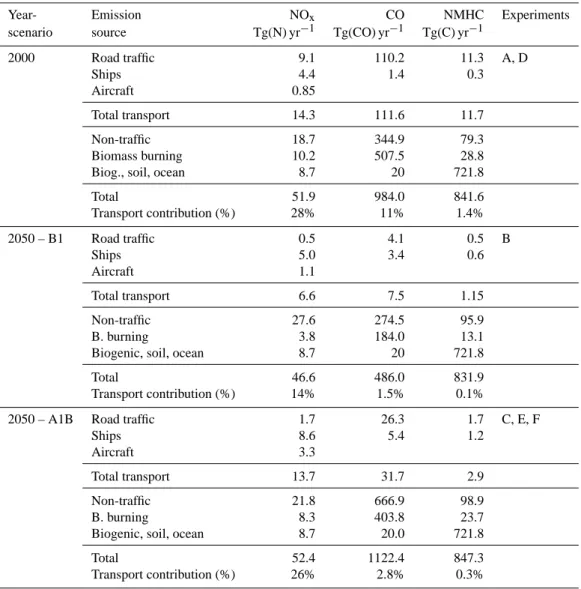
The resulting QUANTIFY 2000 final emissions from road (Table 1) are 33%, 50% and 51% higher than QUANTIFY preliminary ones (Hoor et al., 2009) for NOx, NMHC and CO, respectively. They are closer for NOx, but still lower for CO and NMHC compared to previous assessments. For comparison, the road traffic emissions adopted by Matthes et al. (2005) and Niemeier et al. (2006) for NMHC and CO are about twice the emissions used in the present study. The emissions for ship traffic are the same as Hoor et al. (2009), and were reconstructed for QUANTIFY, based on Endresen et al. (2007). Only NOx emissions are considered in the present study. They represent a total NOx annual amount (0.85 Tg N) slightly higher but with very similar spatial dis-tributions than AERO2K emission data.

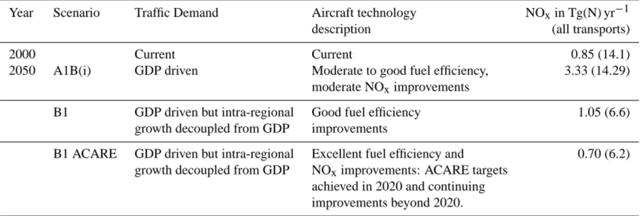
The QUANTIFY transport emissions used in this study for A1B and B1 scenarios show very important changes in the future. Spatially, transport emissions shift in absolute amounts and relative shares from OECD countries to Asia, the Middle East and South America (Uherek et al., 2010). Road traffic emission fluxes strongly decrease at global scale, whereas a moderate (B1) to high (A1B) increase of the ship and aircraft emissions are expected by 2050 (Table 1). As shipping and aviation show strongest emissions in the fu-ture, increasing amounts of pollutants are emitted in the ma-rine atmosphere and in the upper troposphere. As a result of changes in the use of the different transport modes, as well as in fuel composition, consumption and efficiency, transport-induced emissions of NOxdecrease by 20% (A1B) and 55% (B1) until 2050, whereas NMVOC and CO emissions de-cline by a factor 4 (A1B) to 10 (B1). As a result from traffic and non-traffic emissions changes, the contributions of traf-fic to NOx, NMVOC and CO total emissions decrease from 28%, 1.4% and 11% in 2000 to 26%, 0.34% and 2.8% and to 14%, 0.14% and 1.5% in 2050 for A1B and B1 scenarios, respectively. For aircraft emissions, an additional scenario (B1ACARE) based on excellent fuel efficiency is also inves-tigated (Table 3).

3.2 The perturbation approach

A small perturbation approach is used to assess the impact of transport emissions on global chemistry. For all studied scenarios, a reference simulation is first performed with all emissions. Then, the road traffic, ship and aircraft emis-sions are separately reduced by 5% in 3 additional simula-tions. The total impact of transport emissions is calculated by adding the three perturbations rather than by simulating an additional perturbation run for all transport emissions. Sensi-tivity tests performed with LMDz-INCA for 2000 emissions clearly demonstrated that the effect on ozone of small emis-sion reductions is additive: the perturbations on the ozone column and the zonal mean ozone induced by a 5% re-duction of all transport emissions differ by less than 0.3% compared to the sum of the 3 perturbations due to a 5% reduction of each transport mode. The small perturbation

Table 1. Global emissions and corresponding modelling experiments.

Year- Emission NOx CO NMHC Experiments

scenario source Tg(N) yr−1 Tg(CO) yr−1 Tg(C) yr−1

2000 Road traffic 9.1 110.2 11.3 A, D Ships 4.4 1.4 0.3 Aircraft 0.85 Total transport 14.3 111.6 11.7 Non-traffic 18.7 344.9 79.3 Biomass burning 10.2 507.5 28.8

Biog., soil, ocean 8.7 20 721.8

Total 51.9 984.0 841.6 Transport contribution (%) 28% 11% 1.4% 2050 – B1 Road traffic 0.5 4.1 0.5 B Ships 5.0 3.4 0.6 Aircraft 1.1 Total transport 6.6 7.5 1.15 Non-traffic 27.6 274.5 95.9 B. burning 3.8 184.0 13.1

Biogenic, soil, ocean 8.7 20 721.8

Total 46.6 486.0 831.9

Transport contribution (%) 14% 1.5% 0.1%

2050 – A1B Road traffic 1.7 26.3 1.7 C, E, F

Ships 8.6 5.4 1.2

Aircraft 3.3

Total transport 13.7 31.7 2.9

Non-traffic 21.8 666.9 98.9

B. burning 8.3 403.8 23.7

Biogenic, soil, ocean 8.7 20.0 721.8

Total 52.4 1122.4 847.3

Transport contribution (%) 26% 2.8% 0.3%

approach minimizes non-linearity in atmospheric chemical effects, which would occur by setting the respective emis-sions to zero. Furthermore, a small reduction in emisemis-sions is expected to be more realistic than a total decline.

Despite the non-linear character of the ozone perturba-tion, the 100% up-scaled perturbations (multiplied by a fac-tor 20) are displayed on the figures, in order to better com-pare with the results of Hoor et al. (2009) and other previ-ous studies using such up-scaling. In order to quantify the non-linear effects, and to compare with previous studies us-ing a total removal of emissions, a 100% decline of 2000 emissions was also simulated separately for each transport mode. Results (not shown) indicate that the total removal of transport emissions induces an 8% higher transport-induced ozone burden perturbation, compared to the small perturba-tions subsequently rescaled to 100% (4.4%, 5.7% and 15.6% higher perturbations for shipping, aircraft and road traffic,

respectively). At regional scale, differences can reach up to 15%, 18% and 60% in zonal mean for road (boundary layer of Northern Hemisphere), aircraft (UTLS of North-ern Hemisphere) and shipping (boundary layer of NorthNorth-ern Hemisphere), respectively. These results emphasize the need to always compare perturbations from a same modelling per-turbation approach, as proposed in our study, and discussed in Grewe et al. (2010).

3.3 Experiments

3.3.1 Emission change experiments

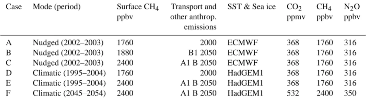
In order to assess the impact of 2000 to 2050 changes in emissions by each transport mode on the tropospheric chem-ical composition, six sets of experiments (Table 2) were performed for present, and future (A1B and B1 scenario)

Table 2. Set-up of the LMDz-INCA modelling experiments. The A to C experiments correspond to nudged simulations (2002–2003,

ECMWF meteorology) and the D to F experiments to 10-yrs climatic simulations (GCM mode). For each of these runs, “perturbation” runs have been performed, by applying a 5% emission reduction to each of the three transport modes separately (Cases A to C) and/or simultaneously (Cases D to F). The first and the first three years have been discarded as the spin-up of the model, for nudged and climatic runs, respectively.

Case Mode (period) Surface CH₄ Transport and SST & Sea ice CO₂ CH₄ N₂O ppbv other anthrop. ppmv ppbv ppbv emissions A Nudged (2002–2003) 1760 2000 ECMWF 368 1760 316 B Nudged (2002–2003) 1880 B1 2050 ECMWF 368 1760 316 C Nudged (2002–2003) 2400 A1 B 2050 ECMWF 368 1760 316 D Climatic (1995–2004) 1760 2000 HadGEM1 368 1760 316 E Climatic (1995–2004) 2400 A1 B 2050 HadGEM1 368 1760 316 F Climatic (2045–2054) 2400 A1 B 2050 HadGEM1 532 2400 350

emission datasets described in Table 1. Nudged runs over the 2002–2003 period, using the ECMWF operational winds and temperature fields, were performed, which allows an evaluation of the performance of the different global chem-istry models involved in QUANTIFY (Schnadt et al., 2010). The year 2002 was discarded to allow for the spin-up of the model and the year 2003 was analyzed. As described in Jourdain and Hauglustaine (2001), the Emanuel convection parameterization was used, which leads to a global annual NO production from lightning activity of about 5 Tg NOx -N, which is similar to other studies (e.g., Lee et al., 1997; Prather et al., 2001).

In addition to the base runs reported in Table 2, cor-responding 5% (and 100%) perturbed runs were also per-formed. To account for the corresponding changes in CH4 emissions, the CH4 concentrations were prescribed as sur-face boundary conditions in the INCA model, on the basis of time-varying tropospheric mean mixing ratio of methane provided by the ENSEMBLES project (Hewitt and Griggs, 2004). A monthly and latitudinal variability of CH4 sur-face concentrations, based on observations from the AGAGE database was applied to these averaged mean ratios to ac-count for the natural variability (J¨ockel et al., 2006). An ad-ditional set of unperturbed/perturbed B1 scenario was also simulated in order to assess the impact of possible mitigation options for aircraft, by reducing the NOxaircraft emissions according to ACARE (Advisory Council for Aeronautics Re-search in Europe; http://www.acare4europe.org/) targets for year 2050, as described in Table 3. These emission change experiments do not consider any climate change, which ef-fects are further analyzed through the climate change exper-iments, described in the following section.

3.3.2 Climate change experiments

Two 10 year periods (1995–2004 and 2045–2054) were sulated with the LMDz-INCA model in order to study the im-pact of climate change (Table 2). The first three years were discarded as the spin-up of the model and the 7 remaining years were averaged for each month of the year. Like the emissions change experiments, the impact of the transport emissions is assessed through a small perturbation approach (5% emission reduction). However, for computing sake, the perturbation is simultaneously applied to all the transport modes, rather than to each mode separately.

Firstly, the 2000 emissions were simulated in a present cli-mate (Case D). Then, for both 10 year periods, the chem-ical emissions were fixed at 2050 level, in order to iso-late the effect of climate change only (Cases E to F). The 2050 emissions from the A1B scenario were used. CO2, CH4 and N2O green house gas concentrations were fixed in the LMDz model to 368 ppmv, 1760 ppbv and 316 ppbv and to 532 ppmv, 2400 ppbv and 350 ppbv, for “present” (2000) and future (2050) climates, respectively, on the basis of IPCC (2001). Transient climate simulation outputs from the Hadley Centre Global Environmental Model version 1 (HadGEM1) were used for sea-surface temperatures and sea ice (Stott et al., 2006). A 10-year averaging has been per-formed for each month separately to drive the LMDz model, over the 1995–2004 and 2045–2054 periods.

The difference between D and E base runs gives an es-timate of the impact of 2000–2050 change in emissions in a present climate, whereas the impact of climate change is calculated from the difference between cases E and F. The E and F perturbed runs (5% reduction in transport emis-sions) provide an estimate of the impact of 2050 emissions by the transport sector in a present and future climate, re-spectively. Finally, the change between the two latter im-pacts gives an estimate of the effect of climate change on the

Table 3. Present 2000 and future (2050) global NOxemissions by aircraft (and all transport modes).

Year Scenario Traffic Demand Aircraft technology NOxin Tg(N) yr−1 description (all transports)

2000 Current Current 0.85 (14.1)

2050 A1B(i) GDP driven Moderate to good fuel efficiency, 3.33 (14.29) moderate NOximprovements

B1 GDP driven but intra-regional Good fuel efficiency 1.05 (6.6) growth decoupled from GDP improvements

B1 ACARE GDP driven but intra-regional Excellent fuel efficiency and 0.70 (6.2) growth decoupled from GDP NOximprovements: ACARE targets

achieved in 2020 and continuing improvements beyond 2020.

impact of emissions by the transport sector between 2000 and 2050. It must be emphasized here that the present (experi-ments A to E) and future (experiment F) climates are fixed using HadGEM1 simulation outputs, and therefore, that the changes in the tropospheric chemistry simulated in this study do not feedback on climate.

4 Results and discussion

4.1 Impact of present-day transport emissions on the global tropospheric chemistry

In this section, we assess the impact of present (2000) emissions by each of the three transport modes on tropo-spheric ozone from a 5% perturbation approach, based on our base run inventory (Table 1). The results are illustrated for July, which is the most documented month in the liter-ature. The ozone perturbations due to 2000 transport emis-sions (Case A) are shown in Fig. 1. The perturbation of the tropospheric ozone column by all transport emissions is char-acterized by a strong hemispheric difference, with maximum effects in the Northern Hemisphere. A maximum impact is simulated over Europe and the Central Atlantic, reaching up 5 DU for the 100% up-scaled perturbation (instead of 4.5 DU for LMDz-INCA preliminary simulations, Hoor et al., 2009). The zonal mean ozone mixing ratio perturbation shows a maximum of 7 ppbv in the upper troposphere/lower strato-sphere in the northern extra-tropics. At the surface, the total transport perturbation is also mainly concentrated over the Northern Hemisphere, with maxima of 8 ppbv over both land (over the eastern and western coasts of the US and over Ara-bia) and sea (Mediterranean Sea) regions. Due to titration effect (Eyring et al., 2007), a slight ozone decrease is pre-dicted under high NOxconditions over the North Sea.

Future changes in ozone production by the transport sec-tor will strongly depend on the respective contributions of the different transport modes (see for instance, Dahlmann

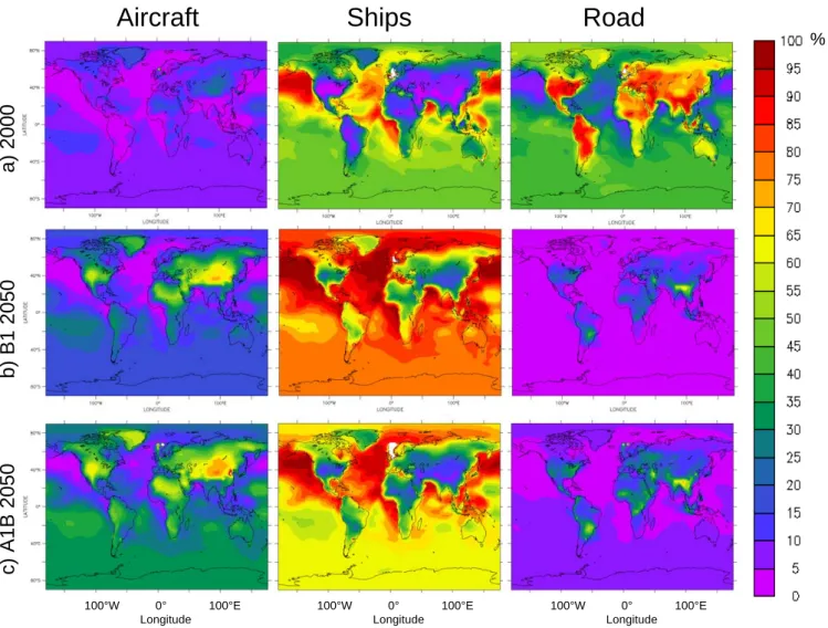
et al., 2009). Therefore, it is important in terms of mitiga-tion opmitiga-tions, to quantify the present and the future respec-tive contributions of each of them. Figures 2, 3 and 4 show the relative contribution of each transport modes to the total transport-induced perturbation of the ozone tropospheric col-umn, surface mixing ratio and zonal mean mixing ratio, re-spectively. The role of present-day road emissions is highly dominant in comparison to the two other modes. It reaches up 85% over Asia, 75% over the US and 70% over Europe for the tropospheric column perturbation (Fig. 2). The rela-tive contribution of road emissions to the ozone mixing ratio peaks in the free troposphere in both hemispheres, with a pronounced seasonal cycle in the northern extra-tropics, and a maximum in July. During summer, the boundary layer mix-ing and convective transport into the free troposphere of the road traffic emissions are more vigorous (Hoor et al., 2009). This explains the obtained seasonal cycle of the perturbation and why a high impact of road emissions is not only pre-dicted in the boundary layer over land, where it accounts for up to 95% of the total perturbation (Fig. 3), but also in the free troposphere (Fig. 4). Road traffic emissions account for up to 70% and 60% of the total zonal mean perturbation in the mid and northern high troposphere. North of 40◦_{S, the}

contribution of shipping emissions to the ozone column and to the zonal mean mixing ratio in the mid (<800 hPa) and upper troposphere is lower than for road traffic emissions (Fig. 4). In low troposphere, shipping emissions are the ma-jor perturbation in both hemispheres (i.e. >50% and >40% of the total transport perturbation on the ozone column and on the zonal mean mixing ratio, respectively), with a max-imum share of 60% at the equator. The impact is mainly located over marine regions, islands and coastal areas, where it represents up to 95% of the total transport-induced pertur-bation on the surface ozone mixing ratio (Fig. 3). Despite much lower emission levels than for ships and road traffic, NOx emitted by aviation also lead to a significant increase of ozone in the upper troposphere. This is due to higher

x 5

a. Zonal mean ozone (ppbv) c. Surface ozone (ppbv)

200 400 600 800 1000 200 400 600 800 1000 200 400 600 800 1000 200 400 600 800 1000 hPa

b.Tropospheric ozone column (DU)

100°W 0° 100°E Longitude 100°W 0° 100°E Longitude 80°S 40°S 0° 40°N 80°N Latitude

Fig. 1. Total (aircraft, shipping and road traffic) transport up-scaled (5% decrease effect × 20) perturbation in July for (a) zonal mean

ozone (1 ppbv), (b) tropospheric ozone column (1 DU), and (c) surface ozone (1 ppbv), due to 2000 (A experiment), 2050 B1 scenario (B experiment) and 2050 A1B scenario (C experiment) emissions (the solid line on plots a indicates the tropopause).

ozone production efficiency than for the two other modes. The LMDz-INCA results for QUANTIFY aircraft emissions (0.85 Tg(N) yr−1)are qualitatively and quantitatively close to those obtained for AERO2K emissions (0.67 Tg(N) yr−1). The maximum perturbation mainly lies from 250 to 350 hPa and 40◦ to 70◦N, which corresponds to the North Atlantic Flight Corridor. Maximum perturbations of 2.5 and 2.4 ppbv are respectively obtained in the UTLS of Northern Hemi-sphere, corresponding to 40% of the total transport pertur-bation in this area for July (Fig. 4). The impact in the lower troposphere (<10% in zonal mean; Fig. 4) and at the surface (<15% over most of the globe; Fig. 3) is low, except over Northern Asia, where it reaches up 30% of the total surface perturbation by the three transport modes.

Figure 5 shows the ozone perturbation to the combined emissions from the different transport sectors. As for Fig. 1, the 100% up-scaled perturbations are displayed to better al-low the comparison with Hoor et al. (2009). The perturba-tion ranges from 4% to 9% (Western Europe, Indian ocean, Southern Asia) and 10% (Mexico Gulf) for the ozone

col-umn, North of 20◦S in July (Fig. 5), and throughout the year (not shown). In the southern extra-tropics, the per-turbation is less than 5%. The relative perper-turbation to the zonal mean ozone ranges from 4% to 8% in the UTLS in the Northern Hemisphere, and up to 13% in the boundary layer. The perturbation in the Southern Hemisphere is about 4–5% in the low and middle troposphere (below 500 hPa) and of 2–3% above.

Hereafter, we compare our simulations results from a total removal of emissions from each transport mode (not shown) to previous studies using the same approach. As for our 5% road emission perturbation run, the total removal of the road traffic emissions in the LMDz-INCA model leads to a max-imum ozone perturbation in July, when they are responsible for an increase in the zonally averaged ozone of up to 7% in the boundary layer, 5% at 500 hPa and 4% at 300 hPa, in the Northern Hemisphere. These results are consistent with Niemeier et al. (2006) who reported very similar spa-tial patterns, and slightly higher perturbations (up to 10%, 6% and 5%, respectively). Matthes et al. (2007) results are

Aircraft

Ships

Road

a) 2000

c) A1B 2050

b) B1 2050

Fig. 2. Respective contribution (%) of each transport mode to the tropospheric ozone column change due to transport in July, for 2000

(A experiment) and 2050 (B1 and A1B scenarios; B and C experiments, respectively) emissions.

somewhat larger (up to 12%, 8% and 6%, respectively). As previously mentioned, both previous studies used similar to-tal road emissions for NOx, but higher amounts for CO and NMHC than in the present work. Removing all shipping emissions leads to a decrease in the near-surface zonal mean of up to 3.2 ppbv and 1.8 ppbv at northern mid-latitudes for July and annual zonal means, respectively. A relative contri-bution up to 5% (over Asia) and 50% (over the North Pacific) to the ozone column and surface ozone are calculated, re-spectively. These results are of the same order of magnitude than in Eyring et al. (2007): using 30% lower NOxemissions from shipping, this multi-model study reported an increase in near-surface annual and zonal mean O3up to 1.3 ppbv, rang-ing from 1.0 (LMDz-INCA) to 1.9 ppbv, accordrang-ing to the model. They obtained a maximum increase of about 12 ppbv (modeled ensemble mean) over the North Atlantic for July, whereas we obtain up to 8 ppbv and 9 ppbv over the Atlantic and Pacific oceans, respectively. Our results are closer to

Dalsoren et al. (2009), who calculated a contribution of the ship emissions of up to 5–6% to the tropospheric ozone col-umn (over the North Atlantic) and up to 40% to the surface ozone (over the North Pacific) for 2004 shipping emissions. As previously mentioned, Dalsoren et al. (2009) also used updated QUANTIFY emissions, but for 2004 (10% more NOxthan in 2000 QUANTIFY emissions). In both cases, the Northern Pacific is the most impacted region, whereas Eyring et al. (2007) obtained a much lower impact over the Pacific (<4 ppbv for the ensemble mean) compared to the Atlantic (up to 12 ppbv). This can explain the lower surface zonal mean O3 perturbation (1.3 ppbv against 1.8 ppbv) obtained in this previous study, which was shown to underestimate the shipping emissions over the Pacific ocean. We showed pre-viously that the impact of aircraft emissions on tropospheric ozone, as simulated by the LMDz-INCA model (5% per-turbation runs) using QUANTIFY and AERO2K emissions data and two different NOxlightning productions, are very

Aircraft

Ships

Road

a) 2000

c) A1B 2050

b) B1 2050

Fig. 3. Same as Fig. 2 for surface ozone mixing ratio.

similar, but located in the lower range of the perturbations reported in Hoor et al. (2009) for July. Our results for a total removal of QUANTIFY aircraft emissions lead to similar re-sults, with a maximum zonal-mean perturbation of 2.6 ppbv in the UTLS of Northern Hemisphere, which is significantly lower than the perturbation of 6 ppbv obtained by Gauss et al. (2006). One reason for such discrepancies is the strong dilution effect due to particularly high convection and mix-ing calculated by the LMDz-INCA model in summer, which induces lower ozone perturbations from aircraft and shipping compared to other models, and a maximum in spring.

4.2 2000 to 2050 changes in the impact of transport emissions

In this section, we describe the impact of the future changes in anthropogenic emissions on the role of the transport sector on the global tropospheric chemistry. The simulations have been performed for two different scenarios (Table 2). As previously, the 100% up-scaled perturbations are shown (see

Sect. 3.2). Except where stated, the results in this section are mainly discussed in terms of 2000 to 2050 relative change in the transport-induced ozone perturbation rather than in terms of absolute perturbation. The impact of emissions from each transport mode, and from all transport emissions are firstly reported. The sensitivity of the results to possible mitigation options is then discussed.

4.2.1 A1B and B1 emission scenarios

Based on the QUANTIFY future emissions, we assume a high reduction of road emissions, and a moderate (B1 sce-nario) to high (A1B scesce-nario) increase of ship and aircraft emissions in 2050. As a consequence, the contribution of road traffic to the O3 column perturbation drastically de-creases in 2050, accounting for less than 15% of the total transport perturbation over most of the globe, for both sce-narios (Fig. 2). Ship emissions become the predominant contribution to the O3 column perturbation in the South-ern Hemisphere, especially for the B1 scenario, for which

Aircraft

Ships

Road

a) 2000

c) A1B 2050

b) B1 2050

Fig. 4. Same as Fig. 2 for zonal mean ozone mixing ratio. The solid line indicates the tropopause.

it contributes up to 85% to the overall perturbation (Indone-sia). Ships also have a predominant contribution in the lower troposphere in the Northern Hemisphere (Fig. 4). Their in-fluence remains mainly located over marine regions, whereas aircraft have the strongest impact on ozone in the continen-tal boundary layer (Fig. 3). Nevertheless, in the case of the B1 scenario, the impact of shipping on surface ozone extends more inside the continents, because of the synoptic transport of ozone and its precursors inland. The surface ozone pertur-bation due to ship emissions in the most affected coastal re-gions increases from about 2 ppbv in 2000 to 3 ppbv. In both future scenarios, subsonic aviation becomes the major ozone perturbation in the Northern Hemisphere, by contributing up to 70% and 75% to the total transport perturbation over the US, and up to 80% and 85% over continental Asia, for B1 and A1B scenarios, respectively (Fig. 2).

In the case of the B1 scenario, the decreased transport emissions lead to a significant reduction (by roughly 50%) of the ozone perturbation throughout the troposphere in 2050 (Figs. 1 and 5). At the surface, an even more

pro-nounced decrease of the perturbation is simulated over land, due to the drastic reduction in road emissions. The to-tal (up-scaled) surface ozone perturbation over Western Eu-rope drops from 6 ppbv to less than 2 ppbv (Fig. 1c). For the same reason, the combined impact of traffic decreases over the oceans, despite a slight increase in ship emissions (from 4.39 to 5.05 Tg(N) yr−1). Despite similar total NOx transport emission in 2050 compared to 2000 (i.e., 14.3 against 14.1 Tg(N) yr−1), the A1B scenario leads to an in-crease of the impact of transport on ozone by up to +30% and +50% in the Northern and Southern Hemispheres, re-spectively (Figs. 1 and 5). The increase is even more pro-nounced in the UTLS region in the Northern Hemisphere. This is mainly due to a high increase in aircraft emissions (from 0.85 to 3.3 Tg(N) yr−1), and to their high ozone pro-duction efficiency. In the lower troposphere, in the Northern Hemisphere, the relative perturbation increases by 2050 ac-cording to scenario A1B, but to a lesser extent than in the up-per troposphere, and mainly at high latitudes (above 50◦_N).

a) 2000

c) A1B 2050

b) B1 2050

Tropospheric ozone column

Zonal mean ozone

% 200 400 600 800 1000 hPa 200 400 600 800 1000 hPa 200 400 600 800 1000 hPa 80°S 40°S 0° 40°N 80°N Latitude 100°W 0° 100°E Longitude

Fig. 5. Up-scaled perturbations (in %) in the ozone tropospheric column (left) and in zonal mean ozone mixing ratio (right) due to all

transport modes, obtained for July for 2000 (A experiment) and 2050 (B1 and A1B scenario, i.e., B and C experiments) emissions.

4.2.2 B1 ACARE mitigation

In order to assess the efficiency of possible aircraft emission reduction strategy, the B1 ACARE scenario was simulated for 2050. It corresponds to B1 emission scenario, but with a reduction of the aircraft emissions due to the implementation of ACARE targets (Table 3). It is characterized by low NOx global aircraft emissions (lower than for 2000), and can be seen as a more restricting but technically feasible scenario. The induced ozone perturbation for this scenario is illustrated and compared to 2000 and B1 2050 perturbations in Fig. 6. A 5% perturbation of aircraft emissions leads to a perturba-tion of less than 0.10% of the zonal mean ozone background of the upper troposphere of Northern Hemisphere, instead of up to 0.12 % and 0.14% for 2000 and B1 2050 emissions, respectively (Fig. 6a). The ozone column perturbations show a decrease of 25% to 36% of the impact of aviation

com-pared to B1 2050 (not shown). Whereas for B1 scenario, the aircraft impact increases over most of the globe from 2000 to 2050, the B1 ACARE scenario leads to an increase in the Southern Hemisphere (by up +30%), but a decrease in the Northern Hemisphere, by down to −30% (Fig. 6b). Never-theless, aviation would still be the major transport contrib-utor to the ozone perturbation in the Northern Hemisphere in 2050, by contributing by up to 70% to the total transport perturbation on the O3column (not shown).

Figure 7a shows the sensitivity of the global ozone burden to each transport mode, for 2000, 2025 and 2050 emissions. The predominant perturbation mode shifts from road to air-craft (A1 scenario) or shipping (B1 scenario) from 2000 to 2050. This shift is due to changes in the respective emis-sion amounts, whereas the ozone production efficiency (O3 molecule per NOxmolecule emitted) of each transport sector is not highly modified (Fig. 7b). In agreement with previous

a. Up-scaled ozone background perturbation (%) due to aircraft emissions (July)

2000 2050 - B1 scenario 2050 - B1 ACARE scenario

2.8 2.4 2.0 1.6 1.2 0.8 0.4 0.0 80°S 40°S 0° 40°N 80°N Latitude 80°S 40°S 0° 40°N 80°N Latitude 80°S 40°S 0° 40°N 80°N Latitude 200 400 600 800 1000 hPa

b. 2000 to 2050 change (%) in the ozone perturbation due to aircraft emissions (July)

100 80 60 40 20 0 -20 -40 B1 scenario B1 ACARE scenario 80°S 40°S 0° 40°N 80°N Latitude 100°W 0° 100°E Longitude 80°S 40°S 0° 40°N 80°N Latitude 100°W 0° 100°E Longitude 160 140 120 100 80 60 40 20 0 -20 -40 160 140 120 100 80 60 40 20 0 -20 -40 200 400 600 800 1000 hPa 200 400 600 800 1000 hPa 100 80 60 40 20 0 -20 -40

2000 2050 - B1 scenario 2050 - B1 ACARE scenario

2.8 2.4 2.0 1.6 1.2 0.8 0.4 0.0 80°S 40°S 0° 40°N 80°N Latitude 80°S 40°S 0° 40°N 80°N Latitude 80°S 40°S 0° 40°N 80°N Latitude 200 400 600 800 1000 hPa

b. 2000 to 2050 change (%) in the ozone perturbation due to aircraft emissions (July)

100 80 60 40 20 0 -20 -40 B1 scenario B1 ACARE scenario 80°S 40°S 0° 40°N 80°N Latitude 100°W 0° 100°E Longitude 80°S 40°S 0° 40°N 80°N Latitude 100°W 0° 100°E Longitude 160 140 120 100 80 60 40 20 0 -20 -40 160 140 120 100 80 60 40 20 0 -20 -40 200 400 600 800 1000 hPa 200 400 600 800 1000 hPa 100 80 60 40 20 0 -20 -40

Fig. 6. (a) Perturbations in zonal mean ozone mixing ratio (in %) due to aircraft emissions, for July from 2000 (left), 2050 B1 (middle)

and 2050 B1 ACARE (right) emissions; (b) 2000–2050 changes (%) in the O3tropospheric column and zonal mean ozone perturbations by aircraft emissions for B1 scenario, and (c) B1 ACARE scenario.

studies (e.g., Hauglustaine et al., 2005; Gauss et al., 2006; Dahlmann et al., 2009; Hoor et al., 2009), aircraft NOx emis-sions show an ozone production efficiency about three times higher than road traffic and shipping, because they are emit-ted directly into the UTLS, where they lead to larger and more persistent perturbations compared to the Earth’s sur-face. The shipping emissions, which largely occur in low polluted environments, have the highest net chemical pro-duction per NOxmolecule (Fig. 7c).

4.3 Influence of climate change

In this part, we present the impact of transport emissions, in the context of climate changes for the A1B 2050 emission scenario. The effect of climate change on the future meteo-rological and chemical states of the troposphere is first pre-sented. It is compared to available published results, which mainly concerned scenario A2 and year 2100. The innovative investigation of the changes in the transport-induced ozone perturbation due to climate change is then presented.

0 2 4 6 8 10 12 14 1 2 3

Air - B1 Road - B1 Ship - B1

Air - A1B Road -A1B Ship - A1B

0 20 40 60 80 100 120 2000 2025 2050 Air - B1 Road - B1 Ship - B1 Air - A1B Road -A1B Ship - A1B

2,0 2,2 2,4 2,6 2,8 3,0 3,2 3,4 3,6 3,8 4,0 2000 2025 2050 Air - B1 Road - B1 Ship - B1 Air - A1B Road -A1B Ship - A1B

0,0 0,2 0,4 0,6 0,8 1,0 1,2 1,4 2000 2025 2050 Air - B1 Road - B1 Ship - B1 Air - A1B Road -A1B Ship - A1B

a. Perturbation of the global ozone burden

Tg O3

b. Perturbation of the global ozone burden

Mol. O3/emitted Mol. NOx-N.yr-1

c. Perturbation of the global ozone chemical net production

Tg O3.yr-1

d. Perturbation of the global ozone chemical net production

Mol. O3/emitted Mol. NOx-N

2000 2025 2050

2000 2025 2050

2000 2025 2050

2000 2025 2050

Fig. 7. Perturbation of the global ozone burden (a, b) and the global ozone chemical net production (c, d) due to 2000, 2025 and 2050

emissions from aircraft, road traffic and shipping. Both the absolute (left) and the relative (mol. O3 per mol. of emitted NOx; right) perturbations are presented.

4.3.1 Change in global climate and tropospheric chemical composition

The 2000–2050 climate change and its impacts on the back-ground chemical composition of the troposphere are based on the differences between E and F simulations (Table 2).

The change in the global mean annual surface temperature (+1.3◦C) as simulated by the LMDz-INCA model between

the two time-slice periods is consistent with the last IPCC re-sults (Meehl et al., 2007), which reported a 2000–2050 sur-face warming of +1.4◦C for A1B emission scenario, from an ensemble of 21 models. Surface temperature changes less than 4◦C are predicted in annual mean over most of the globe. A similar change is also generally predicted for Jan-uary and July (not shown), but reaching locally up to 9◦_C

(e.g., over the US and Eastern Russia). The zonal mean temperature increases by up to 2.5◦C throughout the tropo-sphere in July. Lower changes are obtained in January South to 40◦N, but higher ones more North (Fig. 8a). An associ-ated increase in water vapor is obtained in most of the tropo-sphere, reaching up to +60% in zonal mean in the UTLS re-gion (Fig. 8b). These changes in temperature and water vapor are consistent with previous studies. For instance, Brasseur

et al. (2006) predicted similar, but stronger changes (up to 150% for the water vapor) by July 2100 for the more pes-simistic A2 scenario, using ECHAM5/OM-1 model. The 2000–2050 changes in precipitation rate (not shown) simu-lated in our study also show similar general trends (decrease in tropical Atlantic and increase in tropical Pacific) compared to the 2000–2100 precipitation change simulated by Brasseur et al. (2006) for A2 scenario. As a result of enhanced water vapour, a decrease in future global ozone burden is generally predicted, since more water vapor leads to more ozone loss through O1(D) reaction with H2O (Stevenson et al., 2006). However, both positive and negative ozone changes are re-ported according to the altitude, the season, the model, the reference year or the scenario (e.g., Hauglustaine et al., 2005; Murazaki and Hess, 2006; Wu et al., 2008). Figure 9a shows the calculated 2000–2050 changes in the ozone, NOxand CO zonal means for scenario A1B, in January and July. We ob-tain similar spatial patterns, but logically lower magnitude of changes compared to the 2000–2100 changes illustrated in Brasseur et al. (2006) and Hauglustaine et al. (2005), for the more pessimist A2 scenario. A decrease of the ozone mix-ing ratio reachmix-ing up 10% is predicted in both hemispheres. Between 900 hPa to 400 hPa, this net decrease is associated

+ 8.0 + 6.0 + 4.0 + 3.5 + 3.0 + 2.5 + 2.0 + 1.5 + 1.0 + 0.5 0.0 - 0.5 - 1.0 - 1.5 - 2.0 + 150 + 100 + 50 + 40 + 30 + 20 + 10 + 5.0 0.0 - 5.0 July January

a. Change in zonal mean temperature (°C)

b. Change in water vapour (%)

July January 80°S 40°S 0° 40°N 80°N Latitude 80°S 40°S 0° 40°N 80°N Latitude 80°S 40°S 0° 40°N 80°N Latitude 80°S 40°S 0° 40°N 80°N Latitude 200 400 600 800 1000 hPa 200 400 600 800 1000 hPa

Fig. 8. Future (2050) change in zonal mean temperature (degrees) and water vapour (%), for July (left) and January (right) conditions (A1B

emission scenario).

with an increase in the chemical loss of ozone twice higher than the increase in the chemical production (not shown). In addition to these processes, the decrease of ozone also pre-dicted in the lower troposphere (below 800 mb) around 20◦N and 20◦S in July and January respectively, is due to a shorter lifetime of ozone and peroxyacetylnitrate (PAN) at warmer temperatures (Wang et al., 1998; Hauglustaine et al., 2005; Brasseur et al., 2006; Wu et al., 2008). This process would allow explaining the associated increase in NOx concentra-tions (Fig. 9b) and the strong positive change in ozone chem-ical net production at these altitudes (not shown). According to the latter previous studies, the larger ozone decrease (up to 6%–10%) predicted in the upper troposphere (∼300 hPa) could also reflect the elevation of the tropopause height due to climate change (see also Collins et al., 2003).

In a warmer climate, the hydrological cycle is more active and the convection enhanced. Such an increase in convec-tion and the related lightning NOx production were shown to have a strong impact on NOxbackground concentrations, and thus on the magnitude of the anthropogenic perturbations

on upper tropospheric ozone. On one hand, it was shown to lead to a higher production of lightning NOx, and thus to an increase in NOxand ozone concentrations, especially in the tropics (Hauglustaine et al., 2005; Zhao et al., 2009). On the other hand, the stronger vertical mixing due to convec-tion reduces the NOxbackground concentrations in the up-per troposphere of extra-tropical regions, and consequently to increase the ozone production efficiency of aircraft NOx emissions. Results from our simulations show an increase by up to 25% in NOxbackground concentrations in the up-per troposphere over the inter-tropical region (Fig. 9b). This climate-induced increase is due to the NOx production by lightning, which is shown to increase by 7.3% at global scale because of enhanced convection, from 4.67 to 4.84 Tg NOx -N. As a consequence, the zonal mean ozone concentration increases by up to 4% in the UTLS in this region. Inversely, in the extra-tropical latitudes, a decrease in NOxbackground concentrations by more than 25% is predicted in the mid and upper tropospheres in July, and throughout the troposphere in January.

Figure 9

Impact of climate change on NO

(%), O3 (%) and CO (ppb

)

+100 +50 +25 +5 +2 0 -2 -5 -25 -50 -100

b

. Change in zonal mean NO

(%)

+ 8 + 6 + 4 + 2 0 - 2 - 4 - 6 - 8 - 10 - 12 - 14

a

. Change in zonal mean O

(%)

July

January

July

January

Fig. 9. Future change in O3(%) and NOx(%) zonal mean mixing ratio, for July (left) and January (right) conditions (A1B emission scenario).

4.3.2 Change in the impact of transport on tropospheric chemistry

In this section, we assess the effect of climate change on the impact of future transport emissions on tropospheric ozone, from present (Case E) and future (Case F) base and per-turbation runs (Table 4). As done in the previous section, the transport perturbations were assessed by a 5% perturba-tion of emissions, subsequently up-scaled to 100%. While this approach was shown to under-estimate by 8% the global transport-induced ozone perturbation, it does not signifi-cantly affect the evaluation of its changes due to climate change, since it was applied to both present and future cli-mates. The simulated impact of 2000 (Fig. 10a) and A1B 2050 (Fig. 10b) transport emissions on the ozone column in a present climate are consistent with the results previously obtained from 2003 meteorological runs (Fig. 1b). Simi-lar spatial patterns but slightly lower perturbations are ob-tained for these climatic runs. The general patterns of the impact of A1B 2050 transport emissions on the ozone col-umn are very similar in the future (Fig. 10c) and present (Fig. 10b) climate. In both cases, an increase in the ozone column is predicted, with (up-scaled) maxima of +5.0 DU (January) and +5.5 DU (July) in the Northern Hemisphere.

In July, the most impacted area (>4.0 DU) mainly extends from the Eastern US to Eastern Europe, and also includes a large part of the Mediterranean region. In January, Asia and the North Pacific Ocean also experience an increase by up to +5.0 DU (present climate) and +4.5 DU (future climate). The perturbation of the ozone zonal mean mixing ratio (not shown) reaches +9 (and +9) ppbv in the upper troposphere of the Northern Hemisphere in July, and +7.5 (and +8.0) ppbv in January, for the present (and future) climates. These results are consistent with the nudged simulations results, which showed that this high impact of 2050 transport emissions in the upper troposphere in the Northern Hemisphere was due for a large part to the aircraft emissions and their high ozone production efficiency (Figs. 4 and 5).

While very similar global patterns for the impact of trans-port emissions on ozone are predicted with and without the climate change, significant positive or negative climate-induced changes are simulated according to the region, alti-tude and season. An increase of up to +0.6 DU is simulated in January in both northern (North Pacific) and southern (West coast of South-America) hemispheres (Fig. 1a). In July, the climate change enhances the effect of transport emissions in the already most impacted zone, by up to 0.4 DU (i.e, by +10%) in the Gulf of Mexico (Fig. 11b). In Western Europe,

Table 4. Impact of changes in emissions and in climate, on the global tropospheric chemistry. “O3prod.”, “O3loss” and “O3net” refer to the O3chemical production, O3chemical loss and O3chemical net production, respectively. The r subscript letter refers to 5% reduction of transport emissions. See Table 2 for the definition of the D, E and F experiments.

Changes in the global tropospheric NOx OH CH4 O3 O3 O3 O3 Case chemistry due to: light. lifetime burden prod. loss net

2000 to 2050 emission change 0,0% −1.3% +3.3% +10.1% +12.4% +13.8% +8.0% (E–D)/D 2000 to 2050 climate change 7,3% +2.3% −4.7% −1.2% +2.4% +3.9% −2.7% (F–E)/E Emissions and climate changes 7.3% +1.0% −1.6% +8.8% +15.0% +18.3% +5.1% (F–D)/D 2000 transport emissions in a present climate 0,0% +5.4% −6.5% +5.4% +8.8% +7.8% +12.7% [(D–Dr) · 20]/D 2050 transport emissions in a present climate 0.0% +9.0% −9.7% +6.6% +9.6% +8.7% +12.2% [(E–Er) · 20]/E 2050 transport emissions in a future climate 0,0% +9.0% −9.7% +6.6% +9.6% +8.7% +12.5% [(F–Fr) · 20]/F

Table 5. Impact of changes in emissions and in climate on the perturbation of the global tropospheric chemistry by the transport emissions.

“O₃prod.”, “O₃loss” and “O₃net” refer to the O₃chemical production, O₃chemical loss and O₃chemical net production, respectively. The r subscript letter refers to 5% reduction of transport emissions. See Table 2 for the definition of the D, E and F experiments.

Change in the transport-induced OH CH4 O3 O3 O3 O3 Case perturbations due to: lifetime burden prod. loss net

2000 to 2050 emission change +65% +53% +37% +22% 31% +4% [(E–Er)]–(D–Dr)]/(D–Dr) 2000 to 2050 climate change +1.9% −4.8% −1.6% +2.7% +3.9% +0.1% [(F–Fr)–(E–Er)]/(E–Er) 2000 to 2050 emissions and climate changes +68% +46% +35% +25% +36% +4% [(F–Fr)–(D–Dr)]/(D–Dr)

an increase reaching up 0.3 DU (July) and 0.4 DU (January) is obtained, corresponding to +6% and +12%, respectively. Decreases of the same order of magnitude are also predicted in SE Asia in January (−0.6 DU corresponding to −20%), but also over Africa and in the North Pacific in July (−0.5 DU, i.e., −16%). The changes in the zonal mean mixing ratio (Fig. 11c) show an increase throughout the troposphere north to 20◦_{N, which reaches up to 0.5 ppbv at the tropopause}

level, i.e. 8% of the impact of transport (Fig. 11c). This in-crease clearly results from the dein-crease in NOxbackground concentrations predicted throughout the troposphere in Jan-uary, that leads to an enhanced ozone production efficiency of NOxemissions, and notably of aircraft emissions. In July, a similar increase is obtained in the upper troposphere for the same reasons, whereas the impact of transport emissions on ozone decreases by 0.5 ppbv (−8%) in the low troposphere (around 800 hPa) of Northern Hemisphere (Fig. 11d). As for the ozone background levels (Fig. 9a), this decrease is re-lated to the increase in the water vapor content and the as-sociated decrease in the net ozone chemical production. In the Southern Hemisphere, except for the southern polar re-gion (July), and around 20◦_{S latitude (January), a decrease}

of the impact of the transport emission is generally predicted, which reaches −0.6 ppbv in the upper troposphere of the inter-tropical region. Figure 12 shows the seasonality of the zonal mean ozone column perturbation as simulated by LMDz-INCA for the present and future climates. In both

cases, the minimum and maximum transport-induced pertur-bations are calculated for summer and winter, respectively. A more pronounced perturbation change is calculated for win-ter than for summer. The main reason for this is that the effect of aircraft emissions on the ozone perturbation, which is ap-proximately half as large during January compared to July, becomes highly dominant in future according to the A1B fu-ture scenario.

The global effects of climate and emissions changes on the ozone background and on the transport-induced ozone are summarized in Table 4 and Table 5, respectively. Changes in the OH concentration and CH4lifetime are also reported. The results show that the changes in all anthropogenic emis-sions increase the global tropospheric O3 burden by about 10%, whereas the climate change leads to a decrease of 1.2%. This decrease is due to an increased ozone chemical loss (+3.9%) which dominates the increase in the ozone chemical production (+2.4%), as discussed in section 4.31. As a con-sequence of both emissions and climate changes, the ozone burden increases by 8.8% in annual mean (Table 4). The at-mospheric chemical perturbations from transport emissions are affected by climate change in a similar magnitude as the background chemistry (Table 5). The transport-induced ozone production and destruction rates are increased by 2.7% and 3.9%, respectively. As result, the perturbation of the ozone burden due to transport emissions decreases by 1.6% because of climate change. In comparison, the changes in