Modeling Fine-Scale Geological
Heterogeneity—Examples of Sand Lenses in Tills
by Timo Christian Kessler
1,2, Alessandro Comunian
3, Fabio Oriani
4, Philippe Renard
4, Bertel Nilsson
2, Knud Erik
Klint
2, and Poul Løgstrup Bjerg
5Abstract
Sand lenses at various spatial scales are recognized to add heterogeneity to glacial sediments. They have high hydraulic conductivities relative to the surrounding till matrix and may affect the advective transport of water and contaminants in clayey till settings. Sand lenses were investigated on till outcrops producing binary images of geological cross-sections capturing the size, shape and distribution of individual features. Sand lenses occur as elongated, anisotropic geobodies that vary in size and extent. Besides, sand lenses show strong non-stationary patterns on section images that hamper subsequent simulation. Transition probability (TP) and multiple-point statistics (MPS) were employed to simulate sand lens heterogeneity. We used one cross-section to parameterize the spatial correlation and a second, parallel section as a reference: it allowed testing the quality of the simulations as a function of the amount of conditioning data under realistic conditions. The performance of the simulations was evaluated on the faithful reproduction of the specific geological structure caused by sand lenses. Multiple-point statistics offer a better reproduction of sand lens geometry. However, two-dimensional training images acquired by outcrop mapping are of limited use to generate three-dimensional realizations with MPS. One can use a technique that consists in splitting the 3D domain into a set of slices in various directions that are sequentially simulated and reassembled into a 3D block. The identification of flow paths through a network of elongated sand lenses and the impact on the equivalent permeability in tills are essential to perform solute transport modeling in the low-permeability sediments.
Introduction
In large areas of Scandinavia and North America the superficial geology comprises glacial sediments with low hydraulic permeability (Houmark-Nielsen 2003). These 1Technical University of Denmark, DTU Environment, Miljøvej 113, 2800 Kgs. Lyngby, Denmark.
2Geological Survey of Denmark and Greenland, Øster Voldgade 10, 1350 Copenhagen, Denmark.
3University of New South Wales, National Centre for Groundwater Research and Training, 2052 UNSW, Sydney, Australia. 4University of Neuchˆatel, Centre for Hydrogeology and Geothermics, Rue Emile-Argand 11, 2000 Neuchˆatel, Switzerland.
5Corresponding author: Technical University of Denmark, DTU Environment, Miljøvej 113, 2800 Kgs. Lyngby, Denmark. +4545251615; fax: +4545932850; [email protected]
clayey tills are typically riddled with sub-vertical fractures and horizontally oriented lenses of sand and gravel (McKay and Fredericia 1995; Klint 2001; Kessler et al. 2012). Depending on the size, frequency, and spacing, sand lenses are suspected to create channel networks within the till matrix and to influence the subsurface hydraulic conductivity field (Harrington et al. 2007). This is particularly true for geological settings where matrix flow is diffusion limiting and preferential flow controls subsurface transport (McKay et al. 1993; Broholm et al. 2000; Nilsson et al. 2001; Jørgensen et al. 2002; Eaton 2006; Harrar et al. 2007). The demand for realistic transport models in such settings on local scale for contaminated sites requires high-resolution geological data including heterogeneity at decimeter scale and below. Sand lenses are the result of glacial deposition and deformation. Material evolves from sub- or proglacial fluvial/lacustrine sedimentation (Sharpe and Cowan 1990;
Sadolin et al. 1997; Eyles 2006) or as debris flow near the glacier margin (Dreimanis 1993; Bertran and Texier 1999; Phillips 2006). Depending on the deposition regime, the sediments have different characteristics in terms of com-position, extent and, shape. Detailed descriptions of sand lens types occurring in tills and a classification scheme were published by Kessler et al. (2012). Most common are small pockets and stringers that are embedded in the matrix and occur in high numbers and short spacing. They are lense-shaped features at the scale of centimeters to decimeters. They have long tailing from the end of the pocket evidencing shear deformation within the till. They can reach thicknesses of 10 to 50 cm (Kessler et al. 2012). The focus of this study is to examine the forms, the spa-tial relation, the connectivity, and the importance for the hydraulic conductivity field of these types of sand lenses. Noninvasive geophysical methods have been used to characterize and record lithofacies distribution at the aquifer and even site scale (Huggenberger et al. 1994; Asprion and Aigner 1997; Bayer et al. 2011). In clayey soils with fine-scale heterogeneity these methods have shown limited applicability in larger depths (Kilner et al. 2005; Cuthbert et al. 2009). Analog studies on vertical outcrops are more useful to examine complex facies architecture and spatial variability of geological features in two dimensions (Falivene et al. 2006; Bayer et al. 2011; Comunian et al. 2011b). Sand lenses in tills show irregular geometries and typically concentrate in depths larger than 5 to 10 m below ground surface (b.g.s.) (Gerber et al. 2001; Hendry et al. 2004). Mapping exercises for this type of heterogeneity need to describe the spatial distribution, but also anisotropic shapes, variable sizes, and spacing between single lenses (Kessler et al. 2012). The specific framework of sand lenses in tills is not suited for a combined approach using both, geophysical data and analog observations for cross-evaluation. Such an approach was presented for example for a sandy-gravelly fluvial aquifer system by Bayer et al. (2011). The expected lower resolution of geophysical data compared to outcrop data made further considerations redundant.
The analysis of spatial variability in geological set-tings is one of the core disciplines of geostatistics (Deutsch and Journel 1992; Goovaerts 1999; Webster and Oliver 2007). Measures of spatial correlation inform about the configuration and architecture of facies and are used to predict realizations of geological variables at unsampled locations. The main limitation of variogram-or covariance-based methods is the lack of geological structure being accounted for. Nonetheless, sequential indicator statistics (SIS) were used to model multi-categorical geological systems (e.g., Sminchak et al. 1996; Falivene et al. 2006; dell’Arciprete et al. 2012). Klise et al. (2009) applied the method to a complex two-category system and showed that SIS does not repli-cate connectivity patterns, even if highly conditioned. Transition probability-based methods (TP) were employed to model facies distribution where indirect geological knowledge was available, for example in alluvial aquifer systems (Carle 1996; Carle et al. 1998; Weissmann and
Fogg 1999). Fogg et al. (1998) and Lee et al. (2007) point out that TP models are advantageous compared to covariance-based models because they capture cross-correlations between facies (juxtapositioning tendencies). Multiple-point statistics (MPS) includes higher-order statistics yielding enhanced capabilities in simulating complex spatial structures (Strebelle 2002; Liu 2006; Hu and Chugunova 2008). MPS was used for a number of synthetic cases (Feyen and Caers 2006; Arpat and Caers 2007) as well as field applications (e.g., Huysmans and Dassargues 2009; Comunian et al. 2011b). Most studies apply MPS to field data where training images (TIs) were constructed from outcrop observations at a scale of tens of meters. Generally, stochastic modeling of geology has emphasized in the past on modeling facies distribution and architecture of multicategorical settings with rather crude geological knowledge. Less attention was paid to reproduce geometries of specific geological configurations at small scale. Bastante et al. (2008) applied the MPS method to such a scenario modeling slate deposits, but the dataset is based on borehole logs and therefore less detailed compared to outcrop data.
The aim of this study is firstly, to analyze geometry, structure, and variability of fine-scale geological hetero-geneity in clayey tills. Secondly, to simulate the geometry and distribution of sand lenses, and, thirdly, to evalu-ate whether sand lenses can creevalu-ate connected channel networks that affect the bulk hydraulic conductivity in clayey tills. Sand lenses were hereby treated as geologi-cal features embedded within a homogeneous till matrix. This allows us to consider only two lithofacies for data collection and subsequent simulation. Simulations were done with TP and MPS algorithms to test the appropri-ateness for the collected datasets. Focus was turned to the capability to reproduce complex structures and nonsta-tionary section images. Channel networks were assessed with calculations of connectivity functions and equivalent permeability. The overall research questions we address is how useful are high-resolution, two-dimensional (2D) datasets to simulate complex structures at the decimeter scale and how much does fine-scale heterogeneity matter for transport in till settings.
Methodology
Outcrop Data Collection
Sand lenses were mapped on vertical profiles at a clayey till outcrop in the Kallerup gravel pit. The excavation is located in the Eastern part of Denmark (Figure 1) and exposes a vertical sequence of till units sedimented during consecutive ice advances. A detailed description of the geology and till stratigraphy including the associated sand lens occurrences is presented by Kessler et al. (2012). The investigated till profile is about 12-m deep and 24-m long. Sand pockets and sand stringers occur in high numbers in a basal till unit of 3-m thickness in about 10-m depth.
A rectangular block of 6 by 6 m lengths and 2 m height was chosen as a sample volume (Figure 5). The
Kallerup gravel pit 100 km Jutland Zealand Funen Ice movement direction
Main stationary ice line East Jutland ice-border line Bælthav ice margin
Figure 1. Location of the Kallerup site in the Eastern part of Denmark, where sand lenses were mapped on till outcrops. The dashed gray lines indicate three major glaciation extensions from the Northeast or Main Advance according to Houmark-Nielsen (2007). The figure is modified from Kessler et al. (2012).
outer boundaries of the block were excavated and scraped off. It offers four equally distant cross sections at the size of 6 m by 2 m, both parallel and perpendicular to the ice-movement direction (Figure 5). The combination of different-angled cross sections reveals potential horizontal anisotropy and yields a quasi-three-dimensional (3D) representation of the geology. Anisotropy occurs if mean lengths differ with direction (Carle and Fogg 1996). Most sand lenses have characteristic lengths of half a meter, but elongated sand sheets may reach horizontal extents of several meters. Each measured cross section contains at least 20 individual sand lenses. Thus, we considered the dataset suitable for a statistical study and to justify a resolution in the order of centimeters. It is crucial to choose the appropriate scale for the cross sections to capture the details of small sand stringers, but at the same time to also surround larger deposits. The sections cover the various shapes, sizes, and related geometric parameters of individual lenses, given the lenses do not outreach the extent of the section. Most geometric parameters can be determined in the field using tape-measure and geological compass (Figure 2).
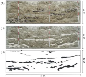
Two-dimensional sections further provide information on the spatial variability. The configuration of lenses in space was recorded using photographic mapping tech-niques (Fraser and Cobb 1982; Jussel et al. 1994). Pic-tures were taken from the cross sections and the limits of the sand lenses were drawn by hand onto the image (Figure 2). The sand facies have different coloring com-pared to the surrounding till and distinct contacts enabled precise reproductions of shapes in the range of few mm to 2 cm. The image was then converted into a numeri-cal dataset for processing and analysis. The geology was categorized into two facies, sand lenses and the surround-ing clayey matrix, the latter besurround-ing chosen as background category. When translating the digital datasets into binary files the resolution can be chosen according to the desired level of detail. This type of data collection capturing not only vertical successions of geological facies (like lithological interpretations of borehole logs) but providing structural information, further allows the data to be used
(A) (B) (C) 6 m m 2 m 2 m 2 Length
ThicknessDip angle Deformation
structures
Figure 2. Outline of the mapping procedure of sand lenses on vertical till cross sections: (A) scraped section of the investigated till profile; (B) observed sand lenses drawn on the picture; and (C) conversion of the section into binary data with the two categories clay (white) and sand (black).
as TIs for stochastic simulation algorithms, for example, MPS.
TP and MPS Model Tools
The two selected simulation methods (TP and MPS) are parameterized in different ways. The TP method deter-mines spatial correlation with one-dimensional Markov chains in each direction. In the case of two categories, cross-correlations are dispensable and the variability is parameterized only with categorical proportions and mean lengths of each lithofacies (Carle and Fogg 1996). These attributes are derived from transiograms that display the auto- and cross-transitions at each lag distance h. Tran-siograms are equivalent to traditional variograms, showing the TP instead of the variances of a geological variable (Figure 3). The transitions depict the probability that the geological category does or does not change from one point in space to another (Carle 1999). The high-resolution datasets from the section images allow simulating the data at lag distances of 1 cm resulting in a precise fit of the Markov models. The Markov chains are calculated for the training sections and are subsequently used for the simulation of parallel target sections. The reference pro-portions are directly calculated from the digital section images. The TP algorithm can be equally employed for 2D and 3D simulations because the orientation of the cross sections allowed computing at least one transiogram for each direction.
MPS use TIs to study spatial patterns and to implement them in a sequential simulation procedure. The method is expected to show remarkable advantages regarding the reproduction of single sand lenses because 2D geometries are recognized by the algorithm (Deutsch and Journel 1992; Strebelle 2002). The mapped section images provide realistic and true to scale representations
Horizontal Direction Downward Direction Section A Section B Sand Clay Probability Sand Sand Clay Clay Sand Clay lag (cm) Probability Sand Sand Clay 0 2040 6080 0.0 0.2 0.4 0.6 0.8 Clay 1.0 lag (cm) 0 2040 60 80 0.0 0.2 0.4 0.6 0.8 1.0 lag (cm) 0 2040 6080 0.0 0.2 0.4 0.6 0.8 1.0 lag (cm) 0 2040 6080 0.0 0.2 0.4 0.6 0.81.0 Probability Sand Clay Probability Sand Clay
Figure 3. Transiograms for two till sections (see Reference in Figure 5). Each of the four images illustrates the auto-and cross-transitions between clay auto-and sauto-and. The data were simulated in horizontal and downward direction to obtain correlation lengths in both directions.
of the geobodies and are appropriate to serve as 2D TIs. One important limitation of the method is the upscaling of simulations to 3D. Simulations require TIs in the same dimension and in the case of 2D sections a detour is needed to achieve 3D realizations. A detailed description of how 2D TIs can be used for MPS simulation is provided by Comunian et al. (2011a).
Simulation Approach
One section in each direction compared to the ice movement was selected as TI and to study the spa-tial correlation for the TP simulations. Two correspond-ing parallel sections were considered as the references to be compared with the simulations. In order to use analog data to model heterogeneity at other sites, it is important to examine the potential of simulating unsam-pled datasets. The simulations were done unconditional and conditional, with vertical data columns mimicking
high-resolution borehole logs. Two conditioning scenarios were considered with 7 (1 m distance including the bound-aries) and 4 (2 m distance including the boundbound-aries) data columns taken from the reference image. Unconditional simulations allow examining the ability of the two algo-rithms to reproduce the anisotropic shapes of sand lenses. Conditional simulations are needed to assess the amount of conditioning data required and to evaluate the effect of conditioning data on the quality of the simulations. Both the TP and MPS method are constrained with the propor-tions of the facies on each reference section. The different modeling scenarios were repeated 100 times to allow cal-culation of sound statistical parameters for an ensemble of multiple realizations. The simulations were post-processed to eliminate smallest features and artifacts. Sand stringers less than 5 cm or thinner than 2 cm were deleted. This step was required to infer reasonable statistics for the rel-evant geobodies in the range of the mapped features and was especially important for the TP method. The simula-tion domain is kept at the same size of the mapped cross sections at 6 m by 2 m with a discretization of 1 cm per element.
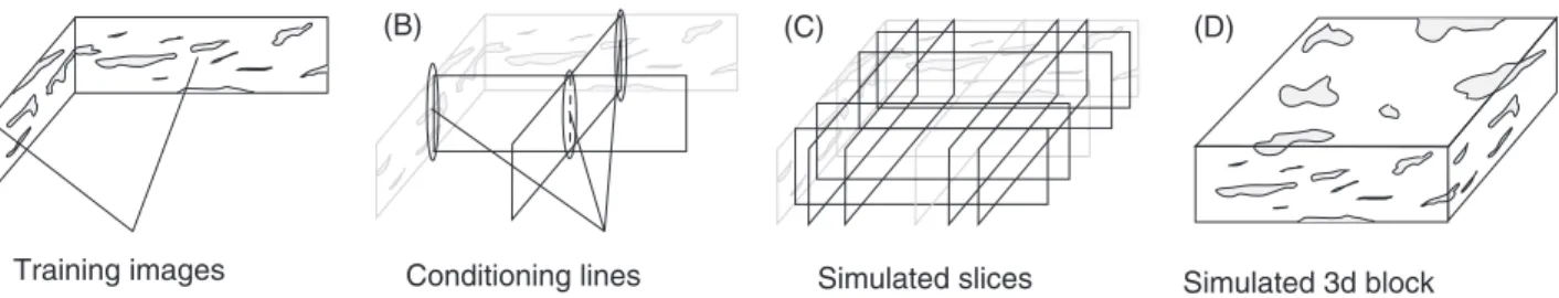
The 3D simulations were performed at the scale of the mapped block shown in Figure 5. The block includes 72 million nodes (600× 600 × 200) and is discretized at 1-cm resolution. In this way, the block can be fully conditioned on the outer sides with four mapped sections. For both algorithms (TP and MPS), 10 realizations were computed for the unconditional and the conditional case. The MPS simulations were performed using a technique that is described by Comunian et al. (2011a) and that allows to overcome the lack of a 3D TI. The 3D domain is filled with 2D simulations along a sequence of 2D slices in both directions. The data simulated in the previous slices as well as the TIs at the boundary of the domain are used to condition the following 2D simulations (Figure 4). This sequential simulation procedure was repeated until the 3D block was completed. Instead of using a single cross section as TI, we constructed a larger TI with all four cross sections combined in a horizontal series. This measure may improve the simulation of nonstationary characteristics, for example, varying sizes of geobodies, by creating repetitive patterns on the TI itself.
(A) (B) (C) (D)
Training images Conditioning lines Simulated slices Simulated 3d block
Figure 4. Illustration of sequential simulation approach to model a 3D domain with MPS based on 2D TIs (Comunian et al. 2011a). The block is simulated in slices, which are conditioned to each other and stepwise fill the model domain slice by slice. The pictures show two perpendicular training images (A), the first conditioned simulations (B), an ensemble of simulated slices (C) and finally the complete 3D simulation (D).
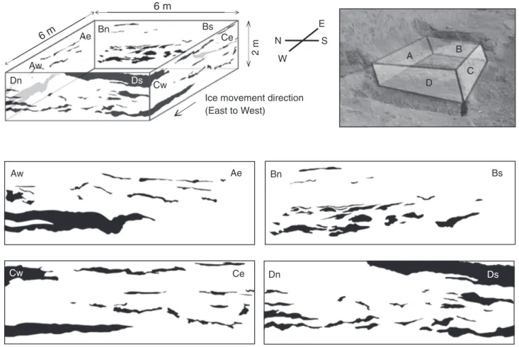
Dn 6 m 2 m 6 m E S N W
Ice movement direction (East to West) A D C B Aw Ae Bn Bs Cw Ds Bn Ae Ce Dn Ce Ds Bs Aw Cw
Figure 5. Mapped till cross sections with sand lenses. The upper pictures show the orientations and dimensions of the excavated block of clayey till. Section A is hereby part of the profile face. Sections A and C are recorded longitudinal to the ice movement direction, whereas B and D show outcrops perpendicular to the deformation direction. All sections are 6-m long and 2-m high. The cross sections are illustrated in detail below, where the black geobodies indicate sand lenses and the white background category represents the clayey matrix.
Results
Mapping Till Cross Sections
Figure 5 shows the excavated block and the associ-ated cross sections that were mapped in the field. Sections A and C are oriented parallel to the ice-movement direction and Sections B and D perpendicularly. Visual inspection of mapped geobodies on the four cross sections (lower graphs on Figure 5) yield differences regarding size, variability, and distribution. The term geobody char-acterizes architectural elements (Labourdette and Jones 2007) and is used here as a term for an embedded geolog-ical feature below the stratigraphic level. In the parallel sections A and C most geobodies are elongated sand stringers in nearly horizontal position. They seem ran-domly distributed with no apparent spatial trend. A large sand body near the lower edge of Section A outranges the scale of the sand stringers by several orders. A similar sand body is observed at the top edge of Section D mark-ing a transition from where no more sand strmark-ingers occur. The horizontal extent of such features reaches several meters and is only partly displayed on the sections. The remaining geobodies in Section D have more complex shapes indicating nonstationary deformation in multiple
directions as explained by Kessler et al. (2012). Similarly, the geobodies in Section B range between stringers and pockets and seem to be aligned along a tilted plane stretch-ing from the lower left to the upper right of the section. Most features are visibly shorter and less anisotropic com-pared to their equivalents on Section D and concentrate in the lower half of the section. The close positioning to each other further evidences a spatial trend in verti-cal direction. This section has 38 features with the largest number of sand lenses (Table 2). In comparison with the other sections the size of the features is rather uniform with no exceptionally sized lenses being present.
Geometry of Sand Lenses
The geometry of geobodies was described with their size, length in horizontal direction, thickness, anisotropy ratio, and shape factor (Table 2). The shape factor is a scalar and describes the proportion of the observed geo-body compared to an elliptic geogeo-body defined by the long and the short axes of the same feature. It is cal-culated as the ratio between the true area and the area of the convex shape. Table 2 supports the visual inspec-tion showing that the geometry of lenses on Secinspec-tion B differs significantly. On Sections A, C, and D the mean
of lengths and thicknesses range between 50 and 75 cm and 10 and 15 cm, respectively. The corresponding mean length for Section B is significantly smaller at 35 cm. The average size of B is also smallest with less than a third of the mean size of the other sections. The vertical anisotropy is fairly constant at ratios between 4.0 and 5.6. Surprisingly, a comparison between the Sections A and C (parallel to ice movement) and B and D (perpendicular) does not yield measurable horizontal anisotropy (lx/ly). Glaciers move locally in different directions depending on the topography of the bed and shear deformation is not necessarily uniformly oriented along the overall ice movement at local scale. Considering the multidirectional deformation of glacial sediments, the missing horizontal anisotropy may not be true for sand lenses at different till locations.
Spatial Variability of Sand Lenses
With regard to the identification of nonstationary pat-terns of geobodies in a 2D domain, the measures of spatial correlation are of great importance. Correlation of cat-egorical data is commonly studied with variogram or covariance-based indicator geostatistics (Ritzi 2000; He et al. 2009). The experimental (indicator-) variograms for all four sections were computed in horizontal and verti-cal direction (Figure 6) using the minimum distance or lag of 1 cm between two data points. Due to the variable size and geometry of sand lenses on each section it is not straight forward to find a mathematical function to fit the experimental variogram. For Sections A, C, and D nested structures using both exponential and Gaussian models were used to find the best fit.
The range in horizontal direction is comparable for Sections A, C, and D. The first structure shows a correlation length between 90 and 130 cm and the second structure between 280 and 400 cm, respectively. The horizontal correlation for Section B is significantly smaller and can be approximated with only one structure at a length of 130 cm. Ranges in vertical direction vary between 20 and 55 cm evidencing vertical anisotropy of single sand lenses. Since the sill is about equal for both horizontal and vertical direction, we assume geometric but no zonal anisotropy within the sections. Interestingly, there is a decline of the variance in vertical direction at large lags. The sand lenses in Sections A through C do not cut the edges of the image meaning that there is strong correlation at the maximum lag of 200 cm. Since sand lenses have thin shapes and horizontal orientation, periodic signals are expected for layered lithological or sedimentary structures. Periodicity occurs if repetitive patterns, in this case, recurrent sand lenses are present in the data. It is also indicated in the experimental variograms with fluctuations around the sill. A similar effect of inconsistencies near the maximum lag is visible for Section B in horizontal direction. However, a good variogram fit at multiple lag distances beyond the correlation lengths is less important. An inconvenient property of Sections C and D is the unbound pattern of the data toward larger lags. The missing sill at large lags
Table 1
Ratios of Simulated Pixels with Sand Facies
Reference Image No. of Vertical Data Columns MPS (%) TP (%) C 3 43.5 31.9 7 60.8 32.9 D 3 12.9 14.1 7 58.1 27.2
The percentage indicates how many pixels with sand facies on the reference image were reproduced on the simulations. The ratios are given for both reference images and for both conditioning scenarios with three and seven data columns, respectively.
is due to nonstationary behavior of the data, particularly because of a spatial trend. The size of the geobodies in these sections varies and declines from the left toward the right edge of the section.
Simulation of Parallel Sections
Visual Inspection
Figure 7 shows the training and reference image and one realization of each of the simulation ensembles for the scenario C-A (simulating Section C from A). Visual inspection of the unconditional simulations evidences dif-ferences between the TP and MPS method. The simulated lenses with the TP method are more uniform in terms of size and anisotropy. This is due to the fact that mean lengths are used for simulation and thus the deviation from the average geometry is small. The MPS method has a larger spread simulating elongated sand lenses beyond and below the correlation lengths. The difference is more evident comparing the conditioned realizations. The MPS method has less artifacts and accounts better for connected features between conditioning points at 1 m distance. The realizations of the second scenario D-B simulating section image D from B are less satisfying. The corre-lation lengths of the lenses in Section B are only half the size compared to the reference Section D. Both meth-ods, and in particular the TP approach, have difficulties in reproducing the elongated and rather large structures in Section D.
Both methods cannot reproduce adequately the vari-ability in size and the spatial trends observed in Sections A and B. Difficulties with simulating nonstationary patterns are expected particularly for the unconditioned case. The sand lenses are random distributed and there is no signif-icant advantage of either method. Nonstationary patterns, particularly regarding varying size, are better reproduced using conditioning data, but only using 1-m spaced data columns yield a visible improvement.
The impact of the conditioning data was evalu-ated calculating the probability maps of the realiza-tions reproducing each pixel on the reference section. The 50%-quantile of sand pixels simulated on all real-izations was selected as the simulated average. This
Cross section A Horizontal 0.20 0.15 Variance γ(h) 0.0 Vertical 0.05 0.10 0 200 Lag distance h [cm] Variance γ(h) 120 80 40 160 o o o o o o o o o o o o o o o o o o o o o o o o o o o o o o o o o o o o o o o o o o o o o o o Cross section B o o o o o o o o o o o o o oo o o o o o o o o o o o o o o o o o o o o o o o o o o o o o o o o o Cross section C o o o o o o o o o o o o oo o o o o o o o o o o o o o o o o o o o oo o o o o o o o o o o o o o o o Cross section D o o o o o o o o o o o o o o o o o o o o o o o o o o o o o o o o o o o o o o o o o o o o 0.20 0.15 0.0 0.05 0.10 0.20 0.15 0.05 0.10 o 0.20 0.15 0.0 0.05 0.10 o 0.20 0.15 0.0 0.05 0.10 o 0.20 0.15 0.0 0.05 0.10 0.20 0.15 0.0 0.05 0.10 0.20 0.15 0.0 0.05 0.10 0 200 400 600 Lag distance h [cm] 0 200 400 600 Lag distance h [cm] 0 200 400 600 Lag distance h [cm] 0 200 400 600 Lag distance h [cm] 0 200 Lag distance h [cm] 120 80 40 160 0 200 Lag distance h [cm] 120 80 40 160 0 200 Lag distance h [cm] 120 80 40 160
Figure 6. Experimental variograms for all four Sections A to D including modeled variogram using a simple (Section B) or a nested model (Sections A, C, and D). The upper four diagrams are in horizontal direction. The lower four diagrams are in downward direction. 0 100 200 300 400 500 600 0 100 200 300 400 500 600 0 100 200 300 400 500 600 0 100 200 300 400 500 600 0 100 200 300 400 500 600 0 100 200 300 400 500 600 200 100 0 200 100 0 200 100 0 Training image, section A
TP conditioned with 7 columns, simulation TP unconditioned, simulation 200 100 0 200 100 0
MPS unconditioned, simulation MPS conditioned with 7 columns, simulation 200
100
0
Reference image, section C
Figure 7. Cross sections and realizations. The left column shows the TI (Section A) and the unconditional simulations with transition probability and multiple-point simulation. The right column shows the reference image (Section C) and the realizations with seven conditioning data columns.
probability map was compared to the actual reference image C. The percentages of coinciding sand pixels on both images were calculated and are tabulated in Table 1.
The probability of reproduced sand pixels is a good indicator for the quality of simulations. For the case with seven conditioning data columns, the ratios are comparable for both reference Sections C and D. The MPS method reaches ratios twice as high compared to the TP method indicating much better reproduction of the reference image. It is due to the fact, that the MPS method simulates more anisotropic geobodies and therefore captures the sand facies in between two
conditioning lines. This highlights the advantages of MPS when simulating rich datasets. The ratio of nearly 60% for both cases is promising with regard to the nonstationarity of the cross sections. The performance declines if only three columns are used. Especially for Section D, the facies ratio is rather poor with only 13% to 14%. The sand lenses on training Section B are smaller compared to the spacing of the columns and only a few pixels in the vicinity of the conditioning columns are reproduced. In practice, conditioning datasets at 1 m or even 2 m spacing are rarely available and the rapid decline of the number of simulated sand pixels show the dependence on conditioning data to reproduce the reality.
Statistical Analysis of Simulated Features
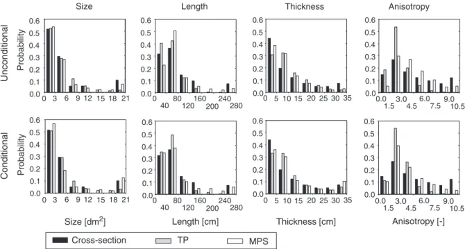
A geometric evaluation of simulated geobodies was done calculating the statistics on the ensemble of realizations. Mean and maximum values are summarized in Table 2 and histograms of the distribution of geometric parameters are provided in Figure 8. The analysis passes on the consideration of the conditional scenario with only three columns, since the effect on the geometric prop-erties compared to the unconditioned case is minor. To evaluate the quality of simulated geobodies relative to the mapped geobodies, the parameters size, length, thickness, anisotropy, and shape factor were considered. In addition, the number of simulated geobodies was compared for the reference and the simulated cross sections.
Despite the fixed facies proportions for the simula-tions, there are substantial differences in the number of simulated geobodies. The MPS method is closest to reality with an average of 37 simulated lenses compared to 20 on reference image C for the unconditional case. The numbers for Section D are 28 and 26, respectively. Con-ditioning yields an almost perfect match at 19 and 27 for Sections C and D. The TP method simulates about twice the number of geobodies compared to the reference image, with a mean of 54 geobodies for Section C and 71 for Section D. Conditioning produces only minor improve-ment. The comparison of the individual geometric param-eters is reported in Table 2.
The histograms are only shown for Section C as the distribution for Section D does not yield large differences. The reference scenario for the histograms is based on the mapped sand lenses observed on Section C. The inter-vals for the histogram were defined using seven bins and capturing at least 95% of all geobodies. The size distribu-tion is well reproduced for the abundant smaller features but denotes some deficiencies for larger-sized features particularly for the TP method. The MPS method bet-ter reproduces the mean size of the mapped lenses of 7.65 dm2, particularly in the conditioned case. Similar is true for the parameter length. TP indicates smaller hori-zontal extents with a mean value of 35.7 cm compared to 74.0 cm for the reference image and 56.8 cm for the MPS method. The difference in producing features beyond the correlation length is also obvious looking at the maximum values. TP underestimates more than MPS the maximum extent of sand lenses with only 142 cm. The longest fea-tures on the MPS simulation are located around 300 cm, which is much closer to the reality on the reference image at 304 cm. The conditioning yields particular improve-ment for the MPS simulations. While the mean length remains the same, the length distribution is closer to the one of the reference images. The anisotropy clarifies the significant differences between the TP and MPS method. Mean anisotropy ratios are found for the reference images at 5.6, for the MPS at 4.6 and for the TP at 2.7. The MPS method simulates elongated sand lenses in the full range from ratios of 2 to 10, whereas the TP method is limited to anisotropic shapes at ratios from 1 to 4.
The histograms for Section D show similar tenden-cies. Mean lengths and anisotropy are generally smaller,
due to the exceptional training patterns on Section B. The differences between TP and MPS are even more pro-nounced because the even smaller mean lengths and a large proportion at 19% for Section D. These factors result in a larger number of features (71) for the TP method. On the other hand, the positive conditioning effect is clearer for the B to D simulation. The MPS method par-ticularly benefits and reproduces better mean lengths and thicknesses.
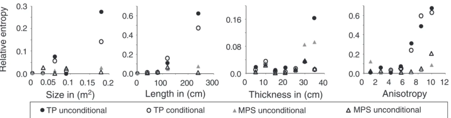
We compare the geometric parameters from the ref-erence image (Section C) and the corresponding sim-ulations in terms of the relative entropy (Figure 9). The relative entropy is a measure of the difference between two probability distributions of the same param-eter (Kullback 1968). The graphs emphasize the poor performance of the TP method at extreme geometries. Size, length, and anisotropy are all inadequately repro-duced for large values. The entropy also shows that con-ditioning effect on the geometry of geobodies has minor effect at smaller distances. Only sand lenses thicker 25 cm and strongly anisotropic shapes seem to benefit from the conditioning.
The analysis of the geometry of sand lenses for the two simulation algorithms evidence good capabilities to reproduce the geometry and anisotropy of small geobodies below the correlation lengths. MPS has advantages regarding larger geobodies and conditioning supports the simulation of extreme geometries. Since larger geobodies are believed to be especially important for the hydraulic conditions, MPS seems to be the more appropriate method for the simulation of sand lens geometries.
Connectivity and Equivalent Permeability
Connectivity functions for sand lenses can be defined such as the probability that two points separated by a distance h along a given direction belong to the same geobody (for a rigorous definition of connectivity functions, see Allard [1992] and Renard and Allard [2012]). The graphs in Figure 10 show the connectivity functions for cross section C using the average of an ensemble of 100 realizations simulated with TP and MPS. The reference image and the simulations both have sand facies proportions of 13% and no connectivity in either direction is achieved at full extent of the 2D scenario. For the unconditional case, the connectivity on the reference image is in both directions greater than for the simulations at all lags. Along the horizontal direction, the x-axis is met at a lag of 300 cm, which corresponds to the horizontal extent of the single-large feature in the lower half of the reference image (Figure 5). The MPS function is closer to the reference image curve reaching the point of no connectivity at a similar lag distance. The TP curve has a much steeper decline and relevant connectivity is lost at a range of less than 100 cm. In downward direction the connectivity functions for the two methods are comparable.
Conditional simulations do not yield much improve-ment in terms of connectivity. The MPS function almost reproduces the TI curve especially in the downward
Table 2
Statistics on the Geometry of Mapped and Simulated Sand Lenses
Size [dm2] Length [cm] Thickness [cm] Anisotropy [lh/lv] Section (No of Columns) No. of Lenses Proportion
[Sand] Mean Max Mean Max Mean Max Mean Max
Shape Factor Reference A 21 12.3% 7.00 118.9 52.0 363 12.0 58.4 4.3 15.3 0.251 B 38 7.0% 2.20 11.5 35.0 116 9.0 33.9 4.0 10.7 0.141 C 20 12.8% 7.65 68.7 74.0 314 14.0 52.4 5.6 14.3 0.158 D 26 19.1% 8.80 118.9 66.0 353 15.0 62.6 4.0 12.4 0.238 TP C (0) 54 12.8% 2.88 18.6 35.7 142 12.7 40.3 2.7 6.8 0.145 C (7) 44 13.2% 3.62 24.0 41.2 149 13.6 54.8 3.1 5.9 0.148 D (0) 71 18.4% 3.14 20.6 37.6 144 13.1 45.7 3.0 7.2 0.192 D (7) 62 18.5% 3.61 29.7 39.0 154 14.0 61.6 3.1 7.2 0.193 MPS C (0) 37 12.4% 4.08 39.6 56.8 299 11.6 41.5 4.6 11.7 0.136 C (7) 19 12.4% 8.05 57.3 68.9 299 15.1 50.4 4.1 10.2 0.147 D (0) 28 18.4% 8.22 41.7 90.8 310 16.0 48.9 5.8 11.2 0.202 D (7) 27 19.8% 9.04 87.0 74.0 333 17.1 68.7 4.9 10.0 0.220
Statistics on the geometry of mapped and simulated sand lenses. Mean and maximum values are calculated for the geometric parameters size, length, thickness, and anisotropy. In addition, the shape factors are given for the ensemble of geobodies. The calculations were done for all four cross sections and for both algorithms (TP and MPS) including the unconditioned (0 data columns) and conditioned (7 data columns, 1 m distance) case.
direction, whereas the TP function remains unchanged. The results for the second scenario simulating Section D from B resemble the first scenario and show the same patterns described above. The graphs show that the con-nectivity is controlled by the size of the largest observed or simulated geobodies and not by the frequency or configuration in space. This finding is in accordance with
the visual inspection of the mapped cross sections and was expected for sand proportions of 20% and less (Stauf-fer and Aharony 1994; Hunt and Ewing 2009). However, the connectivity of the MPS simulation is rather close to the one of the reference image in horizontal direction and show promise to be able to reproduce the horizontal transport behavior with such an approach.
0.0 0.1 0.2 0.3 0.4 0.5 0.6 21 6 9 18 3 0 Unconditional Conditional 15 12 Size [dm2] 280 80 120 240 40 0 200 160 Length [cm] 35 10 15 30 5 0 20 25 10.5 3.0 4.5 9.0 1.5 0.0 7.5 6.0 Thickness [cm] Anisotropy [-]
Size Length Thickness Anisotropy
Probability 0.0 0.1 0.2 0.3 0.4 0.5 0.6 0.0 0.1 0.2 0.3 0.4 0.5 0.6 0.0 0.1 0.2 0.3 0.4 0.5 0.6 0.0 0.1 0.2 0.3 0.4 0.5 0.6 0.0 0.1 0.2 0.3 0.4 0.5 0.6 0.0 0.1 0.2 0.3 0.4 0.5 0.6 0.0 0.1 0.2 0.3 0.4 0.5 0.6 21 6 9 18 3 0 12 15 280 80 120 240 40 0 200 160 0 5 10 15 20 2530 35 10.5 3.0 4.5 9.0 1.5 0.0 7.5 6.0 Probability Cross-section TP MPS
Figure 8. Histograms of the parameters size, length, thickness, and anisotropy of the simulations aimed at reproducing the reference cross section C. The upper histograms show the statistics for the unconditional simulations and the lower row for the conditional simulations with seven vertical data columns.
20 30 40 0.0 0.1 0.2 0.3 0 0.05 0.1 0.0 0.2 0.4 0.6 0 100 200 300 0.0 0.08 0.16 0 0.15 0.2 10 0.0 0.2 0.4 0.6 0 2 4 6 8 10 12 Relative entropy
Size in (m2) Length in (cm) Thickness in (cm) Anisotropy
TP unconditional TP conditional MPS unconditional MPS unconditional
Figure 9. The relative entropy for the geometric parameters size, length, thickness, and anisotropy. The four data series represent the divergence between the reference image and the different simulations (TP and MPS for both the conditional and unconditional case). Please note the different scaling of the entropy for the different parameters.
0 100 200 300 400 0.0 0.2 0.4 0.6 0.8 1.0 Horizontal direction Lag [cm] tau ( h ) 0 20 40 60 80 100 Lag [cm] Downward direction Section TP MPS 0 100 200 300 400 0.2 0.4 0.6 0.8 1.0 Lag [cm] tau ( h ) 0.0 0.0 0.2 0.4 0.6 0.8 1.0 tau ( h ) 0 20 40 60 80 100 Lag [cm] 0.0 0.2 0.4 0.6 0.8 1.0 tau ( h )
Section C - Unconditional Section C - Conditional
Horizontal direction Downward direction
Section TP MPS Section TP MPS Section TP MPS
Figure 10. Connectivity functions tau(h) describing the probability that two points on a realization being connected by continuous paths through the same lithofacies.
Another criterion to compare the simulation and the reference image is to compute the equivalent hydraulic conductivity tensors Keq of both images. For that purpose, a constant hydraulic conductivity value has been associated to each facies (5.0× 10⁻⁸m/s for the clayey matrix and 5.0× 10⁻⁴ m/s for the sand lenses). For each configuration, two flow simulations are performed with prescribed heads linearly varying along the boundary of the domain (Long et al. 1982). The equivalent conductivity tensor is then computed from the results of these two flow simulations (see, e.g., Renard and de Marsily 1997). To compare the results with its reference, we compute a relative error by using the Frobenius norm of a tensor, which is defined as the square root of the sum of the absolute squares of its elements (Weisstein 2012). In particular, the Frobenius norm of the difference between the computed and reference tensors, divided by the Frobenius norm of the reference tensor is considered. In Figure 11, this relative error is displayed for the reference section C.
The relative errors are small and fairly similar for the different simulations because connected paths cutting both edges of the image are neither present on the reference
0.0 0.5 1.0 1.5 2.0 2.5 3.0 3.5 MPS cond. (3 col)
Relative error on frobenius norms
MPS cond. (7 col) MPS uncond TP cond. (7 col) TP cond. (3 col) TP uncond 4.0
Figure 11. Box plot of the Frobenius norm errors of the
K equivalent tensors. The graphs indicate the error of
the K equivalent between the reference image C and the simulations for the same section. The errors are shown for both algorithms (TP and MPS) and for the unconditioned and conditioned cases (with 3 and 7 data columns).
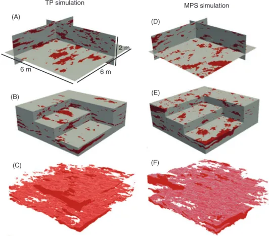
(A) (B) (C) (D) (E) (F) TP simulation MPS simulation 6 m 2 m 6 m
Figure 12. Three-dimensional realizations of simulated sand lenses in till blocks. The pictures (A) to (C) show one realization of an ensemble of 10 simulations performed with TP and pictures (D) to (F) an equivalent realization done with MPS. The simulations are conditioned with four TIs fencing the simulated block. Images (A) and (D) show fence diagrams, (B) and (E) complete simulated blocks and (C) and (F) show only the sand lenses without the till matrix.
0 100 200 300 400 0.0 0.2 0.4 0.6 0.8 1.0 Horizontal direction Lag [cm] tau ( h ) 0 50 100 150 200 Lag [cm] Vertical direction TP MPS 0.0 0.2 0.4 0.6 0.8 1.0 tau ( h ) TP MPS
Figure 13. Connectivity functions for 3D simulations. The graphs illustrate the connectivity of one realization of either method (TP and MPS) and in both, horizontal and vertical direction.
image nor on the simulations. The spread of the MPS simulations evidences the largest variability of simulated geobodies and demonstrates that MPS generates a broader range of geometries. It also shows that the location of the individual lenses is important for the connected pathways, as the unconditional simulations have the largest error. The higher conditioned the simulations, are the more become the positions of lenses controlled and resemble
the reference image. The simulations tend to converge to a much narrower space. The TP simulations have in contrast a small variability of geometries and therefore a minimal spread for all scenarios. The probability to form conductive paths is much reduced, due to the simulation of smaller lenses. The Eigen values of the K tensor show that the flow direction is the same for both the reference image and the two simulation techniques. The main component of the hydraulic flow vector is sub-horizontal, in line with the orientation of the main axis of the sand lenses.
Simulation of a 3D Block
It is well-known that the critical proportions of facies that create connected flowpaths vary significantly with the number of dimensions (e.g., Hunt and Ewing, 2009). The aim of the 3D simulation is to investigate a potentially different connectivity pattern in three dimensions rather than the reproduction of a specific section image. A second analysis of the geobodies and their distribution in 3D is not reported here, because the applied simulation algorithms and the measures of correlation (TP) and the type of TI remained the same from the 2D simulations. The domain is only conditioned on the outer boundaries and no additional vertical data columns were used for conditioning the interior of the block. The interior of the
realization is thus expected similar to the unconditioned case in 2D. This assumption was approved by visual inspection of the individual sections of the block. One example of the 3D ensemble of conditioned realizations is presented in Figure 12 for both simulation algorithms (TP and MPS).
The connectivity in three dimension marks an impor-tant parameter to highlight the difference between mul-tidimensional simulations. The connectivity functions in Figure 13 show the unconditional case for the TP and MPS method. Despite the steep decline, both functions level off at around 0.1 for the MPS and 0.03 for the TP realization. This means that connectivity of the sand facies is conceivable within the entire block. Interestingly, the TP method has a smoother decline in vertical direction, due to the influence of the thick feature in the parameter-ized section A. In contrary, the MPS simulation uses an anisotropic search template avoiding unrealistically thick geobodies in favor of elongated shapes. The TP graph shows a small increase toward the maximum lag. This behavior is typical for curvilinear and complex structures. Overall, the level of connectivity at large distances is low but consistently higher than zero for both models.
Discussion
Outcrop studies of glacial tills at the decimeter to meter scale are important to get some quantitative char-acterization of the fine-scale heterogeneity of sand lenses including their size, shape, frequency, and spacing. Field measurements are challenged with different types of sand lenses occurring at varying scales and dimension. Map-ping of large sand layers demands extended cross sections, which hinder a fine spatial resolution. A discretization of maximum few centimeters is recommended to cap-ture the facies struccap-tures and thin connectivity between sand stringers. Sand lenses have characteristic, elongated shapes with strong anisotropy in x- and z-direction. The anisotropy can be sufficiently described with simple geo-metric parameters, such as length and thickness, and are supported by shape factor calculations. Critical nonsta-tionary patterns on cross sections are minor spatial trends in vertical direction and large variation in terms of the size of individual geobodies. The variable size complicates the calculation of statistical moments for a limited sample of measured sand lenses.
To model this type of heterogeneity, the TP algo-rithm is interesting, because parameterization is limited to transiograms, which are related to the mean lengths and facies proportions that are easy to infer from dig-ital section images. However, here we show that TP lacks the ability to simulate the wide range of geome-tries that are present in the mapped sections. The MPS method has more advanced capabilities reproducing com-plex geometries of sand lenses, because it is based on a more sophisticated (multiple-point) statistical model. Dense conditioning enables a rather exact reproduction of a targeted section image. The spacing should not be much larger than the correlation length of sand lenses, since
a distance of 2 m between data columns already caused a significant decline in performance. Borehole logs at 2 m spacing and below are in most practical applications unfeasible and the presented conditioning scenarios are theoretical. However, if correlation lengths of sand lenses increase the efficacy of conditioning scenarios become of more practical value. An important limitation of both methods is the consideration of spatial trends on the cross section. The TP method has the advantage to easy upscale simulations to three dimensions, because spatial correla-tion is described with one-direccorrela-tional Markov models in each principal direction separately. MPS models need to simulate 3D domains with a more complicated sequential simulation of 2D slices.
The connectivity of sand lenses depends on the geom-etry of the individual geobodies and on the numbers and distribution in space. At sand facies proportions of less than 20% the maximum connectivity in 2D is equal to the maximum extent of individual sand lenses. It is thus crucial to choose appropriate scales for the cross sections to ensure the inclusion of larger sand bodies and sand sheets. The simulations obtained in three dimensions show enhanced connectivity compared to the 2D simulations. Of course, those results are based only on the available 2D data and on the stochastic models. The existence of connections cannot be proved with the applied data and methods. Nonetheless, we are quite confident that those results are reasonable for three reasons: first, the results are obtained with two different methods that are based on different random field models; secondly, these two methods have proved to give reasonable results in 2D when they could be tested against field observations; and, thirdly, it is well known in percolation theory that con-nectivity patterns may be very different in 2D and 3D. For all those reasons, we think that our results provide a clear indication that such large-scale connectivity may indeed exist. If this is true, it may have important implica-tions on the large-scale hydrogeological behavior of such systems. This implies that additional research should be conducted to reject or confirm our results using further field experiments.
In addition, the connectivity of sand lenses may be further enhanced by secondary flowpaths, for example, vertically oriented fractures. Conjugated tectonic fractures have been observed at numerous till sites (Klint and Gravesen 1999; Klint 2001) and were included in transport models for tills, for example, as secondary porosity (Jørgensen et al. 2002, 2004; Chambon et al. 2010). These may facilitate transport of, for example, contaminants toward or through sand lens horizons and thus increase the connectivity between sand lenses. With regard to high hydraulic conductivities of sand lenses compared to the low-permeability till matrix connected channel networks comprising fractures and sand lenses may be crucial for horizontal transport as pointed out by Fogg et al. (2000). It is particularly relevant for the transport of contaminants, even if the channels occur at the thickness of thin sand stringers (mm to cm). The fine scale characterization of heterogeneity in tills is therefore needed to assess the
transport regime of water and contaminants in clayey tills.
Conclusions
The study reveals that sand lenses occurring in tills represent a complex type of heterogeneity in terms of scale, shape, and geometry. The inclusion of fine-scale heterogeneity is crucial to improve solute transport mod-els for aquitards in glacial settings. MPS have shown better capabilities to simulate the anisotropic shapes of sand lenses compared to TP-based approaches. The repro-duction of complex structures is particularly important to evaluate connectivity between features in three dimen-sions. The sequential simulation approach to achieve 3D realizations from 2D outcrop data with the MPS method was found appropriate to overcome the lack of 3D TIs. The 3D simulations suggest narrow connection between individual sand lenses that may affect the hydraulic conductivity of till settings. However, a final proof of connectivity to verify the simulations can only be done with 3D field excavations for such type of heterogeneity.
Acknowledgments
This study was conducted as part of a project to characterize the hydrogeology of contaminated sites in Denmark and was supported by the Technical Univer-sity of Denmark, the Geological Survey of Denmark and Greenland (GEUS) and REMTEC, Innovative REMedia-tion and assessment TEChnologies for contaminated soil and groundwater, Danish Council for Strategic Research. We would like to thank the Kallerup gravel pit for pro-viding access to the study site and great support during the excavations.
References
Allard, D. 1992. On the Connectivity of Two Random Set Models: The Truncated Gaussian and the Boolean. Dordrecht, The Netherlands: Kluwer Academic Publications.
Arpat, G., and J. Caers. 2007. Conditional simulation with patterns. Mathematical Geology 39: 177–203.
Asprion, U., and T. Aigner. 1997. Aquifer architecture analysis using ground-penetrating radar: Triassic and Quaternary examples (Southern Germany). Environmental Geology 31: 66–75.
Bastante, F.G., C. Ordonez, J. Taboada, and J.M. Matias. 2008. Comparison of indicator kriging, conditional indicator simulation and multiple-point statistics used to model slate deposits. Engineering Geology 98: 50–59.
Bayer, P., P. Huggenberger, P. Renard, and A. Comunian. 2011. Three-dimensional high resolution fluvio-glacial aquifer analog: Part 1: Field study. Journal of Hydrology 405: 1–9. Bertran, P., and J.-P. Texier. 1999. Facies and microfacies of
slope deposits. Catena 35: 99–121.
Broholm, K., B. Nilsson, R.C. Sidle, and E. Arvin. 2000. Transport and biodegradation of creosote compounds in clayey till, a field experiment. Journal of Contaminant Hydrology 41: 239–260.
Carle, S.F. 1996. A transition probability-based approach to geostatistical characterization of hydrostratigraphic archi-tecture. Ph.D. thesis, University of California, USA.
Carle, S.F. 1999. T-PROGS: Transition Probability Geostatisti-cal Software. Users Manual. USA: University of California. Carle, S.F., and G.E. Fogg. 1996. Transition probability-based indicator geostatistics. Mathematical Geology 28: 453–476.
Carle, S.F., E.M. LaBolle, G.S. Weissmann, D. van Brocklin, and G.E. Fogg. 1998. Conditional simulation of hydrofacies architecture: A transition probability/Markov approach. In Hydrogeological Models of Sedimentary Aquifers, ed. G.S. Fraser and J.M. Davis. Society for Sedimentary Geology. Special Publication: 147–170.
Chambon, J.C., M.M. Broholm, P.J. Binning, and P.L. Bjerg. 2010. Modeling multi-component transport and enhanced anaerobic dechlorination processes in a single fracture-lay matrix system. Journal of Contaminant Hydrology 112: 77–90.
Comunian, A., P. Renard, and J. Straubhaar. 2011a. 3D multiple-point statistics simulation using 2D training images. Com-puters & Geosciences 40: 49–65.
Comunian, A., P. Renard, J. Straubhaar, and P. Bayer. 2011b. Three-dimensional high resolution fluvio-glacial aquifer analog: Part 2: Geostatistical modeling. Journal of Hydrol-ogy 405: 10–23.
Cuthbert, M.O., R. Mackay, J.H. Tellam, and R.D. Barker. 2009. The use of electrical resistivity tomography in deriving local-scale models of recharge through superficial deposits. Quarterly Journal of Engineering Geology and Hydrogeology 42, no. 2: 199–209.
dell’Arciprete, D., R. Bersezio, F. Felletti, M. Giudici, A. Comunian, and P. Renard. 2012. Comparison of three geostatistical methods for hydrofacies simulation: A test on alluvial sediments. Hydrogeology Journal 20: 299–311. Deutsch, C.V., and A.G. Journel. 1992. GSLIB: Geostatistical Software Library and User’s Guide. New York: Oxford University Press.
Dreimanis, A. 1993. Small to medium-sized glacitectonic structures in till and in its substratum and their comparison with mass movement structures. Quaternary International 18: 69–79.
Eaton, T.T. 2006. On the importance of geological heterogeneity for flow simulation. Sedimentary Geology 184: 187–201. Eyles, N. 2006. The role of meltwater in glacial processes.
Sedimentary Geology. 190: 257–268.
Falivene, O., P. Arbu´es, A. Gardiner, G. Pickup, J.A. Mu˜noz, and L. Cabrera. 2006. Best practice stochastic facies modeling from a channel-fill turbidite sandstone analog (the Quarry outcrop, Eocene Ainsa basin, northeast Spain). AAPG Bulletin 90, no. 7: 1003–1029.
Feyen, L., and J. Caers. 2006. Quantifying geological uncer-tainty for flow and transport modeling in multi-modal het-erogeneous formations. Advances in Water Resources 29, no. 6: 912–929.
Fogg, G.E., S.F. Carle, and C. Green. 2000. Connected-Network Paradigm for the Alluvial Aquifer System. USA: Geological Society of America.
Fogg, G.E., C.D. Noyes, and S.F. Carle. 1998. Geologically based model of heterogeneous hydraulic conductivity in an alluvial setting. Hydrogeology Journal 6: 131–143. Fraser, G.S., and J.S. Cobb. 1982. Late Wisconsinan proglacial
sedimentation along the West Chicago Moraine in north-eastern Illinois. Journal of Sedimentary Research 52, no. 2: 473–491.
Gerber, R., J. Boyce, and K. Howard. 2001. Evaluation of heterogeneity and field-scale groundwater flow regime in a leaky till aquitard. Hydrogeology Journal 9: 60–78. Goovaerts, P. 1999. Geostatistics in soil science: State-of-the-art
and perspectives. Geoderma 89: 1–45.
Harrar, W., L. Murdoch, B. Nilsson, and K.E. Klint. 2007. Field characterization of vertical bromide transport in a fractured glacial till. Hydrogeology Journal 15: 1473–1488.
Harrington, G.A., M.J. Hendry, and N.I. Robinson. 2007. Impact of permeable conduits on solute transport in aquitards: Mathematical models and their application. Water Resources Research 43, no. 5: W05441.
He, Y., K. Hu, B. Li, D. Chen, H.C. Suter, and Y. Huang. 2009. Comparison of sequential indicator simulation and transition probability indicator simulation used to model clay content in microscale surface soil. Soil Science 174, no. 7: 395–402.
Hendry, M.J., C.J. Kelln, L.I. Wassenaar, and J. Shaw. 2004. Characterizing the hydrogeology of a complex clay-rich aquitard system using detailed vertical profiles of the stable isotopes of water. Journal of Hydrology 293: 47–56. Houmark-Nielsen, M. 2007. Extent and age of Middle and Late
Pleistocene glaciations and periglacial episodes in southern Jylland, Denmark. Bulletin of the Geological Society of Denmark 55, no. 1: 9–35.
Houmark-Nielsen, M. 2003. Signature and timing of the Kattegat Ice stream: Onset of the last glacial maximum sequence at the southwestern margin of the Scandinavian Ice Sheet. Boreas 32, no. 1: 227–241.
Hu, L.Y., and T. Chugunova. 2008. Multiple-point geostatistics for modeling subsurface heterogeneity: A comprehensive review. Water Resources Research. 44, no. 11: W11413. Huggenberger, P., E. Meier, and A. Pugin. 1994.
Ground-probing radar as a tool for heterogeneity estimation in gravel deposits: Advances in data—Processing and facies analysis. Journal of Applied Geophysics 31: 171–184. Hunt, A.G., and R.P. Ewing. 2009. Percolation Theory for Flow
in Porous Media. Berlin Heidelberg, Germany: Springer Verlag.
Huysmans, M., and A. Dassargues. 2009. Application of multiple-point geostatistics on modelling groundwater flow and transport in a cross-bedded aquifer (Belgium). Hydro-geology Journal 17: 1901–1911.
Jørgensen, P.R., T. Helstrup, J. Urup, and D. Seifert. 2004. Modeling of non-reactive solute transport in fractured clayey till during variable flow rate and time. Journal of Contaminant Hydrology 68: 193–216.
Jørgensen, P.R., M. Hoffmann, J.P. Kistrup, C. Bryde, R. Bossi, and K.G. Villholth. 2002. Preferential flow and pesticide transport in a clay-rich till: Field, laboratory, and modeling analysis. Water Resources Research 38, no. 11: 2801–2815. Jussel, P., F. Stauffer, and T. Dracos. 1994. Transport modeling in heterogeneous aquifers: 1. Statistical description and numerical generation of gravel deposits. Water Resources Research 30, no. 6: 1803–1817.
Kessler, T.C., K.E.S. Klint, B. Nilsson, and P.L. Bjerg. 2012. Characterization of sand lenses in low-permeability clayey tills. Quaternary Science and Review 53: 55–71.
Kilner, M., L.J. West, and T. Murray. 2005. Characterisation of glacial sediments using geophysical methods for ground-water source protection. Journal of Applied Geophysics 57, no. 4: 293–305.
Klise, K.A., G.S. Weissmann, S.A. McKenna, E.M. Nichols, J.D. Frechette, T.F. Wawrzyniec, and V.C. Tidwell. 2009. Exploring solute transport and streamline connectivity using lidar-based outcrop images and geostatistical represen-tations of heterogeneity. Water Resources Research 45, W05413.
Klint, K.E.S. 2001. Fractures in glacigenic diamict deposits: Origin and distribution. Ph.D. thesis, Geological Survey of Denmark and Greenland, Copenhagen, Denmark.
Klint, K.E.S., and P. Gravesen. 1999. Fractures and biopores in Weichselian clayey till aquitards at Flakkebjerg, Denmark. Nordic Hydrology 30: 267–284.
Kullback, S. 1968. Information Theory and Statistics. Mineola, New York: Dover Publications Inc.
Labourdette, R., and R.R. Jones. 2007. Characterization of fluvial architectural elements using a three-dimensional outcrop data set: Escanilla braided system, South-Central Pyrenees, Spain. Geosphere 3, no. 6: 422–434.
Lee, S.Y., S.F. Carle, and G.E. Fogg. 2007. Geologic hetero-geneity and a comparison of two geostatistical models: Sequential Gaussian and transition probability-based geo-statistical simulation. Advances in Water Resources 30, no. 9: 1914–1932.
Liu, Y. 2006. Using the Snesim program for multiple-point statistical simulation. Computers & Geosciences 32, no. 10: 1544–1563.
Long, J.C.S., J.S. Remer, and C.R. Wilson. 1982. Porous media equivalents for networks of discontinuous fractures. Water Resources Research 18, no. 3: 645–658.
McKay, L.D., and J. Fredericia. 1995. Distribution, origin, and hydraulic influence of fractures in a clay-rich glacial deposit. Canadian Geotechnical Journal 32, no. 6: 957–975.
McKay, L., J.A. Cherry, and R.W. Gillham. 1993. Field exper-iments in a fractured clay till: 1. Hydraulic conductivity and fracture aperture. Water Resources Research 29, no. 4: 1149–1162.
Nilsson, B., R.C. Sidle, K.E. Klint, C.E. Bøggild, and K. Broholm. 2001. Mass transport and scale-dependent hy-draulic tests in a heterogeneous glacial till-sandy aquifer system. Journal of Hydrology 243: 162–179.
Phillips, E. 2006. Micromorphology of a debris flow deposit: Evidence of basal shearing, hydrofracturing, liquefaction and rotational deformation during emplacement. Quater-nary Science Review 25: 720–738.
Renard, P., and D. Allard. 2012. Connectivity metrics for sub-surface flow and transport. Advances in Water Resources. In press.
Renard, P., and G. de Marsily. 1997. Calculating equivalent permeability: A review. Advances in Water Resources 20, no. 5: 253–278.
Ritzi, R.W. 2000. Behavior of indicator variograms and transition probabilities in relation to the variance in lengths of hydrofacies. Water Resources Research 36, no. 11: 3375–3381.
Sadolin, M.L., G.K. Pedersen, and S.A.S. Pedersen. 1997. Lacustrine sedimentation and tectonics: An example from the Weichselian at Loenstrup Klint, Denmark. Boreas 26, no. 2: 113–126.
Sharpe, D.R., and W.R. Cowan. 1990. Moraine formation in northwestern Ontario: Product of subglacial fluvial and glaciolacustrine sedimentation. Canadian Journal of Earth and Science 27, no. 11: 1478–1486.
Sminchak, J.R., D.F. Dominic, and R.W. Ritzi Jr. 1996. Indica-tor geostatistical analysis of sand interconnections within a till. Ground Water 34, no. 6: 1125–1131.
Stauffer, D., and A. Aharony. 1994. Introduction to Percolation Theory. Boca Raton, Florida: Taylor and Francis.
Strebelle, S. 2002. Conditional simulation of complex geological structures using multiple-point statistics. Mathematical Geology 34: 1–21.
Webster, R., and M.A. Oliver. 2007. Geostatistics for Environ-mental Scientists. Hoboken, New Jersey: John Wiley & Sons Inc.
Weissmann, G.S., and G.E. Fogg. 1999. Multi-scale alluvial fan heterogeneity modeled with transition probability geostatistics in a sequence stratigraphic framework. Journal of Hydrology 226: 48–65.
Weisstein, E.W. 2012. Frobenius Norm. A Wolfram Web Resource.