HAL Id: hal-01008273
https://hal.archives-ouvertes.fr/hal-01008273
Submitted on 11 Jun 2018
HAL is a multi-disciplinary open access archive for the deposit and dissemination of sci-entific research documents, whether they are pub-lished or not. The documents may come from teaching and research institutions in France or abroad, or from public or private research centers.
L’archive ouverte pluridisciplinaire HAL, est destinée au dépôt et à la diffusion de documents scientifiques de niveau recherche, publiés ou non, émanant des établissements d’enseignement et de recherche français ou étrangers, des laboratoires publics ou privés.
Identification of random geometry for stochastic finite
element analysis
Georgios Stéfanou, Anthony Nouy
To cite this version:
Georgios Stéfanou, Anthony Nouy. Identification of random geometry for stochastic finite element analysis. 10th International Conference on Structural Safety and Reliability (ICOSSAR 2009), 2009, Osaka, Japan. pp.2649-2655. �hal-01008273�
1 INTRODUCTION
In the last decades, an increasing interest has been devoted to the development of numerical techniques such as stochastic finite elements (e.g. Ghanem & Spanos 1991, Babuška et al. 2005), in order to assess the impact of randomness on the response of me-chanical systems. Uncertainties in material proper-ties or loading are quite well mastered in the frame-work of these techniques. However, there are only a few available numerical strategies to deal with un-certainties in the geometry although it is of great in-terest in various applications. The effect of random-ness in the geometry on the response of mechanical systems is often important. It is thus imperative to be able to correctly identify the randomness in geome-try for obtaining reliable numerical predictions of the behavior of such systems.
The identification of a probabilistic model is a very critical point. It usually requires many samples and robust identification techniques of random vari-ables or fields. Experimental campaigns or in-site measurements are often very expensive, a fact that drastically limits the number of available samples and thus the quality of identification. Among the dif-ferent techniques that can be used to identify random shapes, shape recovery from simple images ("pic-tures" of the shape) has the following advantages: it is non-intrusive, it allows obtaining many samples at a very low cost and it can be relatively precise. This identification procedure leads to a characterization
of the random geometry in a form that can be di-rectly used for the numerical simulation of the physical problem. For the computation of the re-sponse, one generally has to solve partial differential equations defined on random domains. The number of numerical strategies proposed for this kind of problems is limited (e.g. Xiu & Tartakovsky 2006, Canuto & Kozubek 2007). Recently, the eXtended Stochastic Finite Element Method (X-SFEM) (Nouy et al. 2007, 2008) has been proposed. This approach relies on the implicit representation of complex ge-ometries using random level-set functions and on the use of a Galerkin approximation at both stochastic and deterministic levels.
The methodology proposed in this paper is an ef-ficient identification procedure of random geometry in a form suitable for numerical simulation within the X-SFEM. The method starts from a collection of images, representing different outcomes of the ran-dom shape to identify. The key-point is to represent the random geometry in an implicit manner using the level-set technique (Sethian 1999). This technique consists in representing the boundary of a shape with a level-set function, which is the signed distance function to the boundary. In our case, the random geometry will be characterized by a random level-set function, one outcome of which represents an out-come of the random boundary of the shape to be re-covered. The problem of random geometry identifi-cation is thus equivalent to the identifiidentifi-cation of a random level-set function, which is a random field.
Identification of random geometry for stochastic finite element analysis
G. Stefanou & A. Nouy
Research Institute in Civil Engineering and Mechanics (University of Nantes, Ecole Centrale Nantes, CNRS), Nantes, France
ABSTRACT: In this paper, an efficient procedure is proposed for the identification of random geometry in a form suitable for numerical simulation within the recently proposed eXtended Stochastic Finite Element Method (X-SFEM). The method starts from a collection of images representing different outcomes of the ran-dom shape to identify. The key-point of the method is to represent the ranran-dom geometry in an implicit manner using the level-set technique. In this context, the problem of random geometry identification is equivalent to the identification of a random level-set function, which is a random field. This random field is represented on a polynomial chaos basis and various efficient numerical strategies are proposed in order to identify the coef-ficients of its polynomial chaos decomposition. The performance of these strategies is evaluated on a "manu-factured" random geometry problem and useful conclusions are provided with regard to the accuracy and effi-ciency of the proposed method.
Some general techniques for the identification of random fields based on polynomial chaos decompo-sition have been proposed by Desceliers et al. (2006), Ghanem & Doostan (2006). Here, this idea is adopted and the identification of a polynomial chaos representation of the random level-set is performed. More precisely, some efficient numerical strategies for the identification of the coefficients of the de-composition are proposed.
The paper is organized as follows: in section 2, we describe the principle of shape recovery from im-ages with the level-set technique. In section 3, we in-troduce an empirical Karhunen-Loève decomposi-tion of the samples, which allows representing the samples of the level-set on a reduced basis of deter-ministic modes and corresponding random variables. In sections 4 and 5, some methodologies are pre-sented in order to identify a polynomial chaos repre-sentation of random variables. In section 4, we deal with the general case of mutually dependent random variables, while in section 5 a hypothesis of inde-pendence of random variables is introduced. Section 6 will illustrate the methodologies on a "manufac-tured" problem and finally some conclusions will be provided in section 7.
2 THE LEVEL-SET TECHNIQUE FOR SHAPE RECOVERY
The problem of shape recovery from an image is now a well mastered problem within the context of level-set techniques (Sethian 1999). Here, we briefly recall the basis of this method. We suppose that we have a contrasted image, defined by a mapping
:
I x∈D→ℝ, whose value I(x) represents the gray-ness intensity at location x∈D (where D⊂ ℝ or2
even 3
D⊂ ℝ ). The aim is to detect the boundary of the underlying shape. This boundary is in fact lo-cated in the region where the intensity has the high-est gradients. The aim of shape recovery consists in building a level-set function φ( )x whose iso-zero is
located in this region with high intensity gradients. The basic idea consists in propagating a front, repre-sented by this iso-zero of a time-dependent level-set
( , )t
φ x , which will "lock" on the desired boundary. The equation of motion of a level-set φ( , )x t is a Hamilton-Jacobi partial differential equation of the form: ( , ) ( , ) ( , ) 0 t
φ
t F tφ
t ∂ x + x ∇ x = (1) 0 ( , 0) ( )φ
x =φ
xwhere F is the speed of the front in the outward nor-mal direction (from negative to positive values of
φ
). In order to make the iso-zero lock in high inten-sity gradients zones, the speed has to vanish in thesezones. A classical choice for F (Sethian 1999) is the following: 1 (1 ) 1 ( ) F c Gσ I
εκ
= − + ∇ ∗ (2)where κ is the curvature of the front, ε>0 a small pa-rameter, I the mapping of grayness intensity and Gσa
Gaussian smoothing filter with characteristic width σ. ∇(Gσ ∗I) represents the gradient of the image convolved with the filter. The curvature term is a classical regularization term leading to a smooth front. Parameter c allows imposing an arbitrary small value of the speed in high intensity gradients zones.
A basic choice for the initial level-set
φ
0 consists in a small circular front at the interior of the bound-ary to be recovered. Many algorithms have been proposed in order to solve the equation of motion (1) (see Sethian 1999). After discretization and resolu-tion, this leads to a discretized level-setφ
∈ ℝ .N 3 REDUCTION OF INFORMATION THROUGHKARHUNEN-LOEVE DECOMPOSITION In our problem, the random shape to identify is a discretized random level-set represented by a ran-dom vector
φ
:Θ → ℝ defined on an abstract prob-N ability space ( , , )Θ Β P . The sample discretized level-sets { ( )} 1k Q k
φ = are obtained by applying Q times the shape recovery technique of section 2 to a set of sample images ( )
1
{ k }Q k
I = .
The probabilistic identification of the random dis-cretized level-set φ from samples ( )
{φ k }
is infeasi-ble in practice due to the high dimensionality of the underlying probabilistic inverse problem. A tion of information is thus unavoidable. This reduc-tion of informareduc-tion consists in expressing the level-set in terms of a small level-set of random variables
1
(X ,...Xn) := X. The problem of identification of the random level-set is then transformed into the prob-lem of identification of a smaller random vector
X(θ) from a collection of samples{X( )k }Qk=1.
In the general case where the shape is not known a priori, a reduction of information through discrete empirical Karhunen-Loève (K-L) decomposition of level-set samples is used.
If µφ is the empirical mean of level-set samples
( )k
φ and φɶ( )k =φ( )k −µφ the centered samples, the unbiased empirical covariance matrix of samples writes: ( ) ( ) 1 1 1 Q k k T k Q φ φ φ = = −
∑
C ɶ ɶ (3)We denote by {( ,si Ui)}iN=1 the eigenvalues and ei-genvectors of C . Vectors Uφ i form an orthonormal
basis of ℝN. Then level-set samples can be ap-proximated in the following way:
( ) ( ) ( ) 1 ˆ m k k k i i i i s X φ φ φ µ = ≈ = +
∑
U , i( )k 1 Ti ( )k i X s φ = U (4)where the {Xi( )k }im=1 appear as the components ofφɶ( )k
on the reduced basis of modes {( )} 1
m i i i
sU = associ-ated with the m larger eigenvalues.
It is easy to show that the approximation error is:
2 ( ) ( ) 1 1 1 ˆ 1 Q N k k i k i m s Q = φ φ = + − = −
∑
∑
(5)where ⋅ denotes the classical 2-norm in ℝN. The number of modes to be kept can then be chosen as the smallest integer m such that
2 1 1 N N i KL i i m i s ε s = + = ≤
∑
∑
, (6)where εKLis a tolerance which is fixed a priori and allows controlling the reduction error. Finally, sam-ples of the level-set are approximated by:
( ) ( ) 1 m k k i i i X φ φ µ = ≈ +
∑
Uɶ , Uɶi = siUi (7)and the Xi to be identified are centered normalized
uncorrelated random variables.
4 POLYNOMIAL CHAOS REPRESENTATION OF RANDOM VARIABLES
The problem is now to identify a random vector
:Θ → m
X ℝ defined on an abstract probability space ( , , )Θ Β P , based on a set of independent samples
( ) 1
{Xk }Qk= . In this section, no further assumption will be made and a random vector with arbitrary prob-ability law will be identified (a simplifying assump-tion of independence between the random variables will be introduced in section 5). For this purpose and following Desceliers et al. (2006), we use a polyno-mial chaos (PC) representation of X, identified with a maximum likelihood principle. This leads to the solution of an optimization problem on a Stiefel manifold. A numerical strategy is proposed for solv-ing this optimization problem.
4.1 Polynomial chaos decomposition
We consider that X is a second order random vector and that a non-linear mapping g:ℝm →ℝm exists such that X=g ξ , where( ) ξ=( ,...,ξ1 ξm) is an m-dimensional vector of independent random variables with known probability law Pξand support
m
⊂
Ξ ℝ . We denote by ( ,Ξ B PΞ, ξ)the m-dimensional prob-ability space defined by random vector ξ. Then, ran-dom vector X admits a generalized chaos representa-tion (Xiu & Karniadakis 2002, Soize & Ghanem 2004): ( ) ( ( )) m H α α α
θ
θ
∈ℑ =∑
X X ξ (8) where { } m Hα α∈ℑ is a Hilbertian basis of L2( ,Ξ dPξ)endowed with its natural inner product. Coefficients
Xα of the chaos decomposition are then simply
de-fined as the L2-projection of g on the Hα :∀ ∈ ℑ ,α m
(
)
2( , ) ,H L P E ( )H ( ) α = α = α = ξ Ξ X g g ξ ξ ( )Hα( )dP( ) Ξ =∫
g y y ξ y (9)where E denotes the mathematical expectation. The random vector X is finally approximated by truncat-ing the generalized PC expansion to a degree p in Equation 8: , ( ) ( ( )) m p H α α α θ θ ∈ℑ ≈
∑
X X ξ (10) where ℑm p, ={α
∈ ℑ =m ℕm;α
≤ p}.4.2 Maximum likelihood estimation of chaos coefficients
As in Desceliers et al. (2006), we impose the second order moments of samples to be conserved after the probabilistic identification. Let us denote
, { 0,..., }
m p α αP
ℑ = with P+ =1 (m+p)!/m p! !, the
set of multi-indices appearing in Equation 10. The conservation of the mean imposes
0 ( ) 0 E X =Xα = . Let 1 ( ,..., ) P T P m α α × = ∈
A X X ℝ be the matrix whose
rows are the remaining chaos coefficients of X. The conservation of covariance matrix imposes the fol-lowing constraint on A:
( T) T m
E XX =A A=I (11)
The identification of the coefficients is then equiva-lent to the identification of an orthogonal matrix
P m×
∈
A ℝ . The set of orthogonal matrices in ℝP m× is the compact Stiefel manifold denoted S P m( , ). 4.2.1 Maximum likelihood principle
The likelihood function, for a given matrix of coeffi-cients A, is defined by ( ) 1 ( ) ( ; ) Q k k L p = =
∏
X A X A , (12)where X(k) are the samples and pX( ; )⋅ A is the joint probability density function (pdf) of the chaos de-composition of X. Due to the prohibitive cost of the estimation of joint pdfs and also due to the small number of samples available in practice, it was pro-posed by Desceliers et al. (2006) to use a pseudo likelihood function:
( ) 1 1 ( ) ( ; ) i Q m k X i k i L p X = = =
∏∏
A A (13)whose estimation requires only the evaluation of marginal pdfs. In practice, for numerical reasons, the opposite of the pseudo log-likelihood function is rather used: ( ) 1 1 ( ) log( ( )) log( ( ; )) i Q m k X i k i f L p X = = = − = −
∑∑
A A A . (14)Finally, matrix A is defined by the following optimi-zation problem on a compact Stiefel manifold:
( , ) arg min ( ) S P m f ∈ = A A A (15)
4.2.2 Solution of the optimization problem
The solution of optimization problem (15) is a rela-tively hard task due to the nature of function f and the possibly high dimensionality. In particular, f may present local minima probably leading to a bad prob-abilistic representation of X. Thus a global optimiza-tion procedure must be provided. In this work, a global random search algorithm is used in order to provide several initializations for a classical descent algorithm. Samples of the random search algorithm are generated with respect to the uniform probability measure on the Stiefel manifold (see e.g. Fang & Li 1997). In order to use a wider class of descent algo-rithms and to reduce the dimension of the optimiza-tion problem, the problem can be reformulated as an unconstrained optimization problem. This is possible by introducing a minimal parametrization of the compact Stiefel manifold S P m( , ) (see Stefanou et al. 2009). In many cases, unconstrained optimization algorithms exhibit relatively good convergence prop-erties for problems where constrained optimization algorithms do not converge.
5 POLYNOMIAL CHAOS REPRESENTATION OF MUTUALLY INDEPENDENT RANDOM VARIABLES
The resolution of problem (15) resulting from a gen-eral maximum likelihood approach may be infeasi-ble in practice due to the possiinfeasi-ble large number of parameters to be identified. In this section, we will assume that random variables Xi are mutually
inde-pendent. This hypothesis, which will be validated in the numerical example, seems reasonable in practice due to the small number of available samples. Under this assumption, each random variable can be sepa-rately decomposed on a one-dimensional polynomial chaos basis of degree p:
, , 0 0 ( ) ( ( )) ( ( )) p i i i i i X X α αh X α αh α α θ ∞ ξ θ ξ θ = = =
∑
≈∑
(16)where ξi are independent identically distributed
ran-dom variables with support Ξ ⊂ ℝ and probability law Pξ. { }hα α∈ℕ form an orthonormal polynomial
ba-sis of L2( ,Ξ dPξ). Two possible strategies for the identification of the one-dimensional chaos decom-positions are proposed: the maximum likelihood es-timation described in the previous section (greatly simplified when applied to independent random variables) and a projection method using empirical cumulative distribution functions of samples as an approximation of mapping g appearing in Equation 9 (Stefanou et al. 2009). The latter method leads to a very fast computation of the decomposition.
6 NUMERICAL EXAMPLE: RANDOM ROUGH CIRCLE RECOVERED FROM SAMPLE IMAGES
In this example, the samples of the random shape to identify are obtained using the shape recovery tech-nique based on the level-set method described in section 2 of the paper. The starting point for the identification procedure is a set of Q=100 images, which are artificially generated from a random level-set function analytically defined in a square domain [0,1] × [0,1] as follows:
( , ) R a( , )
φ
xθ
= x c− −θ
(17)The iso-zero of level-set φ is a random “rough” cir-cle C(θ) shown in Figure 1. c is the “center” of the circle and R a( , )θ is a random field indexed by the polar angle a of the polar coordinate system centered at c, defined as:
1 2 1
( , ) 0.2 0.03 ( ) 0.015[ ( ) cos( )
R aθ = + Y θ + Y θ k a +
3( ) sin( 1 ) 4( ) cos( 2 ) 5( ) sin( 2 )]
Y θ k a +Y θ k a +Y θ k a (18)
where k1, k2 are deterministic constants and
1 5
( ( ),...,Y θ Y ( ))θ are independent identically distrib-uted uniform random variables: Yi∈U(− 3, 3), i=1,…,5.
With an appropriate choice of the speed of the front (see Equation 2) and by applying 100 times the shape recovery technique to the initial set of sample images, the corresponding set of 100 discretized level-sets to identify is obtained. It is worth noting that, since the recovery procedure involves calcula-tion of image gradients whose accuracy depends on the mesh size, a sufficiently fine mesh must be used for the recovery in order to be able to capture details of shape features. In our case, a 100× 100 mesh has been used to this purpose. Figure 2 illustrates the fil-tered gradients of two sample images I(k)and the cor-responding iso-zero of the recovered level-sets.
Figure 1. Schematic representation of a “rough” circle.
Figure 2. Gradient intensity of two filtered sample images and corresponding iso-zero of the recovered level-sets.
Legendre and Hermite chaos are used for the repre-sentation of the random variables X resulting from K-L decomposition of the recovered level-sets. The pseudo log-likelihood function, the pdf of the initial (resulting from K-L expansion) and identified ran-dom variables as well as the error in the probability Pin(x) to be inside the hole are used as error criteria
in the comparison. The probability Pin(x) is defined
by:
( ) ( ( , ) 0)
in
P x =P φ xθ < (19)
and can be evaluated from samples as follows:
{
( )}
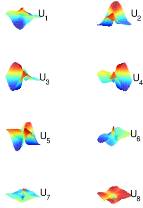
1 ( ) {1... }; k ( ) 0 in P Card k Q Q φ ≈ ∈ < x x . (20)Using a tolerance εKL equal to 0.05 in Equation 6 leads to a K-L decomposition of the sample level-sets in 8 terms and thus 8 random variables have to be identified in this case. The K-L modes corre-sponding to the 8 retained terms are shown in Figure 3.
U1 U2
U3 U4
U5 U6
U7 U8
Figure 3. The K-L modes corresponding to the 8 retained terms of the sample level-sets.
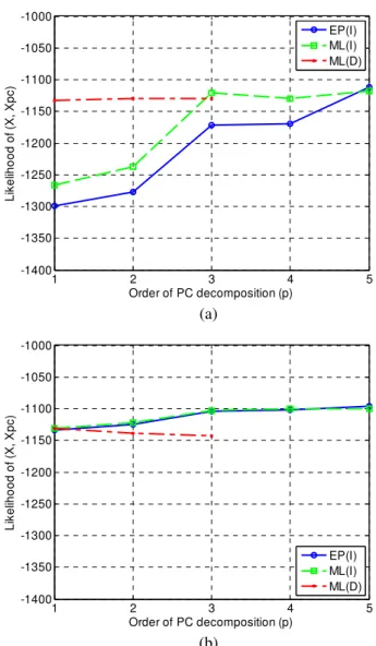
In Figure 4, the values of the pseudo log-likelihood calculated for the initial and identified random vari-ables are plotted as a function of the order p of PC decomposition using the three identification alterna-tives described in sections 4-5 and the two types of PC. Values of the pseudo log-likelihood up to p=3 have been calculated in the case of the maximum likelihood estimation without independence hy-pothesis (denoted as ML(D)) due to the very large computational cost required for higher order PC ex-pansions. For Hermite PC, the results obtained with the maximum likelihood estimation with independ-ence hypothesis (denoted as ML(I)) and the projec-tion method using empirical cumulative distribuprojec-tion functions (denoted as EP(I)) practically coincide. For low order Legendre PC, the ML(D) technique gives better results in likelihood but the results of the two other methods substantially improve as p grows up. This fact implies that the independence assumption is suitable to this problem and has not been strongly affected by the recovery procedure. In the Legendre PC case, the convergence is somewhat slow perhaps due to the complexity of the problem. The marginal pdfs of the first 5 random variables shown in Figure 5 are close to the uniform confirming that the recov-ery procedure was sufficiently accurate. Similar re-sults are obtained with the EP(I) technique and Leg-endre chaos of order p=1 and p=3 for the error in the probability to be inside the hole, presented in Figure 6.
1 2 3 4 5 -1400 -1350 -1300 -1250 -1200 -1150 -1100 -1050 -1000 Order of PC decomposition (p) L ik e lih o o d o f (X , X p c ) EP(I) ML(I) ML(D) (a) 1 2 3 4 5 -1400 -1350 -1300 -1250 -1200 -1150 -1100 -1050 -1000 Order of PC decomposition (p) L ik e lih o o d o f (X , X p c ) EP(I) ML(I) ML(D) (b)
Figure 4. Pseudo log-likelihood values of the initial and identi-fied random variables as a function of the order p of PC de-composition: (a) Legendre chaos, (b) Hermite chaos.
Before closing this section, it can be stated that the two techniques assuming independence are very competitive in terms of accuracy compared to the ML(D) approach, while the projection method EP(I) is the approach having the smallest computational cost for the identification procedure.
-2 0 2 0 1 2 X 1 x P D F (x ) -2 0 2 0 1 2 X 2 x P D F (x ) -2 0 2 0 1 2 X 3 x P D F (x ) -2 0 2 0 1 2 X 4 x P D F (x ) -2 0 2 0 1 2 X 5 x P D F (x ) samples identified
Figure 5. Marginal pdf of the first 5 initial and identified ran-dom variables (Legendre chaos, p=1, EP(I)).
(a) (b)
Figure 6. Error in the probability to be inside the hole (EP(I), Legendre chaos) with (a) p=1 and (b) p=3.
7 CONCLUSIONS
In this paper, an efficient identification procedure of random geometry has been proposed in a form suit-able for numerical simulation within the eXtended Stochastic Finite Element Method (X-SFEM). The method starts from a collection of images represent-ing different outcomes of the random shape to iden-tify. The key-point of the method is to represent the random geometry in an implicit manner using the level-set technique. In this context, the problem of random geometry identification is equivalent to the identification of a random level-set function, which is a random field. This random field is first decom-posed using an empirical Karhunen-Loève expan-sion, which allows representing the samples of the level-set on a reduced basis of deterministic modes. The problem is thus transformed into the probabilis-tic identification of a few random variables, which are the components of the random level-set on this reduced basis of modes. The random variables are represented on a polynomial chaos basis and three efficient numerical strategies are used in order to identify the coefficients of their polynomial chaos decomposition. The performance of these strategies has been evaluated on a "manufactured" random ge-ometry problem using various error criteria. It can be concluded that the two techniques assuming inde-pendence (ML(I) and EP(I)) are very competitive in terms of accuracy compared to the ML(D) approach, while the projection method EP(I) is the approach having the smallest computational cost for the iden-tification procedure. This conclusion is in accor-dance with the assumption of independence which is very often used in practice due to the small collec-tion of images that is usually available.
ACKNOWLEDGEMENT
This work has been supported by the French Na-tional Research Agency (Grant ANR-06-JCJC-0064). This support is gratefully acknowledged.
REFERENCES
Babuška, I., Tempone, R. & Zouraris, G. E. 2005. Solving el-liptic boundary value problems with uncertain coefficients by the finite element method: the stochastic formulation.
Computer Methods in Applied Mechanics and Engineering
194: 1251-1294.
Canuto, C. & Kozubek, T. 2007. A fictitious domain approach to the numerical solution of pdes in stochastic domains.
Numerische Mathematik107(2): 257-293.
Desceliers, C., Ghanem, R. & Soize, C. 2006. Maximum likeli-hood estimation of stochastic chaos representations from experimental data. Int. J. for Numerical Methods in
Engi-neering66(6): 978-1001.
Fang, K.T. & Li, R.Z. 1997. Some methods for generating both an nt-net and the uniform distribution on a Stiefel manifold and their applications. Computational Statistics & Data
Analysis24: 29-46.
Ghanem, R. & Doostan, A. 2006. On the construction and analysis of stochastic models: characterization and propaga-tion of the errors associated with limited data. J. of
Compu-tational Physics217(1): 63-81.
Ghanem, R. & Spanos, P. D. 1991. Stochastic finite elements:
A spectral approach. Springer-Verlag, Berlin, 2nd edition: Dover Publications, NY, 2003.
Nouy, A., Schoefs, F. & Moës, N. 2007. X-SFEM, a computa-tional technique based on X-FEM to deal with random shapes. European J. of Computational Mechanics 16(2): 277-293.
Nouy, A., Clément, A., Schoefs, F. & Moës, N. 2008. An eX-tended Stochastic Finite Element Method for solving sto-chastic partial differential equations on random domains.
Computer Methods in Applied Mechanics and Engineering
197: 4663-4682.
Sethian, J. 1999. Level-set methods and fast marching
meth-ods: Evolving interfaces in computational geometry, fluid mechanics, computer vision and materials science. Cam-bridge University Press, CamCam-bridge, UK.
Soize, C. & Ghanem, R. 2004. Physical systems with random uncertainties: chaos representations with arbitrary probabil-ity measure. SIAM J. on Scientific Computing 26(2): 395-410.
Stefanou, G., Nouy, A. & Clément, A. 2009. Identification of random shapes from images through polynomial chaos ex-pansion of random level set functions, Int. J. for Numerical
Methods in Engineering, in press.
Xiu, D. & Karniadakis, G. E. 2002. The Wiener-Askey poly-nomial chaos for stochastic differential equations. SIAM J.
on Scientific Computing24(2): 619-644.
Xiu, D. & Tartakovsky, D.M. 2006. Numerical methods for dif-ferential equations in random domains. SIAM J. on