Advanced image reconstruction in parallel magnetic resonance imaging : constraints and solutions.

Advanced Image Reconstruction in Parallel Magnetic Resonance

Imaging: Constraints and Solutions

by Ernest N. Yeh

S.B. Electrical Engineering and Computer Science M.Eng. Electrical Engineering and Computer Science

Massachusetts Institute of Technology, 1998

SUBMITTED TO THE HARVARD-MIT DIVISION OF HEALTH SCIENCES AND TECHNOLOGY IN PARTIAL FULFILLMENT OF THE REQUIREMENTS FOR

THE DEGREE OF

DOCTOR OF PHILOSOPHY IN ELECTRICAL AND MEDICAL ENGINEERING

AT THE

MASSACHUSETTS INSTITUTE OF TECHNOLOGY

JUNE 2005

d:c 2005 Massachusetts Institute of Technology. All rights reserved.

Signature of Author:

Harvard-MIT Division of Health Sciences and Technology May 5, 2005

Certified by:

Daniel K. Sodickson, M.D., Ph.D. Assistant Professor of Radiology and Medicine Beth Israel Deaconess Medical Center Harvard Medical School Thesis Supervisor

Accepted by:

Martha L. Gray, Ph.D. Edward Hood Taplin Professor of Medicdal and Electrical Engineering Co-Director, Harvard-MIT Division of Health Science and Technology

MASSACHUSETTS INSUTtIJE OF TECHNOLOGY JUN 302005

IBRARIES

LIBRARIES

II I I I I J ___ . I I I I i I

Advanced Image Reconstruction in Parallel Magnetic Resonance Imaging:

Constraints and Solutions

Ernest N. Yeh

Submitted to the Harvard-MIT Division of Health Sciences and Technology on May 5, 2005 in Partial Fulfillment of the Requirements for the Degree of Doctor of Philosophy in Electrical and Medical Engineering.

ABSTRACT

Imaging speed is a crucial consideration for magnetic resonance imaging (MRI). The speed of conventional MRI is limited by hardware performance and physiological safety measures. "Parallel" MRI is a new technique that circumvents these limitations by utilizing arrays of radiofrequency detector coils to acquire data in parallel, thereby enabling still higher imaging speeds.

In parallel MRI, coil arrays are used to accomplish part of the spatial encoding that was traditionally performed by magnetic field gradients alone. MR signal data acquired with coil arrays are spatially encoded with the distinct reception patterns of the individual coil elements. T[he quality of parallel MR images is dictated by the accuracy and efficiency of an image reconstruction (decoding) strategy. This thesis formulates the spatial encoding and decoding of parallel MRI as a generalized linear inverse problem. Under this linear algebraic framework, theoretical and empirical limits on the performance of parallel MR image reconstructions are characterized, and solutions are proposed to facilitate routine clinical and research applications.

Each research study presented in this thesis addresses one or more elements in the inverse problem, and the studies are collectively arranged to reflect three progressive stages in solving the inverse problem: 1) determining the encoding matrix, 2) computing a matrix inverse, 3) characterizing the error involved. First, a self-calibrating strategy is proposed which uses non-Cartesian trajectories to automatically determine coil sensitivities without the need of an external scan or modification of data acquisition, guaranteeing an accurate formulation of the encoding matrix. Second, two matrix inversion strategies are presented which, respectively, exploit physical properties of coil encoding and the phase information of the magnetization. While the former allows stable and distributable matrix inversion using the k-space locality principle, the latter integrates parallel image reconstruction with conjugate symmetry. Third, a numerical strategy is presented for computing noise statistics of parallel MRI techniques which involve magnitude image combination, enabling quantitative image comparison. In addition, fundamental limits on the performance of parallel image reconstruction are derived using the Cramer-Rao bounds. Lastly, the practical applications of techniques developed in this thesis are demonstrated by a case study in

improved coronary angiography.

ACKNOWLEDGEMENTS

With much joy and humility, I am here to celebrate with each and every one of you whose love, sacrifice and guidance have helped me reach this milestone. This short acknowledgement simply could not convey the many thoughts of mine.

My family has been the greatest blessing in my life. As I was growing up, there was never a single day that I did not feel loved. My parents have taught me the virtue of hard work and optimism. For the twelve years I have been at MIT, my father has worked, without complaints, two full-time jobs to support my education. My mother, who has also made many sacrifices, has nurtured me a relentless passion for education. My big sister, Selina, serving the role of a parent since our immigration to the US, has, through her example, inspired me to pursue my dreams in this land of opportunities.

I have also been blessed by an elite group of colleagues whose intellects are only surpassed by their genialities. My thesis supervisor, Daniel Sodickson, has been instrumental in every aspect during my formative years as a young scientist. He has provided a magical balance of freedom and guidance, allowing me to explore my interests without getting lost. Charles McKenzie, who has taught me everything I know about MR scanners, has also granted me the privileges to work closely with him on many exciting projects. Aaron Grant,

with his vast knowledge about almost every phenomenon in physics, has equally impressive patience in reviewing and offering suggestions to my thesis at various stages. Michael Ohliger, my officemate for five years, has always been the first one to listen to my ideas, and has also devoted many hours in helping refine my thesis.

I would like to express my special gratitude to my thesis committee. David Staelin has been generous in offering his mentorship in multiple occasions. Dave was the course director for a class which I taught as a TA, then served in my PhD qualifying committee, and

now serves in my thesis committee. Rene Botnar, who has taken the trouble to fly back from Germany to attend my defense, has been a wonderful mentor, colleague, and friend. Rene has demonstrated to me how to simultaneously excel in both physics and physique.

There are many friends who have been supportive along the way. William Peake, my undergraduate academic advisor, has continued to be my source of inspiration. BakFun and MeiKee Wong have warmly taken me to their family and provided wisdom and guidance in my searching years. Friends in the MIT Hong Kong Student Bible Study Group, whose heritage and faith I share, have fought side-by-side in many battles of the graduate life. To all of us who are graduating, a job well done!

Last and most importantly, I am inexplicably blessed by my wife, Connie, who has gone through the ups and downs in my graduate years, and is duly credited for giving this thesis document a professional touch. Together, we are thrilled to see the conclusion of my PhD, and ready to embark a new phase of our lives.

This research has been supported by the generosity of the Harvard-MIT Division of Health Sciences and Technology; the National Institutes of Health; and the Whitaker Foundation.

TABLE OF CONTENTS

A cknow led gem ents ...5

Table of C ontents ...

...

...

7

List of Figures ... ...9

List of Tables ... 11

Chapter 1. Introduction ... 13

Section 1.1 General Introduction: Parallel Magnetic Resonance Imaging ... 13

Section 1.2 Statement of the Thesis ... ... ...15

Section 1.3 Background ... 20

Section 1.4 General Summary ... 37

Chapter 2. Self-Calibrating non-Cartesian Parallel Imaging ... 41

Section 2.1 Introduction ...

41

Section 2.2 M ethods ... ... 43

Section 2.3 Results ... 50

Section 2.4 Discussion ...

56

Section 2.5 Conclusions ... 59

Section 2.6 Future Directions .

... 59

Chapter 3. Image Reconstruction with k-space Locality Constraint ... 67

Section 3.1 Introduction ...

67

Section 3.2 Theory ... 69 Section 3.3 M ethods ... 73 Section 3.4 Results ... 75 Section 3.5 D iscussion ... ... ... ...82 Section 3.6 Conclusions ... 88 Section 3.7 Appendix A ... ... 89

Chapter 4. Image Reconstruction using Prior Phase Information ... 95

Section 4.1 Introduction ...

95

Section 4.2 Theory ...

98

Section 4.4 Results ... 108

Section 4.5 Discussion ... 112

Section 4.6 C onclusion s ... ... 114

Chapter 5. Generalized Noise Analysis for Magnitude Image Combination with Parallel M R I ... 119

Section 5.1 Introduction ...

...

119

Section 5.2 Theory ...

...

121

Section 5.3 Methods . ... 129 Section 5.4 R esults ... 131 Section 5.5 Discussion ... 136 Section 5.6 Conclusions ... 139 Section 5.7 Appendix A ... 140 Section 5.8 Appendix B ... 143 Section 5.9 Appendix C ... 145

Chapter 6. Fundamental Limits: Parallel Image Reconstruction as an Array

Processing Technology ...

149

Section 6.1 Introduction ...

149

Section 6.2 Theory ... 151 Section 6.3 Method ... 156 Section 6.4 Results ... 157 Section 6.5 Discussion ... 160 Section 6.6 Conclusions ... 161

Chapter 7. Adaptation of a Cardiac Imaging Technique for Parallel MRI ... 163

Section 7.1 Introduction ...

163

Section 7.2 Methods ... 165

Section 7.3 Results ... 166

Section 7.4 Discussion ... 168

Section 7.5 Conclusions ... 171

Chapter 8. General Discussion and Future Directions ...

175

Section 8.1 Summary of Major Results ... 175

Section 8.2 Future Directions ... 177

LIST OF FIGURES

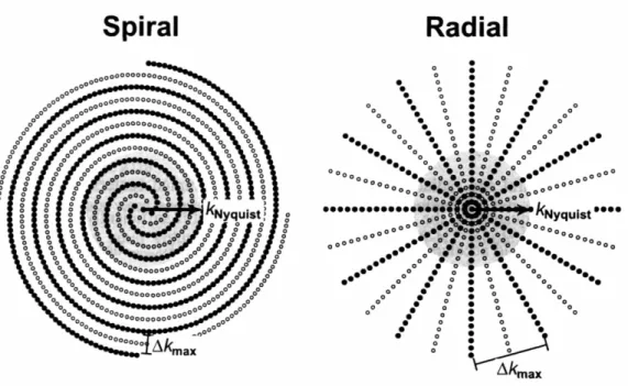
Figure 2.1 Self-Calibrating Spiral and Radial Trajectories ... 46

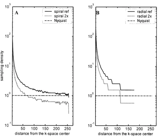
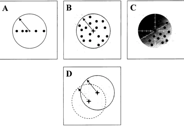
Figure 2.2 Sampling Density of Spiral and Radial Trajectories ... 47

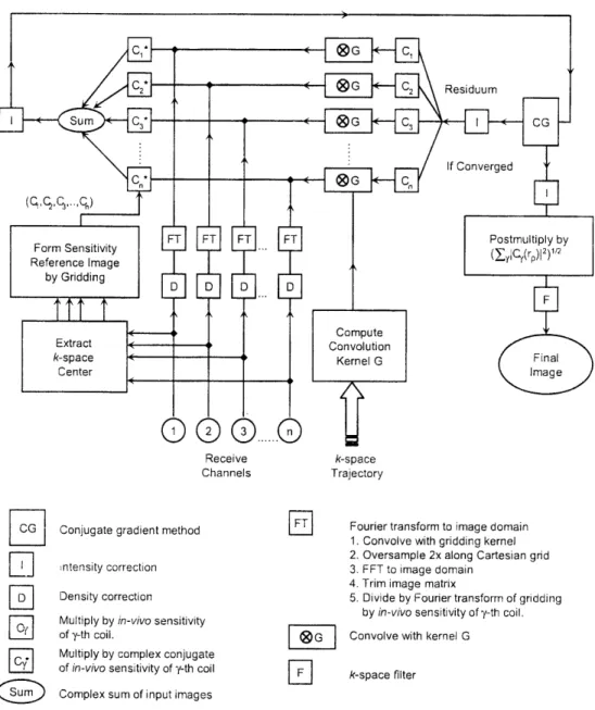
Figure 2.3 Schematic of Self-Calibrating CG-SENSE Algorithm ... 51

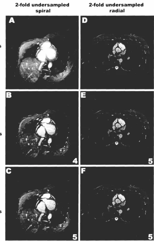
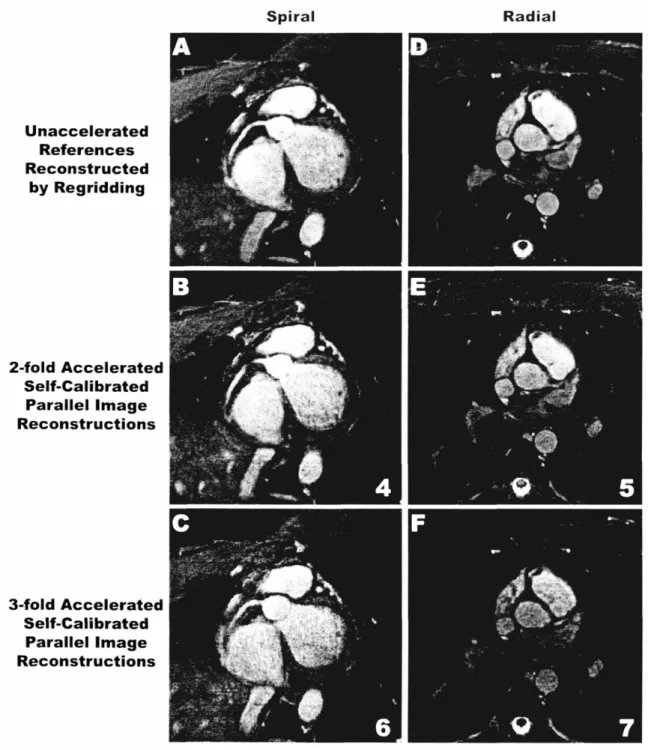
Figure 2.4 2x Self-calibrated and External Calibrated Spiral and Radial Images ... 52

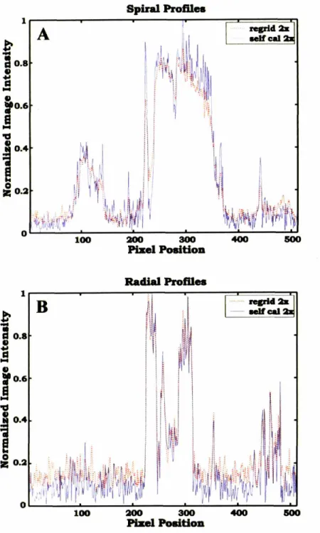
Figure 2.5 Image Intensity Profiles of 2x Spiral and Radial Images ... 54

Figure 2.6 2x and 3x Spiral and Radial Parallel Image Reconstructions ... 55

Figure 3.1 Schematic of the PARS Algorithm ... 70

Figure 3.2 Principle of k-Space Locality in Parallel MRI ... 76

Figure 3.3 Total Error Power vs Sensitivity Noise ... 77

Figure 3.4 Total Error Power vs k-space Radius ... 78

Figure 3.5 In Vivo Image Comparisons of PARS and SENSE ... 80

Figure 3.6 PARS Reconstructions Using Different k-space Radii ... 81

Figure 4.1 Schematic of PARS combined with Phase Constraint ...104

Figure 4.2 Simulations of Partial Fourier Image Reconstructions ... 109

Figure 4.3 Noise in Parallel Image Reconstructions with and without Phase Constraint ... 110

Figure 4.4 Phantom Images from Phase-Constraint Parallel Image Reconstructions ... 111

Figure 4.5 In-Vivo Images from Phase-Constraint Parallel Image Reconstructions ...111

Figure 5.1 Schematic of Sum-of-Squares Combined Parallel Image Reconstruction ...123

Figure 5.2 Probability Density Functions of Perceived Image Intensity ... 131

Figure 5.3 Statistical Biases of Perceived Image Intensity ... 133

Figure 5.4 Image Comparison of Sum-of-Squares PARS Image Reconstructions ...134

Figure 5.5 Comparison of G-factors Obtained by ROI and the proposed Numerical M ethod ... 135

Figure 5.6 Calculated G-factors vs k-space Radius ... 136

Figure 6.1 Schematic of Multiple-Input Multiple-Out (MIMO) Technology ... 150

Figure 6.2 Convergence of Finite-Precision MLE and Full-Matrix Inversion ... 158

Figure 6.3 Error Plots of Finite-Precision MLE ... 159

Figure 7.1 Spiral Coronary MRA Parallel Image Reconstructions ... 167

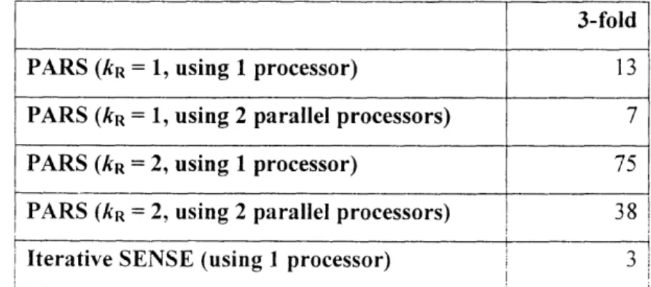
Reconstruction Times (in sec) for Undersampled Cartesian Trajectories ... 79

Reconstruction Times (in min) for Undersampled Spiral Trajectories ... 79

Changes in SNR with Increasing Acceleration Factor for in vivo Data ... 112

Notational Convention for Random Variables ... ... 124

Imaging Parameters for in vivo Spiral Acquisitions ... 165

Imaging Parameters for in vivo Radial Acquisitions ... 166

LIST OF TABLES

Table 3.1 Table 3.2 Table 4.1 Table 5.1 Table 7.1 Table 7.2

CHAPTER 1. INTRODUCTION

SECTION 1.1

General Introduction: Parallel Magnetic

Resonance Imaging

Magnetic resonance imaging (MRI) allows non-invasive diagnostic assessment of the human body without the risk of ionizing radiation. The quality of MR image is critically determined by the imaging speed. However, hardware performance and physiological safety measures have limited the speed of conventional MRI. In recent years, parallel MRI techniques have been developed that utilize radiofrequency (RF) coil arrays to accelerate

image acquisition beyond these previous limits (1-9).

Conventional MRI uses magnetic field gradients to spatially encode the magnetic resonance (MR) signal in order to produce an image with resolution many times finer than the signal wavelength. This so-called Fourier encoding technique, though invented to make MRI possible in the first place (10,11), considerably limits the image acquisition speed, since MR signal data have to be acquired one Fourier component at a time. In 1977, the first clinical MR image of the human body took 5 hours to acquire (12), and nowadays, after almost three decades of research and development, a single MR image can be acquired in less

less reached its imaging speed limit. Even when the most modern conventional scanner hardware is used, cumulative acquisition times may be excessively long for clinical diagnosis that requires datasets of particularly high spatial and temporal resolution. Unfortunately, safety guidelines regarding magnetic field gradient switching and RF power deposition preclude further increases in imaging speed

Prolonged acquisitions are especially problematic for imaging of moving structures such as the heart. Even though several techniques (e.g., breath-holding (13), electrocardiogram gating (14) and diaphragmatic tracking (15)) have been developed to help circumvent the speed bottleneck, accelerating image acquisition remains the most attractive and fundamental solution.

In parallel MRI, RF coil arrays are used to share the burden of spatial encoding that is conventionally accomplished by magnetic field gradients. The spatially varying sensitivities of an RF coil array provide additional encoding of the received MR signal data, and this spatial information permits images to be reconstructed from a small subset of the original Fourier-encoded dataset. In other words, some of the Fourier-encoding steps can be omitted in the image acquisition, consequently accelerating image acquisition. In contrast to the sequential data acquisition scheme in conventional MRI, parallel MRI techniques allow parallel data acquisition via the use of multiple RF detector coils.

Since its first clinical demonstration in 1997 (2), investigators have reported ever increasing acceleration factors, recently up to a factor of 16 in vivo (16). The ability to perform markedly faster MRI not only promises many immediate benefits (e.g., improving image quality, reducing examination time, increasing patient comfort), but also opens up new possibilities (e.g., single breath-hold whole-heart coronary angiography) that were previously

SECTION

1.2 Statement of the Thesis

To date, various challenges in image reconstruction have complicated everyday clinical applications of parallel MRI. This thesis formulates the image reconstruction of parallel MPRI as a generalized linear inverse problem. Under this framework, theoretical and practical limits on the performance of parallel MR image reconstruction are characterized. In particular, :;ix important aspects of parallel MRI are addressed, and practical solutions are proposed to facilitate routine clinical and research applications.

1.2.a Coil Sensitivity Calibration: Accuracy and Consistency

In parallel imaging, MR signal data are spatially encoded using RF coil sensitivities, and parallel image reconstruction requires accurate knowledge of the underlying RF coil reception patterns. RF coils are typically positioned close to the anatomy of interest in order to obtain favorable signal-to-noise ratio. As a result, coil positioning and hence detailed coil sensitivity patterns may change from patient to patient, and potentially from image acquisition to image acquisition, (e.g., as a result of patient motion).

Coil sensitivity information for parallel MR1 can be obtained either from separate reference scans (external calibration) or from reference scans incorporated within the accelerated image acquisitions themselves (self calibration). The use of self-calibrating techniques is attractive since they eliminate the need for additional calibration scans and avoid potential mismatches between calibration scans and subsequent accelerated acquisitions. However, most examples of self-calibrating techniques require modification of data sampling trajectories, potentially limiting the flexibility and the maximum acceleration factor in image acquisitions.

Chapter 2 proposes an inherently self-calibrating image acquisition that makes use of non-Cartesian sampling trajectories. Commonly used non-Cartesian trajectories, namely spiral and radial trajectories, offer inherent self-calibrating characteristics because of their densely sampled centers. At no additional cost in acquisition time and with no modification

sampled central regions of k-space. Illustrative examples are presented to demonstrate feasibility, and physical arguments are put forward to establish the theoretical minimal amount of calibration information required for a successful parallel image reconstruction. Future directions for coil sensitivity calibration are outlined.

1.2.b Computational Efficiency and Stability

After the coil sensitivities are accurately calibrated, parallel MR images can in principle be reconstructed by solving a system of linear equations. However, the system of equations involved is typically prohibitively large for arbitrary sampling trajectories. Efficient algorithms only exist for special cases in which data are sampled on a regularly-spaced Cartesian grid where the Fast Fourier Transform (FFT) can be applied to reduce the computational burden. Even then, the final solution may not be numerically stable, and the numeric instability is especially pronounced in highly accelerated parallel imaging. Together, the computational efficiency and stability represent critical constraints on the performance of parallel MRI, restricting most current applications to relatively low acceleration factors and regular sampling trajectories.

In Chapter 3, the principle of k-space locality is exploited to address some of these computational constraints. An efficient and stable parallel image reconstruction algorithm is proposed: Parallel magnetic resonance imaging with Adaptive Radius in k-Space (PARS). In RF coil encoding, information relevant to reconstructing an omitted datum rapidly diminishes as a function of k-space separation between the omitted datum and the acquired signal data. The proposed PARS method harnesses this principle of k-space locality via a sliding-window approach to judiciously partition the large system of equations into manageable and distributable independent systems of equations, achieving both computational efficiency and numerical stability. Additionally, an empirical method designed to measure total error power is described. The total error power of PARS reconstructions is studied over a range of k-space radii and accelerations, revealing "minimal-error" conditions at comparatively modest k-space radii. For experimental verifications, PARS reconstructions of undersampled in vivo Cartesian and non-Cartesian datasets are shown, and are compared selectively with standard

parallel image reconstructions. Various characteristics of PARS (such as the tradeoff between signal-to-noise ratio and artifact power, and the relationship with iterative parallel conjugate- gradient approaches or non-parallel gridding approaches) are discussed.

1.2.c Phase Constraint: Exploitation of Phase Information for

Parallel MRI

When an image has a slowly spatially-varying phase, conjugate symmetry in k-space allows that image to be reconstructed accurately using only slightly more than half of the data which would otherwise be required. This phase-constrained approach, which can improve image acquisition time by as much as a factor of two, is commonly referred to as half Fourier or, more generally, partial Fourier encoding. Partial Fourier imaging (e.g., Ref. (17)) was clinically implemented for conventional MRI before the invention of parallel MRI. Once parallel imaging techniques became available, it was only natural to combine them with partial Fourier encoding so as to increase imaging speeds still further. However, this combination can also present certain challenges for image reconstruction. Most combinations attempted so far have used sequential concatenations of partial Fourier and parallel image reconstructions. Depending on the particular parallel imaging methods used, and on the order of concatenations, the phase calibration or other conditions for accurate reconstruction may cease to be valid. The lack of mathematical rigor and generality in concatenated approaches could limit their reliablity and robustness for clinical diagnosis.

Chapter 4 presents an integrated image reconstruction approach to combine partial Fourier encoding and parallel imaging. A generalized framework is provided for reconstructing images encompassing either or both techniques and for comparing image quality achieved by varying k-space sampling schemes. The theory of integrated phase-constrained parallel MRI is outlined, and the phase calibration requirements and limitations are discussed. A special derivation is devoted to combining the phase constraint and the k-space locality principle. Simulations, phantom experiments, and in vivo experiments are presented.

1.2.d Error Analysis: Noise in Magnitude Images

Quantitative noise analysis of MR image constructions provides an objective metric to evaluate the performance of a particular image reconstruction approach. However, no noise analysis tool is available for parallel image reconstruction strategies which involve magnitude operations. As a result, comparative noise analysis cannot be performed among these parallel image algorithms, or against other approaches which do not involve magnitude operations.

In general, noise analysis in parallel MRI is different from that of conventional MRI in two critical aspects: First, unlike conventional MRI where noise is uniformly distributed in the reconstructed image, the noise in parallel MR images exhibits significant spatial variation. The signal-to-noise ratio (SNR) can no longer be calculated by a region-of-interest (ROI) approach where the power of noise and signal is estimated in regions that are noise-and dominant, respectively. This ROI method fails because the noise in the signal-dominant region may have different variance than that of in the noise-signal-dominant region. A common method of measuring SNR by taking the quotient of the signal power and the noise power would be potentially incorrect. Secondly, and more importantly, many parallel image algorithms (including those presented in Chapters 3 and 4) involve reconstructing intermediate images and then performing a magnitude combination (e.g., sum-of-squares combinations) to form a final composite image. These magnitude operations transform the underlying noise statistics from Gaussian distributions to distributions not readily characterized in traditional forms.

In Chapter 5, a generalized noise analysis strategy for magnitude-combined parallel image reconstructions is proposed to provide a quantitative metric first to characterize the new noise distribution, and eventually to provide a new basis for comparing different parallel image reconstruction algorithms. It is shown that the new noise distribution can be represented as a linear combination of non-central chi-squares variates. Numeric solutions are outlined for the general case where no closed-form solution exists, and closed-form

1.2.e Theoretical Limits of Parallel Image Reconstruction

The work described in Chapters 2-5 addresses specific aspects of parallel MRI including sensitivity calibration, image reconstruction and noise analysis. While this work and other previous parallel MRI advances have been developed largely within the MRI community,. analogous array processing technologies have also been developed in other disciplines. In fact, the use of detector arrays is common not only in medical imaging such as ultra-sound and multi-detector computerized tomography (MD-CT), but also in non-medical fields such as telecommunications and radio-astronomy. The quest to find fundamental performance limits in parallel image reconstruction has serendipitously led to a convergent path with other array processing technologies. In particular, a close correspondence with multi-input multi-output (MIMO) systems in telecommunications has been reported at a recent conference. Questions have been raised as to whether current parallel image reconstructions are statistically optimal, and if not, whether decoding algorithms in the MIMO system can be used to improve parallel image reconstruction.

Chapter 6 tests the optimality of image reconstruction for parallel MRI by adapting the decoding apparatus used for MIMO. Cramer-Rao bounds for parallel MRI are established. A special case where noise is of Gaussian distribution is explored, and a demonstration of the use of a maximum likelihood decoding algorithm, namely the Viterbi decoding algorithm, is presented. Results from simulations are compared to those predicted by the Cramer-Rao bounds.

1.2.f Adaptation of a Cardiac Imaging Technique to Parallel

MRI

Physiological constraints, e.g. cardiac and respiratory motion, have been a driving force for continual improvement in MR imaging technology. Even though parallel MRI has achieved many-fold accelerations, these physiological constraints are still important considerations in designing imaging protocols. For example, some of the speed gained by parallel MRI may be traded for greater tolerance of heart beat irregularity (cardiac

arrhythmia). It is important to evaluate how the existing clinical imaging protocols could be optimized for use with parallel imaging.

Chapter 7 presents a case study of anatomy-specific clinical applications of parallel MRI. In MR coronary angiography, imaging parameters (e.g., magnetic field gradients, RF excitations and receiver bandwidth) have been designed to work under the timing constraints of conventional MRI. The added flexibility provided by parallel imaging warrants a re-examination of these imaging parameters. Specifically, the study explores the possibility of trading some of imaging speed gain by parallel MRI for increased tolerance for heart rate variability. This study helps conclude the thesis work by demonstrating how a new technological advance can be translated and refined to meet specific clinical needs.

SECTION

1.3 Background

The physical and engineering principles of MRI have been documented in many textbooks (e.g., Ref. (18)). This section is not intended as a comprehensive exposition of MRI. Rather, principles pertinent to the understanding of parallel MRI are reviewed in order to provide a platform for discussion of the dissertation work. A special focus is devoted to spatial encoding and decoding methodologies for conventional and parallel MRI. A formulation of the linear inverse problem for MR image reconstruction is derived, and selected examples of parallel image reconstruction methods are provided.

1.3.a The MR Signal

The MR signal originates from the quantum mechanical phenomenon of nuclear magnetic resonance (NMR). Under the influence of an external magnetic field, the nuclear spins of a given atomic species (e.g., hydrogen nuclei) produce a net equilibrium magnetization Mo given by:

JM(r)= M, (r) i=

B(r)p(r)i

[1.1]

4kBT

Here, r is the 3-dimensional spatial vector, y is the gyromagnetic ratio of the atomic species of interest, h is Planck's constant, k, is Boltzmann's constant, and T is the temperature in degrees Kelvin. B(r) is the magnitude of the external magnetic field, and p(r) is the spin density of the atomic species. The unit vector is parallel to the external magnetic field.

The magnetization vector can be rotated from the z axis by applying a radiofrequency (RF) excitation pulse, resulting in a time-varying magnetization in the transverse plane (x-y plane). The overall effect of the RF excitation is summarized by the flip angle a(r), and the magnetization vector now has a time-dependence, expressed as follows ':

M(r,t)= Mz (r)+ Re[Mx (r)e i(r) (i-i)]

[1.2]

where

M (r)= cos (a(r)) M, (r)

M, (r) = sin (a(r)) M,, (r)

and w(r) is the Larmor frequency at which the nucleus precesses:

c(r)= yB(r).

[1.4]

Finally, the oscillating magnetization vector produces a changing magnetic flux in a nearby RF coil, and the voltage induced around the RF coil can be expressed in terms of a volume integral of .iMxy,

v(t)oc ReL C(r)Mxy (r)ee-(r)ld3r].

[1.5]

Here, the spatially varying C(r) represents the RF reception sensitivity, which is a function of the particular geometry of the coil and its position relative to the magnetization unit. C(r) can be calculated using Maxwell's Equations (or the Biot-Savart law for sufficiently low frequencies) in combination with the principle of reciprocity (19).

IThe rotated magnetization vector reverts to the equilibrium state with the longitudinal and transverse relaxation time constants, T and T₂ respectively. The difference of T and T₂among tissue types can be harnessed to enhance image contrast. However, this topic is beyond the scope of the thesis. In this thesis work, the T and 1'_{2effects are intentionally omitted to better illustrate the issues of spatial encoding in parallel MRI. However,} the generalized framework of this thesis does allow easy incorporation of T and T₂effects in constructing the generalized encoding matrix described in later sections.

The voltage v(t) is subsequently demodulated by cos(wot) and sin(cot), and the results are combined to yield the complex MR signal s(t) as follows,

s(t) = C(r)Mxy,

(r)e-'('(r)-q

)'d3r,

[1.6]

where wo is the demodulation carrier frequency given by:

cw = B, [1.7]

and B is the static component of B(r). (Details about B(r) will be presented later in Eq. [1.19].)

1.3.b Imaging with the MR Signal: Spatial Encoding and Image

Reconstruction

The long wavelength of the MR signal (e.g., 5 m in vacuum at 1.5 Tesla) precludes resolving an object within the image using traditional diffraction methods. Instead, uniquely-identifiable spatial information must be encoded into the MR signal, and the image is reconstructed by properly decoding the spatially-encoded MR signal. After expanding the MR signal equation by substituting Eq., [1.1] into Eq. [1.6],

s(t)= IC(r)sin

(a(r))Mo

(r)e-(w(r)-)'d3r

[1.8]

=

Y2h

2

_{IC(r)sin(a(r))B(r)e-i(B(r)B)(r)d3r}

_[1.8]

4kBT

there are four spatially dependent functions inside the volume integral. Besides the spin density, p(r), which is unknown, the other three functions (i.e., C(r), a(r) and B(r)) are parameters that can be in principle measured a priori. Generally speaking, these three functions reflect spatial encoding at three distinct stages: in the beginning, the RF pulse provides an excitation pattern, a(r); at the end, the MR signal received is weighted by the

coil sensitivity, C(r); in between the RF excitation and the signal reception, the magnetic field, B (r), dictates the phase evolution.2

In the general case where all three functions are used to perform spatial encoding, the spatial encoding function E; (r) may be defined as follows:

Es (r)-

flC(r)sin (a(r))B(r)e

(r)-),

,

[1.9]

where ,l denotes a scalar accounting for the constants outside of the integral of Eq. [1.8]. The discrete-time signal s:

S =S (t), [1.10]

can be interpreted as a generalized projection of p(r) onto E (r) and expressed using the notation of the inner product,

s = (E; (r),p(r)).

[1.11]

A set of basis functions then produces a signal vector with N elements,

S2N

i

E2(r),

(r)

[1.12]

SN2 EN 2 ( r ),

In theory, because p(r) is a continuous function with infinite dimensions, it would require infinitely many projections to perfectly reconstruct p(r). In practice, however, appropriate discretization of the continuous position vector r can be applied to p(r) at selected voxel locations r,, resulting in a column vector p,

Py =P(rr) [1.13]

Eq. [1.12] can now be rewritten using as a matrix equation,

s=Ep

[1.14]

where the entries of the encoding matrix E are:

E:

E

rj.

[1.15]

p can be uniquely reconstructed from N linearly-independent projections, where N equals to the number of voxels. The spatial encoding equations in Eq. [1.14] are central to this thesis work because they immediately cast the image reconstruction problem as a generalized linear inverse problem, which assumes a more familiar form:

b = Ax [1.16]

where b is traditionally the vector of observations, A the known matrix, and x the vector of deterministic unknowns. Different MR image reconstruction algorithms, including those for parallel MRI, may differ in appearance and approaches. Nonetheless, these algorithms achieve the ultimate goal of obtaining a solution of p,

= _{E-'s, [1.17]}

in which they explicitly or implicitly perform the three necessary steps of: a) determining the value of the encoding matrix E, b) computing an inverse E-', and c) minimizing the error

involved.

The remaining sections in this chapter use this linear algebraic framework to characterize the encoding and decoding methodologies which are representative of existing conventional and parallel MRI techniques.

1.3.c Conventional MRI

1.3.c.1

Spatial Encoding Using Magnetic Field Gradients

Conventional MRI relies on the spatially varying magnetic field B(r) in Eq. [1.9] for spatial encoding. A uniform RF excitation pulse is typically applied to rotate the magnetization at a flip angle a(r) = a,. The coil sensitivity C (r) is combined with the spin density p(r) to form the coil-modulated spin density p (r). As a result, the MR signal equation (Eq. [1.8]) is simplified to:

s(t) =4

2

_IfC(r)sin

_{((r))B(r)e-iy(B(r)-B}

_{) p(r)d3r}

4kHT

[1.18]

In most examples of clinical MRI scanners, B(r) is expressed as the sum of the constant external magnetic field B, and linear magnetic field gradients G (r) 3,

B(r)= B, +G(r),

[1.19]

where G (r) can be expressed as the dot product of a gradient vector G with r,

G(r)=G.r

= Gxr, + G,.r + G:rz [1.20]

Moreover, Bo is typically several orders of magnitude greater than G(r), and Eq. [1.18]

becomes, s(t) = y 2 _{sin (,)}

sin(a,))

4k T

B

(r)

e-iy(B(r)-B)

p

(r)

d

3

r

(B

+

G (r))e

- '

_(r)

_{p (r)d}

3

_r.

/h2

sin (a

0)

B

eI(r) pc

(r)d

3

r

4kT

Furthermore, by allowing a time-dependence in G, the phase evolution over time can be expressed in terms of k r where the vector k is defined as,

k=-j

((t)dt.

[1.22]

Eq. [1.21] can be rewritten as:

s(k) =

y2

sin (,,

4kBT

)B

fe

krp (r)d3r.

[1.23] The spatial encoding functions from Eq. [1.9] are simplified as,

3 Nonlinearity of G (r) may occur at the edges of the MR scanner bore, and produce artifacts that can be [1.21]

Ek (r)- ,eikr, [1.24] and the matrix equation for image reconstruction becomes:

s=Ep,.. [1.25]

The encoding functions are Fourier basis functions, and hence this method of spatial encoding is commonly called Fourier encoding. The elements in the signal vector s are the Fourier components of the coil-modulated spin density Pc evaluated at the corresponding "k-space" locations k. An MR dataset is acquired by traversing k-space along various values of k 4, and an image is reconstructed by applying an inverse Fourier transformation on the acquired dataset.

p, = E-'s [1.26]

= InverseFT(s)

In the special cases of regularly sampled k-space trajectories, the fast Fourier transformation (FFT) algorithm can be applied. Additionally, the Fourier transformation is a unitary transformation which provides an optimal noise averaging benefit. Here, the three necessary steps stated in Eq. [1.17] are efficiently accomplished without an explicit effort of determining E, computing E-', or minimizing the error involved.5

1.3.c.2 Field of View and Spatial Resolution

The image information attainable using the Fourier encoding and decoding scheme is summarized as follow: the field of view of the reconstructed image is determined by the k-space inter-sample separation Ak,

Field of View =-,

[1.27]

Ak

and the image spatial resolution is set by the extent of the k-space trajectory kmax 6

4 Particular traversal sequences used in different k-space trajectories (e.g. rectilinear and spiral) are topics in later parts of the thesis.

S Substantial MR engineering efforts have been devoted to the design and building of linear magnetic gradients, so that image reconstruction in conventional MRI can be performed with the ease of FFT.

6 The resolution and the field of view along the principal axes may be independently determined by having different values of kmax and Ak for each axis.

Pixel Size =- [1.28] kmax

For regularly sampled (Cartesian) k-space trajectories, these relationships are rigorously derived from the Nyquist sampling theorem and the discrete Fourier series. First, sampling with an infinite impulse chain (i.e. k = +nAk, n = 0,1,2,..,oo) is equivalent to a periodic replication of the object in the image domain. If the object is of finite length and the

2if

sampling interval in k-space satisfies the Nyquist criterion for Ak < , then the object can be fully reconstructed without aliasing. Second, when a finite impulse chain is used (i.e. k = nAk, and

kl

< kmax), the voxels reconstructed by discrete Fourier representation are no longer ideal delta functions. Instead, they are sinc functions with zero crossings at integral multiples of - , which typically defines the image pixel size.

kmax

For irregularly sampled (non-Cartesian) trajectories, the non-uniform sampling density across k-space makes it difficult to apply the straightforward relationships in Eq. [1.27] to describe the attainable image information content (20). This challenge and its counterpart in parallel MRI will be collectively addressed using the generalized linear inverse

framework later in the thesis.

1.3.c.3 ]Limitations on Conventional MRI Speed

The imaging speed of conventional MRI is primarily limited by the sequential data acquisition scheme implicitly represented by Eqs. [1.22] and [1.24] where the Fourier-encoded data s(k) are acquired one point at a time. To accelerate image acquisition for the same k-space coverage, conventional MRI requires stronger magnetic field gradients, faster gradient switching rates and/or more frequently applied RF pulses (which would result in higher RF power deposition). Unfortunately, any and all of these approaches can pose increasing risks of damaging the underlying biological tissues. In the next section, a safe alternative strategy to accelerate image acquisition is introduced: parallel MRI techniques in which MR data are acquired in parallel via the use of RF coil arrays.

1.3.d Parallel MRI

1.3.d.1 Spatial Encoding Using RF Coil Sensitivities

Parallel MRI techniques make use of RF coil arrays to share the burden of spatial encoding with magnetic field gradients. Individual coil elements have spatially varying sensitivity patterns, and the MR signal equation (Eq. [1.6]) is modified,

s (t) = C,(r) sin (a(r))M,, (r)e(e (r)-)'d3r, [1.29]

where s, (t) represents the MR signal received by the 1h coil with spatial sensitivity C, (r).

The values of C, (r) can be determined a priori using calibration data, which will be described later in the chapter. Other than the multi-coil detection, the data acquisition scheme in parallel MRI is similar to that of conventional MRI: a uniform RF excitation pulse is initially applied to rotate the net magnetization by a constant flip angle ao, and magnetic field gradients are used to traverse kspace. In analogy to the steps taken in Eqs. [1.21] -[1.25], the MR signal equation for parallel imaging can be expressed as:

s (k)= I

sin(

0

)B,

eIkrC, (r)p(r)d

3

r

[1.30]

4k T

and the spatial encoding functions are defined as follows:

Ek,l (r)- l3C, (r)ek . [1.31] where the scalar 6 accounts for the constants outside the integral in Eq. [1.31]. Here, the MR signal is seen as a generalized projection of spin density onto the hybrid encoding function of magnetic field gradients and coil sensitivity. The extra index in Ekt signifies that the

number of encoding functions has increased by a factor equal to the number of array elements, L.

1.3.d.2 Acceleration in Imaging Speed

If a dataset acquired with a one-coil system is sufficient to reconstruct an image, then using an identical sampling trajectory in k-space, a dataset acquired with a multi-coil system must contain redundant spatial information. In the framework of the generalized linear inverse problem, the number of equations is increased by a factor of L while the number of

unknowns remains the same. The matrix system is overdetermined. In parallel imaging, this redundancy in spatial encoding is exploited to allow image acceleration. The k-space trajectory only needs to traverse a subset of the original k-space locations, resulting in a proportionally faster acquisition.

In principle, if there are a very large number of coil elements each with distinct sensitivity, the spatial encoding using magnetic field gradients can be omitted altogether. In such a scenario, MRI would be nearly instantaneous. In practice, the complementary use of magnetic field gradients is still desirable and necessary for reasons that will become apparent.

1.3.d.3 Parallel Image Reconstruction Methods

Image reconstruction in parallel MRI, like the generalized linear inverse framework represented in Eqs. [1.16] and [1.17] , can also be divided into three steps: a) calibration for the encoding matrix E; b) computing an inverse E-'; c) minimizing the error involved in the reconstructi on.

1.3.d.3.1 Sensitivity Calibration to Obtain the Encoding Matrix E

COIL SENSITIVITY MAPS

Knowledge of the coil sensitivities C, (r) is required to formulate the encoding functions (Eq. [1.31]) which collectively constitute the encoding matrix E. These coil sensitivities can in principle be calculated if the coil array geometry and location are known. In practice, however, for flexible coil arrays whose positions vary from scan to scan, the coil sensitivity information is preferably recalibrated each time. The coil sensitivities can be calibrated from coil-modulated images p, (r), where

p (r)= C, (r) p(r)

[1.32]

is obtained using conventional MRI acquisition and image reconstruction methods (Eq. [1.26]). These coil images may have lower spatial resolution (i.e., smaller kmax in Eq. [1.28]

) than the accelerated diagnostic images, but are required to have a sufficient field-of-view (i.e., large enough Ak in Eq. [1.27]) to satisfy the Nyquist criterion. To eliminate the spin density component in p, (r), an additional image can be acquired using a bird-cage body coil which is designed to have a uniform RF spatial reception field, Cbod_,cojl (r) = CO. A quotient

is performed between the two coil images to obtain a scaled version of C, (r),

p,(r)

C (r)p(r)

1

Pbody-coai

(r)

Cbo,dco,,

(r)

p(r)

C,(r)

[1.33]

If a body-coil image is not available, a sum-of-squares combined image can be used to divide out the spin density,

p,(r)

C, (r)p(r)

1

(r

[1.34]

p

~

(r) 22

C[1.34]

Since the multiplication of is common to all coils, it can be incorporated in the /IIc, (r)1

formulation of an effective encoding function which differs from the original encoding function (Eq. [1.31 ]) as follows:

Ek,

(r)

=

Ekt

(r)

[1.35]

The effective spin density reconstructed by parallel MRI is expressed as,

/(r)=

,C

C,(r)1

2_{p(r). [1.36]}

An interesting property is illustrated here that an arbitrary function can be used in lieu of , and p(r) can be obtained by performing a multiplication of the same

,

,

(r)l2

EXTERNAL SENSITIVITY CALIBRATION AND SELF-CALIBRATION

Calibration data, which are used to reconstruct the coil images in Eq. [1.32], can be obtained from a separate scan before or after the image acquisition. Because of the requirement of external information, this approach is generally known as external calibration. Alternatively, the calibration scan can be incorporated as a part of the image acquisition, and the calibration data can be extracted from the image dataset. This approach is called auto-calibration or self-auto-calibration7. The crucial difference between the external- and self-calibration approaches lies in the timing of the acquisition of self-calibration data relative to the image acquisition. These differences are discussed in detail in Chapter 2.

1.3.d.3.2 Image Reconstruction: Computing a Matrix Inverse E-1

Various parallel image reconstruction algorithms have been developed to solve the generalized linear inverse problem, and Sodickson et al has shown the linkage between some of the different approaches (7). Here, three major classes of parallel image reconstructions (full matrix inversion, k-space block-diagonalization, and image-domain block-diagonalization) are discussed with frequent reference to the central equation: s = Ep.

FULL MATRIX INVERSION

The full matrix inversion approach entails a straightforward inversion of Eq. [1.14], finding a matrix inverse E-' such that E-'E = I and thus,

Precon = E-'s, [1.37] where I is an identity matrix. When the image acceleration factor is equal to the number of array elements L, then the encoding matrix E is square, and E-' is uniquely determined. Often, however, the acceleration factor is less than L. E is rectangular with more rows than columns, and the matrix system is overdetermined. E- is no longer unique. Instead, the Moore-Penrose pseudo-inverse is used to provide a least-squares solution:

7 For self-calibrating parallel MRI, methods exist that allow coil sensitivity calibration without explicitly reconstructing the calibration images. These methods however generally observe calibration requirements

E-' = (EHE) EH [1.38]

where the superscript (.)H denotes Hermitian conjugation. (This equation must be modified slightly to minimize error in the presence of noise correlations between array elements: see Section 1.5.c.3 to follow.) While it may be numerically unstable and computationally intensive to calculate the pseudo-inverse, the full matrix inverse approach has the appeal of a theoretically exact solution. Notable representatives of this approach include Subencoding (1), SENSE (3), Space-RIP (4) and GEM (7).

k-SPACE BLOCK-DIAGONALIZATION

SMASH and its derivatives rely on a different approach to matrix inversion using k-space block-diagonalization. In the k-k-space block-diagonalization approach, the encoding matrix E is first Fourier transformed to become EF7T, where EF7 = EF and F denotes a Fourier transformation matrix. Coil sensitivities are in general band-limited -a property that will be more fully explored later in the thesis - and as a result, the matrix EFT is approximately band-diagonal. An inverse (EFT ) k can be determined efficiently by applying either block-by-block inversion or sparse matrix techniques. E-l can be obtained by performing another Fourier transformation as follows,

E = EFF-'

E-l =(EFF-I - [1.39] [1.39]

=F(EF)-'

= F (Er )block-diag

The block-by-block inversion, while providing the advantages of numerical stability and computational efficiency, makes the inversion inexact,

E-'E I.

[1.40]

Tradeoffs between inexactness (artifact) and numerical stability will be an important subject in later chapters. Notable representatives of this k-space block-diagonalization approach include SMASH (2), GRAPPA (8), ASP (21), hybrid GEM (7), and generalized SMASH (9).

IMAGE-DOMAIN BLOCK-DIAGONALIZATION

A third approach to parallel image reconstruction is more restrictive than the other two, but it is included here in order to facilitate discussions in Chapter 6 where correspondence between parallel MRI and wireless communications is made. In the image-domain block-diagonalization approach, the coil sensitivity Cl (r) is assumed to have limited spatial extent, and beyond some distance nn,,,,ledFOV from r, the value of C, (r) drops below

a threshold value ChresoId

C, (r, + Ar) < Clhreshold for IArl > 1inlJ-FOV [1.41] and ,mirnd-edJ1. O< Aifull-FOV. As a result of the smaller field of view, the k-space sampling can be more sparsely without incurring aliasing. The coil images may be independently reconstructed as in conventional MRI, and are then combined after being appropriately shifted according to their center position r. PILS is a representative of this image-domain block-diagonal approach (5).

1.3.d.3.3 Parallel MRI Error Estimation and Quantification

ERROR IN PARALLEL IMAGE RECONSTRUCTION

In general, there are two types of errors in parallel MR image reconstruction. The first type involves systematic errors that may result from an inaccurate coil sensitivity calibration or an inexact image reconstruction such as the block-diagonalization approaches. It is difficult to quantify these errors since they depend on sporadic events (e.g., sudden motion of the patient which shifts the coil arrays), or are related to the tradeoff between image artifact and signal-to-noise in an inexact reconstruction. These will be discussed more thoroughly in Chapters 3 and 5.

The second type of error is statistical error due to propagation of noise, and algorithms have been developed to minimize this type of error. In MR signal detection, noise manifests itself as a statistical fluctuation of voltage across the terminals of an RF coil, and the underlying stochastic process can be characterized experimentally. In practice, noise at a

typically correlated, and noise covariance matrix 'P can be defined where the entry ,, is the noise correlation between coils and '. The overall noise covariance matrix for the signal vector s can be expressed as:

'=P

®Idk, [1.42]

where the direct product with the identity, Idk, indicates replication for all k-space indices.

NOISE IN THE MR IMAGE

In parallel MR images reconstructed using the full matrix inversion, the image noise covariance A can be expressed in terms of the encoding matrix inverse E-' and the signal noise covariance matrix I,

A = (E-')

v

(E-)' .

[1.43]

To achieve minimize noise covariance in the final image, noise decorrelation can be first performed on the MR signal, sec,rr = L-'s and the encoding matrix E ecorr = L-'E where the

lower triangular matrix L is obtained from Cholesky decomposition of P,

P= LLH. [1.44]

The minimum-variance version of Eq. [1.38] is,

Eminvar = (EcorEdcrr )-I Ecor r

= ((L'E)H (L'E))-' (L-E)H [1.45] = (EH-'E)-IEH (L' )H

and the new image noise variance matrix in the final image is,

invar :((Edecorr E) ao,r

)

d((Edecor

)

Edcor

deorr orr [1.46]

((EEd)H

(L-'E)[1.46]

=

((L'E)

(L-E))

=(EH-'E)-'

Preconstructed =EinvarSde.orr ={(E v E)l E HI

}s.

[1.47] An important note should be made that the example shown here involves only linear operations. When the parallel image reconstruction involves non-linear operations (such as magnitude combination), the noise variance is no longer defined within traditional metrics, and thus will require new methods such as the one proposed in Chapter 5.

NOISE AMPLIFICATION IN PARALLEL

MRI

Noise metrics have been developed for parallel imaging techniques whose noise characteristics have been characterized by Eq. [1.43]. These metrics typically focus on the amplification of noise in an image reconstructed from an undersampled dataset compared to that of a fully-sampled reference dataset. The noise variance in an image voxel, y, is given by the diagonal element of A,

02

= Awt, [1.48]

and a noise amplification factor, g-factor, is defined as

/.-_! 1 SNRr4

9=g

Hi

=

a

SN

"[1.49] g= 1.2 R -R SNR₀,.,₁'

where 0,e, and -ef are the noise variances in the parallel and conventional MR images respectively, and R is the image acceleration factor between the parallel and reference images. In general, the decrease in SNR in a parallel MR image reconstruction is due two factors: the inherent loss of noise averaging due to the reduction of data samplings and the non-orthogonality of RF coil encoding. For example, the Fourier encoding functions in conventional MRI are orthogonal, allowing a unitary matrix inversion with optimal noise averaging. However, the generalized encoding functions in parallel MRI are not orthogonal because of the overlapping of broad coil sensitivities. As a result, the matrix inversion in parallel image reconstruction is no longer unitary. Only in the ideal case when the coil sensitivities are perfectly orthogonal would g-factor reach the theoretical lower bound of 1. In practice, the g-factor provides an internal assessment of the spatial encoding capability of a particular RF coil array. However, a more definitive assessment is to evaluate the absolute

SNR (or noise variances) of the image reconstruction. Paradoxically, a coil array carefully optimized for g-factor may yield a lower absolute SNR than an array whose g-factor is otherwise not optimized.

1.3.e Transmit Encoding

SPATIAL ENCODING WITH SPATIALLY-SELECTIVE RF PULSES

The remaining spatially-varying term in Eq. [1.6] is the flip angle a(r). This component does not provide an immediate benefit of accelerating image acquisition, and parallel MRI until recently has not incorporated this component. In fact, this thesis work assumes spatially uniform RF excitations. A portion of Chapter 7 proposes a strategy involving the use of various flip angles, but it is not intended for the purpose of spatial encoding. For the interest of completeness and also for future directions of MRI, it is important to note the potential of using RF pulses to performing additional spatial encoding.

Volume-selective RF pulses are commonly used to provide uniform excitation within a volume V,

{a,

forrE V

a(r) ao,, for re V [1.50] 0, otherwise j

More complex excitation patterns can be achieved by using appropriate combinations of RF and gradient waveforms, or else by using RF coil arrays to transmit. Active research is exploring the expansion of spatial encoding capabilities to realize a full complement of encoding functions:

Eki ,m

(r) - fsin (

m

(r))C, (r)e

- k

r

.

[1.51]

Here, the added index m denotes the different excitation patterns that can be applied at different time points (22), or else in different excitation coils (23,24). The number of basis functions in the new encoding matrix E, as well as its over-determinacy, has increased by a factor of m. When the extra encoding is applied at different time points, it comes at a cost of increasing the acquisition time by the same factor, but this approach may be used to tailor encoding functions so as to provide numerical stability that is not achievable otherwise.

When the extra encoding is applied using arrays of transmit coils, the duration of RF pulses and or the RF power deposition may be reduced for any given pulse profile (this approach is commonly referred to as "Transmit Parallel Imaging.") An in-depth exposition of the full potential of spatially varying RF excitation is beyond the scope of this dissertation. Nevertheless, the last dimension in MR spatial encoding and decoding is an important subject

for ongoing research (23,24).

SECTION

1.4 General Summary

The organization of the thesis can be best presented in relation to the generalized linear inverse problem. Chapters 2-7, though designed to be individually self-contained, are collectively arranged in logical sequence to address the different elements of the inverse problem. Chapter 2 establishes an accurate and robust method for measuring E. Chapter 3 proposes an efficient algorithm to invert E based on a special RF encoding characteristic. Chapter 4 focuses on a physical property of p that facilitates the matrix inversion. Chapter 5 analyzes the effects of noise and systematic errors on the reconstruction of p. Chapter 6 derives the theoretical limits on the overall inverse problem s = Ep. Chapter 7 reports a practical case study in clinical cardiac imaging using the techniques developed in this thesis.

Chapter 1 References

1. Ra JB, Rim CY. Fast imaging using subencoding data sets from multiple detectors. Magn Reson Med 1993;30(1):142-5.

2. Sodickson DK, Manning WJ. Simultaneous acquisition of spatial harmonics (SMASH): fast imaging with radiofrequency coil arrays. Magn Reson Med

1997;38(4):591-603.

3. Pruessmann KP, Weiger M, Scheidegger MB, Boesiger P. SENSE: sensitivity encoding for fast MRI. Magn Reson Med 1999;42(5):952-62.

4. Kyriakos WE, Panych LP, Kacher DF, Westin CF, Bao SM, Mulkern RV, Jolesz FA. Sensitivity profiles from an array of coils for encoding and reconstruction in parallel (SPACE RIP). Magn Reson Med 2000;44(2):301-8.

5. Griswold MA, Jakob PM, Nittka M, Goldfarb JW, Haase A. Partially parallel imaging with localized sensitivities (PILS). Magn Reson Med 2000;44(4):602-9. 6. McKenzie CA, Yeh EN, Sodickson DK. Improved spatial harmonic selection for

SMASH image reconstructions. Magn Reson Med 2001;46:831-836.

7. Sodickson DK, McKenzie C. A generalized approach to parallel magnetic resonance imaging. Med Phys 2001;28(8): 1629-1643.

8. Griswold MA, Jakob PM, Heidemann RM, Nittka M, Jellus V, Wang J, Kiefer B,

Haase A. Generalized autocalibrating partially parallel acquisitions (GRAPPA). Magn Reson Med 2002;47(6):1202-10.

9. Bydder M, Larkman DJ, Hajnal JV. Generalized SMASH imaging. Magn Reson Med 2002;47(1):160-70.

10. Lauterbur P. Image formation by induced local interactions: Examples employing NMR. Nature 1973;242:190.

11. Mansfield P, Grannell PK. NMR 'diffraction' in solids. J Phys C: Solid State Phys 1973;6:L422.

12. Damadian R, Goldsmith M, Minkoff L. NMR in cancer: XVI. FONAR image of the live human body. Physiol Chem Phys 1977;9(1):97-100, 108.

13. Bloomgarden DC, Fayad ZA, Ferrari VA, Chin B, Sutton MG, Axel L. Global cardiac function using fast breath-hold MRI: validation of new acquisition and analysis techniques. Magn Reson Med 1997;37(5):683-92.

14. Glover GH, Pelc NJ. A rapid-gated cine MRI technique. Magn Reson Annual 1988:299.

15. Ehman RL, Felmlee JP. Adaptive technique for high-definition MR imaging of moving structures. Radiology 1989; 173(1):255-63.

16. Zhu Y, Hardy CJ, Sodickson DK, Giaquinto RO, Dumoulin CL, Kenwood G, Niendorf T, Lejay H, McKenzie CA, Ohliger MA and others. Highly parallel volumetric imaging with a 32-element RF coil array. Magn Reson Med 2004;52(4):869-77.

17. Margosian P, Schmitt F, Purdy DE. Fast MR imaging: Imaging with half the data. Health Care Instrum 1986; 1:195-7.

18. Haacke EM, Brown RW, Thompson MR, Venkatesan R. Magnetic Resonance Imaging: Physical Principles and Sequence Design: Wiley & Sons; 1999.

19. Hoult DI, Chen CN, Sank VJ. The field dependence of NMR imaging. II. Arguments concerning an optimal field strength. Magn Reson Med 1986;3(5):730-46.

20. Pipe JG. Reconstructing MR images from undersampled data: data-weighting considerations. Magn Reson Med 2000;43:867-875.

21. Lee RF, Westgate CR, Weiss RG, Bottomley PA. An analytical SMASH procedure (ASP) for sensitivity-encoded MRI. Magn Reson Med 2000;43(5):716-725.

22. Kyriakos WE, Panych LP. Optimization of Parallel Imaging By Use of Selective Excitation. In: Proc 9th Annual Meeting ISMRM, Glasgow, Scotland, UK, 2001. p 768.

23. Katscher U, Bornert P, Leussler C, van den Brink JS. Transmit SENSE. Magn Reson Med 2003;49(1): 144-50.

24. Zhu Y. Parallel excitation with an array of transmit coils. Magn Reson Med 2004;51(4):775-84.

CHAPTER 2. SELF-CALIBRATING

NON-CARTESIAN PARALLEL IMAGING

8

Image reconstruction for parallel MRI has been formulated in Chapter 1 as a linear inverse problem,

s=Ep, [2.1]

where the observation vector s corresponds to the MR signal acquired, the matrix E the generalized MR encoding matrix, and the unknown vector p the spin density of interest. This chapter is devoted to the development of an inherently self-calibrating strategy to determine

E.

SECTION

2.1 Introduction

The accuracy of coil sensitivity estimates is a major determinant of the quality of parallel magnetic resonance image reconstructions. While the level of tolerance for sensitivity rniscalibration differs from technique to technique, any significant discrepancy in coil sensitivity references introduces systematic errors in reconstructed images while

8 The work in this chapter has been adapted for publication as "Yeh EN, Stuber M, McKenzie CA, Botnar RM, Leiner T, Ohliger MA, Grant AK, Willig-Onwuachi JD, Sodickson DK. Inherently Self-Calibrating