HAL Id: hal-00610637
https://hal.archives-ouvertes.fr/hal-00610637v2
Submitted on 24 Oct 2011
HAL is a multi-disciplinary open access
archive for the deposit and dissemination of
sci-entific research documents, whether they are
pub-lished or not. The documents may come from
teaching and research institutions in France or
abroad, or from public or private research centers.
L’archive ouverte pluridisciplinaire HAL, est
destinée au dépôt et à la diffusion de documents
scientifiques de niveau recherche, publiés ou non,
émanant des établissements d’enseignement et de
recherche français ou étrangers, des laboratoires
publics ou privés.
eigen-modes in a normally magnetized nano-pillar
Vladimir V. Naletov, G. de Loubens, Gonçalo Albuquerque, Simone
Borlenghi, Vincent Cros, Giancarlo Faini, Julie Grollier, Hervé Hurdequint,
Nicolas Locatelli, Benjamin Pigeau, et al.
To cite this version:
Vladimir V. Naletov, G. de Loubens, Gonçalo Albuquerque, Simone Borlenghi, Vincent Cros, et al..
Identification and selection rules of the spin-wave eigen-modes in a normally magnetized nano-pillar.
Physical Review B: Condensed Matter and Materials Physics (1998-2015), American Physical Society,
2011, 84 (22), pp.224423. �10.1103/PhysRevB.84.224423�. �hal-00610637v2�
magnetized nano-pillar
V.V. Naletov,1, 2 G. de Loubens,1,∗ G. Albuquerque,3 S. Borlenghi,1 V. Cros,4 G. Faini,5 J. Grollier,4 H.
Hurdequint,6N. Locatelli,4 B. Pigeau,1A. N. Slavin,7 V. S. Tiberkevich,7 C. Ulysse,5 T. Valet,3 and O. Klein1,†
1
Service de Physique de l’ ´Etat Condens´e (CNRS URA 2464), CEA Saclay, 91191 Gif-sur-Yvette, France
2
Physics Department, Kazan Federal University, Kazan 420008, Russian Federation
3
In Silicio, 730 rue Ren´e Descartes 13857 Aix En Provence, France
4
Unit´e Mixte de Physique CNRS/Thales and Universit´e Paris Sud 11, RD 128, 91767 Palaiseau, France
5
Laboratoire de Photonique et de Nanostructures, Route de Nozay 91460 Marcoussis, France
6
Laboratoire de Physique des Solides, Universit´e Paris-Sud, 91405 Orsay, France
7
Department of Physics, Oakland University, Michigan 48309, USA
(Dated: October 24, 2011)
We report on a spectroscopic study of the spin-wave eigen-modes inside an individual normally
magnetized two layers circular nano-pillar (Permalloy∣Copper∣Permalloy) by means of a Magnetic
Resonance Force Microscope (MRFM). We demonstrate that the observed spin-wave spectrum crit-ically depends on the method of excitation. While the spatially uniform radio-frequency (RF)
magnetic field excites only the axially symmetric modes having azimuthal index ℓ= 0, the RF
cur-rent flowing through the nano-pillar, creating a circular RF Oersted field, excites only the modes
having azimuthal index ℓ = +1. Breaking the axial symmetry of the nano-pillar, either by tilting
the bias magnetic field or by making the pillar shape elliptical, mixes different ℓ-index symmetries, which can be excited simultaneously by the RF current. Experimental spectra are compared to theoretical prediction using both analytical and numerical calculations. An analysis of the influence of the static and dynamic dipolar coupling between the nano-pillar magnetic layers on the mode spectrum is performed.
I. INTRODUCTION
Technological progress in the fabrication of hybrid nanostructures using magnetic metals has allowed the emergence of a new science aimed at utilizing spin depen-dent effects in the electronic transport properties1. An
elementary device of spintronics consists of two magnetic layers separated by a normal layer. It exhibits the well-known giant magneto-resistance (GMR) effect2,3, that is,
its resistance depends on the relative angle between the magnetic layers. Nowadays, this useful property is ex-tensively used in magnetic sensors4,5. The converse
ef-fect is that a direct current can transfer spin angular momentum between two magnetic layers separated by either a normal metal or a thin insulating layer6,7. As a
result, a spin polarized current leads to a very efficient destabilization of the orientation of a magnetic moment8.
Practical applications are the possibility to control the digital information in magnetic random access memo-ries (MRAMs)9,10 or to produce high frequency signals
in spin transfer nano-oscillators (STNOs)11,12.
From an experimental point of view, the precise iden-tification of the spin-wave (SW) eigen-modes in hybrid magnetic nanostructures remains to be done13–18. Of
particular interest is the exact nature of the modes ex-cited by a current perpendicular-to-plane in STNOs. Here, the identification of the associated symmetry be-hind each mode is essential. It gives a fundamental insight about their selection rules and about the mu-tual coupling mechanisms that might exist intra or in-ter STNOs. It also dein-termines the optimum strategy to couple to the auto-oscillating mode observed when the
spin transfer torque compensates the damping, a vital knowledge to achieve phase synchronization in arrays of nano-pillars19. These SW modes also have a
fundamen-tal influence on the high frequency properties of these de-vices and in particular on the noise of magneto-resistive sensors20,21.
A natural mean to probe SW modes in hybrid nanos-tructures is to use their magneto-resistance properties. For instance, thermal SW can be directly detected in the noise spectrum of tunneling magneto-resistance (TMR) devices owing to their large TMR ratio22,23. It is also
pos-sible to use spin torque driven ferromagnetic resonance (ST-FMR)24–30. In this approach, an RF current
flow-ing through the magneto-resistive device is used to excite the precession of magnetization and to detect it through a rectification effect. Direct excitation of SW modes by the RF field generated by micro-antennas and their de-tection through dc rectification31or high-frequency GMR
measurements32has also been reported in spin-valve
sen-sors. In all these experiments, the static magnetiza-tions in the spin-valve have to be misaligned in order for the magnetization precession to produce a finite volt-age. Because highly symmetric magnetization trajecto-ries do not produce any variation of resistance with time in some cases, a third magnetic layer playing the role of an analyzer can be introduced33. In ST-FMR, the
non-collinearity of the magnetizations is also required for the RF spin transfer excitation not to vanish25,26.
More-over, the latter was never directly compared to standard FMR, where a uniform RF magnetic field is used to ex-cite SW modes. Thus, although the voltage detection of SW eigen-modes in hybrid nanostructures is elegant, one
should keep in mind that some of them might be hidden due to symmetry reasons.
Here, we propose an independent method of detect-ing the magnetic resonance inside a spin-valve nanostruc-ture. We shall use a Magnetic Resonance Force Micro-scope (MRFM)34–38. A first decisive advantage of the
MRFM technique is that the detection scheme does not rely on the SW spatial symmetry because it measures the change in the longitudinal component of the magne-tization. Like a bolometric detection, mechanical based FMR detects all the excited SW modes, independently of their phase39,40. A second decisive advantage is that
MRFM is a very sensitive technique that can measure the magnetization dynamics in nanostructures buried under metallic electrodes41–43. Indeed, the probe is a magnetic
particle attached at the end of a soft cantilever and is coupled to the sample through the dipolar interaction.
In our roadmap to characterize the nature of the auto-oscillation modes in STNOs, we report in this work on a comprehensive identification of the SW eigen-modes in the simplest possible geometry: the normally mag-netized circular spin-valve nano-pillar. This configura-tion is obtained by saturating the device with a large external magnetic field oriented perpendicular to the lay-ers. Thanks to the preserved axial symmetry, a simpli-fied spectroscopic signature of the different SW eigen-modes is expected. This identification is achieved exper-imentally from a comparative spectroscopic study of the SW eigen-modes excited either by an RF current flow-ing perpendicularly through the nano-pillar, as used in ST-FMR, or by a homogeneous RF in-plane magnetic field, as used in conventional FMR. It shall be developed as follows. In section II, we present the MRFM setup and the experimental protocol used to perform SW spec-troscopy in a spin-valve. We show that the SW spectrum excited by a homogeneous RF magnetic field is distinct from the SW spectrum excited by an RF current flowing through the nano-pillar. In section III, we perform unam-biguous assignment of the resonance peaks to the differ-ent layers by experimdiffer-ental means. We determine which layer contributes mostly to the observed resonant signals by adding a direct current through the nano-pillar, that produces opposite spin transfer torques on each magnetic layer. In section IV, we analyze the spectra by theoret-ical means using both a two-dimensional analyttheoret-ical for-malism and a three-dimensional micromagnetic simula-tion package, SpinFlow 3D. By careful comparison of the measured spectra to the calculations, the nature of the SW dynamics in the system is identified and the selec-tion rules for SW spectroscopy in perpendicularly mag-netized spin-valve nanostructures are established. This result is completed in section V by a study of the influ-ence of symmetry breaking on the selection rules. This is obtained experimentally by introducing a tilt angle of the applied magnetic field, and in simulations by chang-ing the shape of the nano-pillar. In the conclusion, we emphasize the importance of this work for phase syn-chronization of STNOs. The paper is arranged in such
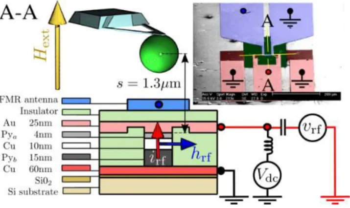
FIG. 1. (Color online) Schematic representation of the exper-imental setup used for this comparative spin-wave spectro-scopic study. The magnetic sample is a circular nano-pillar
comprising a thin Pya and a thick Pyb magnetic layers
sep-arated by a Cu spacer. It is saturated by a large magnetic
field Hext applied along its normal axis. A cantilever with
a magnetic sphere attached at its tip monitors the magne-tization dynamics inside the buried structure. The inset is a microscopy image (top view) of the two independent ex-citation circuits: in red the circuit allowing the injection of an RF current perpendicular-to-plane through the nano-pillar (irf, red arrow); in blue the circuit allowing the generation of
an RF in-plane magnetic field (hrf, blue arrow). The
nano-pillar is at the center of the yellow cross-hair. The main figure
is a section along the A− A direction.
a fashion so as to present the main results in the body of the text. A comprehensive appendix has been put at the end of the paper, where the details of the introduced material are developed.
II. FERROMAGNETIC RESONANCE FORCE
SPECTROSCOPY
This section starts with a description of the nano-pillar sample, followed by a description of the MRFM instru-ment used for this spectroscopic study. Then, we com-pare the experimental SW spectra excited by an RF cur-rent flowing perpendicularly through the nano-pillar, as used in ST-FMR, and by a uniform RF magnetic field applied parallel to the layers, as used in standard FMR.
A. The lithographically patterned nanostructure
The spin-valve structure used in this study is a stan-dard Permalloy (Ni80Fe20=Py) bi-layer structure
sand-wiching a 10 nm copper (Cu) spacer: the thicknesses of the thin Pya and the thick Pyb layers are respectively
ta = 4 nm and tb = 15 nm. Special care has been put
in the design of the microwave circuit around the nano-pillar. The inset of FIG. 1 shows a scanning electron microscopy top view of this circuit. The nano-pillar is located at the center of the cross-hair, in the middle of
a highly symmetric pattern designed to minimize cross-talk effects between both RF circuits shown in blue and red, which provide two independent excitation means.
The nano-pillar is patterned by standard e-beam lithography and ion-milling techniques from the extended film, (Cu60 ∣ Pyb15 ∣ Cu10 ∣ Pya4 ∣ Au25) with
thick-nesses expressed in nm, to a nano-pillar of nominal ra-dius 100 nm. A precise control allows to stop the etch-ing process exactly at the bottom Cu layer, which is subsequently used as the bottom contact electrode. A planarization process of a polymerized resist by reac-tive ion etching enables to uncover the top of the nano-pillar and to establish the top contact electrode. The top and bottom contact electrodes are shown in red tone in FIG. 1. These pads are impedance matched to allow for high frequency characterization by injecting an RF cur-rent irf through the device. The bottom Cu electrode is
grounded and the top Au electrode is wire bounded to the central pin of a microwave cable. Hereafter, spectra as-sociated to SW excitations by this part of the microwave circuit will be displayed in red tone. The nano-pillar is also connected through a bias-T to a dc current source and to a voltmeter through the same contact electrodes, which can be used for standard current perpendicular to the plane (CPP-GMR) transport measurements44. In
our circuit, a positive current corresponds to a flow of electrons from the Pyb thick layer to the Pya thin layer
and stabilizes the parallel configuration due to the spin transfer effect6,7. The studies presented below will be
limited to a dc current up to the threshold current for auto-oscillations in the thin layer.
The originality of our design is the addition of an in-dependent top microwave antenna, whose purpose is to produce an in-plane RF magnetic field hrf at the
nano-pillar location. In FIG. 1 this part of the microwave circuit is shown in blue tone. The broadband strip-line antenna consists of a 300 nm thick Au layer evaporated on top of a polymer layer that provides electrical isolation from the rest of the structure. The width of the antenna constriction situated above the nano-pillar is 10 µm. In-jecting a microwave current from a synthesizer inside the top antenna produces a homogeneous in-plane linearly polarized microwave magnetic field, oriented perpendic-ular to the stripe direction. Hereafter, spectra associated to SW excitations by this part of the microwave circuit will be displayed in blue tone.
B. Mechanical-FMR
The nano-fabricated sample is then mounted inside a Magnetic Resonance Force Microscope (MRFM), here-after named mechanical-FMR38. The whole apparatus
is placed inside a vacuum chamber (10−6 mbar) oper-ated at room temperature. The external magnetic field produced by an electromagnet is oriented out-of-plane, i.e., along the nano-pillar axis ˆz. The mechanical-FMR setup allows for a precise control, within 0.2○, of the
po-lar angle between the applied field and ˆz. In our study, the strength of the applied magnetic field shall exceed the saturation field (≈ 8 kOe), so that the nano-pillar is studied in the saturated regime.
The mechanical detector is an ultra-soft cantilever, an Olympus Bio-Lever having a spring constant k ≈ 5 mN/m, with a 800 nm diameter sphere of soft amor-phous Fe (with 3% Si) glued to its apex. Standard piezo displacement techniques allow for positioning the mag-netic spherical probe precisely above the center of the nano-pillar, so as to retain the axial symmetry. This is obtained when the dipolar interaction between the sample and the probe is maximal, by minimizing the cantilever resonance frequency, which is continuously monitored41.
The mechanical sensor is insensitive to the rapid oscil-lations of the transverse component in the sample, which occur at the Larmor precession frequency, i.e., several or-ders of magnitude faster than its mechanical resonances. The dipolar force on the cantilever probe is thus propor-tional to the static component of the magnetization inside the sample. For our normally magnetized sample, this longitudinal component reduces to Mz. We emphasize
that for a bi-layer system, the force signal integrates the contribution of both layers. Moreover, the local Mz(r)
in the two magnetic layers is weighted by the distance dependence of the dipolar coupling to the center of the sphere. In our case though, where the separation be-tween the sphere and the sample is much larger than the sample dimensions, one can neglect this weighting and the measured quantity simplifies to the spatial average:
⟨Mz⟩ ≡
1
V ∫V Mz(r)d 3
r, (1)
where the chevron brackets stand for the spatial average over the volume of the magnetic body.
The mechanical-FMR spectroscopy presented below consists in recording by optical means the vibration am-plitude of the cantilever either as a function of the out-of-plane magnetic field Hext at a fixed microwave
exci-tation frequency ffix, or as a function of the excitation
frequency f at a fixed magnetic field Hfix. This type
of spectroscopy is called cw, for continuous wave, as it is monitoring the magnetization dynamics in the sample under a forced regime. A source modulation is applied on the cw excitation. It consists in a cyclic absorption sequence, where the microwave power is switched on and off at the cantilever resonance frequency, fc≈ 11.85 kHz.
The signal is thus proportional to⟨∆Mz⟩, where ∆
rep-resents the difference from the thermal equilibrium state. The source modulation enhances the signal, recorded by a lock-in detection, by the quality factor Q ≈ 2000 of the mechanical oscillator. The force sensitivity of our mechanical-FMR setup is better than 1 fN, correspond-ing to less than 103 Bohr magnetons in a bandwidth of
one second38. We note that this modulation technique
does not affect the line shape in the linear regime, be-cause the period of modulation 1/fc is very large
com-pared to the relaxation times of the studied ferromag-netic system45,46. Moreover, we emphasize that since
the mechanical-FMR signal originates from the cyclic diminution of the spatially averaged magnetization inside the whole nano-pillar synchronous with the absorption of the microwave power, it detects all possible SW modes without discrimination39,40.
Finally, we mention that the stray field produced by the magnetic sphere attached on the cantilever does af-fect the detected SW spectra. In our setup, the separa-tion between the center of the spherical probe and the nano-pillar is set to 1.3 µm (see FIG. 1), which is a large distance considering the lateral size of the sample. At such distance, the coupling between the sample and the probe is weak38as it does not affect the profiles of the
in-trinsic SW modes in the sample. This is in contrast with the strong coupling regime, where the stray field of the magnetic probe can be used to localize SW modes below the MRFM tip47. For our mechanical SW spectrometer,
the perturbation of the magnetic sphere reduces to a uni-form translation of all the peak positions48 by−190 Oe
(see section III B). In the following, all the SW spectra are recorded with the magnetic sphere at the same exact position above the nano-pillar.
C. RF magnetic field vs. RF current excitations
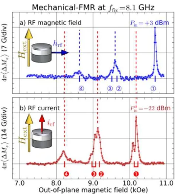
The comparative spectroscopic study performed by mechanical-FMR at ffix= 8.1 GHz on the normally
mag-netized spin-valve nano-pillar is presented in FIG. 2. In these experiments, there is no dc current flowing through the device, and the spectra are obtained in the small ex-citation regime (precession angles less than 5○, see
ap-pendix B 1). The upper panel (a) shows the SW spec-trum excited by a uniform RF magnetic field applied in the plane of the layers, while the lower panel (b) dis-plays the SW spectrum excited by an RF current flowing perpendicularly through the magnetic layers. The strik-ing result is that these two spectra are different: none of the SW modes excited by the homogeneous RF field is present in the spectrum excited by the RF current flow-ing through the nano-pillar, and vice versa.
Let us first focus on FIG. 2a, where the obtained ab-sorption spectrum corresponds to the so-called standard FMR spectrum. Here, the output power of the microwave synthesizer at 8.1 GHz is set to +3 dBm, which corre-sponds to an amplitude of the uniform linearly polarized RF magnetic field hrf≃ 2.1 Oe produced by the antenna
(see appendix B 1). In this standard FMR spectrum, only SW modes with non-vanishing spatial average can couple to the homogeneous RF field excitation. In field-sweep spectroscopy, the lowest energy mode occurs at the largest magnetic field. So, the highest field peak at H➀= 10.69 kOe should be ascribed to the uniform mode.
Since this peak is also the largest of the spectrum, it corresponds to the precession of a large volume in the nano-pillar, i.e., the thick layer must dominate in the
FIG. 2. (Color online) Comparative spectroscopic study
per-formed by mechanical-FMR at ffix= 8.1 GHz, demonstrating
that distinct SW spectra are excited by a uniform in-plane RF magnetic field (a) and by an RF current flowing perpen-dicularly through the layers (b). The positions of the peaks are reported in Table II.
dynamics. In mechanical-FMR, a quantitative measure-ment of the longitudinal magnetization is obtained39,49
(see appendix B 1). The amplitude of the peak at H➀
corresponds to 4π⟨∆Mz⟩ ≃ 14 G, which represents a
pre-cession angle⟨θ⟩ ≃ 3.1○. This sharp peak is followed by a
broader peak with at least two maxima at H➁= 9.65 kOe
and H➂= 9.51 kOe, and at lower field, by a smaller
reso-nance around H➃= 8.64 kOe. Among these other peaks,
there is the uniform mode dominated by the thin layer, which has to be identified and distinguished from higher radial index SW modes.
Let us now turn to FIG. 2b, corresponding to the spec-troscopic response to an RF current of same frequency 8.1 GHz flowing perpendicularly through the nano-pillar. Here, the output power of the microwave synthesizer is −22 dBm, which corresponds to an rms amplitude of the RF current irf ≃ 170 µA (see appendix B 2). The
SW spectrum is acquired under the exact same condi-tions as for standard FMR, i.e., the spherical magnetic probe of the mechanical-FMR detection is kept at the same location above the sample. The striking result is that the position of the peaks in FIGS. 2a and 2b do not coincide. More precisely there seems to be a trans-lational correspondence between the two spectra, which are shifted in field by about 0.5 kOe from each other. The lowest energy mode in the RF current spectrum oc-curs at H➊ = 10.22 kOe. This is again the most intense
peak, suggesting that the thick layer contributes to it, and 4π⟨∆Mz⟩ ≃ 26 G, which represents a precession
an-gle ⟨θ⟩ ≃ 4.2○. This main resonance line is also split in
two peaks, with a smaller resonance in the low field wing of the main peak, about 100 Oe away. At lower field, two distinct peaks appear at H➋ = 9.17 kOe and H➌ =
9.07 kOe and another peak is visible at H➍= 8.22 kOe.
The fact that the two spectra of FIGS. 2a and 2b are distinct implies that they have a different origin. It will be shown in the theoretical section IV A 3 that the RF field and the RF current excitations probe two different azimuthal symmetries ℓ. Namely, only ℓ= 0 modes are excited by the uniform RF magnetic field, whereas only ℓ= +1 modes are excited by the orthoradial RF Oersted field associated to the RF current50. The mutually
exclu-sive nature of the responses to the uniform and orthora-dial symmetry excitations is a property of the preserved axial symmetry, where the azimuthal index ℓ is a good quantum number, i.e., different ℓ-index modes are not mixed and can be excited separately (see section IV A 2).
III. EXPERIMENTAL ANALYSIS
In this section, we first look at the effect of a continuous current flowing through the nano-pillar on the SW spec-tra in order to determine which layer contributes mostly to the resonant signals observed in FIG. 2. Due to the asymmetry of the spin transfer torque in each magnetic layer, the different SW modes are influenced differently depending on the layer in which the precession is the largest. Then, we briefly mention experiments, where spectroscopy is performed by monitoring the dc voltage produced by the magnetization precession in the hybrid nanostructure, and compared to mechanical-FMR. Fi-nally, the analysis of the frequency-field dispersion rela-tion and of the linewidth of the resonance peaks enables to extract the gyromagnetic ratio and the damping pa-rameters in the thick and thin layers.
A. Direct bias current
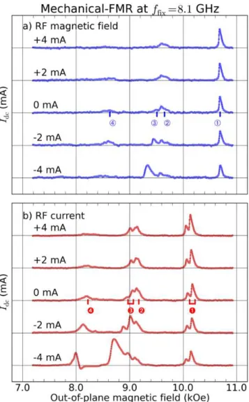
To gain further insight about the peak indexation, we have measured the spectral evolution produced on the SW spectra of FIG. 2 when a finite dc current Idc ≠ 0
is injected in the nano-pillar. We recall that for our sign convention, a positive dc current stabilizes the thin layer and destabilizes the thick one due to the spin trans-fer torque, and vice versa6,7. The results obtained by
mechanical-FMR are reported in FIG. 3.
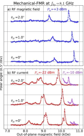
Let us first concentrate on FIG. 3a, in which the ex-citation that probes the different SW modes is the same as in FIG. 2a, i.e., a uniform RF magnetic field. Two main features can be observed in the evolution of the SW spectra as Idc is varied. First, the amplitude of the
peak at H➀ smoothly increases with the positive current
and smoothly decreases with the negative current. At
FIG. 3. (Color online) Evolution of the SW spectra measured
at ffix= 8.1 GHz by mechanical-FMR for different values of
the continuous current Idc flowing through the nano-pillar.
The panel (a) corresponds to excitation by a uniform RF mag-netic field and the panel (b) to excitation by an RF current through the sample.
the same time, the peak at H➂, which is about five times
smaller than the peak at H➀ when Idc = 0 mA, almost
disappears for positive current and strongly increases at negative current, until it becomes larger than the other peaks when Idc= −4 mA. These two features are
consis-tent with the effect of spin transfer if we ascribe the peak at H➀to the uniform mode of mostly the thick layer and
the peak at H➂ to the one of mostly the thin layer. More
precisely, it is expected that in the sub-critical regime (∣Idc∣ < Ith, where Ith is the threshold current for
auto-oscillations, Ith< 0 for the thin layer and Ith> 0 for the
thick layer), the damping scales as α(1−Idc/Ith)25,26(see
appendix A 1), where α is the Gilbert damping parame-ter. It means that the linewidth of a resonance peak that is favored by spin transfer should decrease as the current gets closer to Ith, and that its amplitude, which scales as
the inverse linewidth, should increase.
Although the effect on the peak amplitude noted above is clear in FIG. 3a, it is not on the linewidth. The reason is that in this experiment, the strength of the driving RF magnetic field is kept constant to hrf = 2.1 Oe. As a
re-sult, the shape of the growing peaks in FIG. 3a becomes more asymmetric, which is a signature that the preces-sion amplitude driven by the RF field is strong enough to change the internal field by an amount of the order of the linewidth. This leads to some foldover of the res-onance line51,52, a non-linear effect for which details are
given in the appendix B 1. In other words, the distortion of the line shape as the peak amplitude increases pre-vents to see the diminution of its linewidth53. It would
be necessary to decrease the excitation amplitude as the threshold current is approached26 so as to maintain the
peak amplitude in the linear regime in order to reveal it. The opposite signs of the spin transfer torques which influence the dynamics in the thin and thick layers are thus clearly seen in FIG. 3a. Their relative strengths can also be determined, as the amplitude of the peak at H➂
grows much faster with negative current than the one of the peak at H➀ with positive current. This is because
the efficiency of the spin transfer torque is inversely pro-portional to the thickness of the layer6,7. Whereas the
precession angle in the thick layer does not vary much with Idc (from ≈ 2.5○ at −4 mA to ≈ 3.5○ at +4 mA),
the precession angle that can be deduced from⟨∆Mz⟩ in
the thin layer grows from almost zero at Idc= +4 mA to
more than 6○ at I
dc= −4 mA. Moreover, the peak
posi-tion H➂ shifts clearly towards lower field as the negative
current is increased. This is due to the onset of spin transfer driven auto-oscillations in the thin layer, which occurs at a threshold current Ith≲ −4 mA and produces
this non-linear shift19. We note, that such a value for
the threshold current in the thin layer can be found from Slonczewski’s model (see appendix A 1).
Let us now briefly discuss FIG. 3b, which shows the dependence on Idc of the mechanical-FMR spectra
ex-cited by an RF current excitation. A similar dependence on Idcof the resonance peaks in translational
correspon-dence with FIG. 3a is observed. Again, a clear asymme-try is revealed depending on the polarity of Idc and on
the SW modes. The double peak at H➊ is favored by
positive currents, hence it should be ascribed to mostly the thick layer precessing, while the double peak at H➌
is strongly favored by negative currents, hence it should be ascribed to mostly the thin layer precessing. More-over, a careful inspection shows that the peak H➋, which
looks single at Idc = 0 mA, is actually at least double.
We will explain this splitting of higher harmonics modes in section V B.
To summarize, the passage of a dc current through the nano-pillar enables to determine which layer mostly con-tributes to the observed SW modes, owing to the asym-metry of the spin transfer effect.
B. Voltage-FMR
Our experimental setup also allows to monitor the dc voltage produced across the nano-pillar by the precession of the magnetization in the bi-layer structure. A lock-in detection is used to measure the difference of volt-age across the nano-pillar when the RF is on and off: Vdc= Von− Voff. This can be done simultaneously to the
acquisition of the mechanical-FMR signal, in the exact same conditions (see FIG. 1). Since the presentation of the experimental results requires a specific discussion, the details as well as the graphs will be published elsewhere. Here, we shall only reveal the three main features that can be noticed in the voltage-FMR spectra.
First, even at Idc = 0, dc voltage peaks are
pro-duced across the nano-pillar at the same positions as the mechanical-FMR peaks observed in FIG. 2, with a difference of potential that lies in the 10 nV range for the precession angles excited here. It is ascribed to spin pumping and accumulation in the spin-valve hybrid structure54,55. Second, these voltage resonance peaks
are signed, namely, the SW modes favored at Idc< 0 in
FIG. 3a (for which the thin layer is dominating) produce a positive voltage peak, whereas those favored at Idc> 0
(thick layer dominating) produce a negative voltage peak. This difference between the thick and thin layer contri-butions is ascribed to the asymmetry of the spin accu-mulation in the multi-layer stack56. Third, the relative
amplitudes of the voltage-FMR peaks are different from the mechanical-FMR ones. For instance, the voltage-FMR peak of the thin layer at H➂is slightly larger than
the peak at H➀of the thick layer (and it has an opposite
sign). This illustrates an important difference between the two detection schemes. While mechanical-FMR mea-sures a quantity proportional to the precessing volume, ⟨∆Mz⟩, the voltage-FMR measures an interfacial effect.
Therefore, when the same precession angle is excited in both layers, the voltage-FMR signal associated to each layer is approximately the same, whereas the mechanical-FMR signal from the thin layer is roughly four times smaller than the one from the thick layer, due to their relative thicknesses.
Finally, we mention that voltage-FMR spectroscopy can also record the intrinsic FMR spectrum of the nano-pillar, i.e., in the absence of the spherical MRFM probe above it. This enables to check that the only effect in-troduced by the probe in mechanical-FMR is an overall shift of the SW modes spectra to lower field without any other distortion, and to quantify this shift, found to be −190 Oe57.
C. Gyromagnetic ratio
A precise orientation of the applied magnetic field Hext along the normal ˆz of the sample (polar angle θH = (ˆz,Hext) = 0) enables a direct determination of
the frequency-field dispersion relation of the resonance peaks at H➀ and at H➂ (from 4.5 GHz to 8.1 GHz and
from 6.2 GHz to 11 GHz, respectively) in our nano-pillar, it is found that γ= 1.87 × 10⁷rad.s−1.G−1 is identical in
the thick and thin layers. Moreover, the value of γ mea-sured in the nano-pillar is the same as in the extended reference film (see appendix B 3 and Table I), confirm-ing that the applied field is sufficient to saturate the two magnetic layers and is precisely oriented along ˆz.
The same result is obtained by following the evolu-tion of the frequency-field dispersion relaevolu-tion presented in FIG. 4. Here, we take advantage of the broadband design of the electrodes which connect the nano-pillar to measure the FMR spectrum at fixed bias magnetic field, Hfix = 10 kOe, by sweeping the frequency of the
RF current through it. The data are plotted accord-ing to the frequency scale above FIG. 4a. At con-stant magnetic configuration (above the saturation field, i.e., ≳ 8 kOe), this frequency scale is in correspondence with field-sweep experiments performed at fixed RF fre-quency ffix= 8.1 GHz through the affine transformation
Hext− Hfix= 2π(f − ffix)/γ, as seen from the field scale
below FIG. 4b. This is a direct experimental check of the equivalence between frequency and field sweep ex-periments in the normally saturated state.
D. Damping parameters
From the FMR data presented above, we can also di-rectly extract the damping parameters in each Permalloy layer. Indeed, in field-sweep spectroscopy in the normal orientation (θH = 0), the full width at half-maximum
(FWHM) ∆H of a resonance line is proportional to the excitation frequency ω/(2π) through the Gilbert constant α: ∆H= 2α(ω/γ) (see appendix A 1).
The linewidth of the peak at H➀ associated to mainly
the thick layer in FIG. 2a is equal to ∆H➀ = 48 Oe,
which corresponds to a damping α➀= 0.88 × 10⁻². From
the same mechanical-FMR spectrum, the linewidth of the peak at H➂, associated to mainly the thin layer,
can-not be easily extracted due to the proximity of the peak at H➁. Owing to the interfacial origin of the
voltage-FMR signal, the peak at H➂ is more distinguishable in
the spectrum of the voltage-FMR (not shown), and its linewidth, ∆H➂= 70 Oe, can be fitted. It corresponds to
a damping α➂= 1.29 × 10⁻².
The linewidths of the modes at H➊and H➌can also be
fitted and give similar results for the damping associated to each layer. In the case of the RF current excitation, a frequency-sweep spectrum can be acquired at a fixed bias magnetic field Hfix (see FIG. 4). In that case, the
damping constant is simply obtained by α = ∆f/(2f), where ∆f is the width of the line centered at f . At Hfix = 10 kOe, f➊ = 7.37 GHz and ∆f➊ = 0.12 GHz,
which yield α➊ = 0.81 × 10⁻², and f➌ = 10.92 GHz and
∆f➌= 0.33 GHz, which yield α➌= 1.5 × 10⁻².
In summary, we retain the following values for the
FIG. 4. (Color online) Frequency-field dispersion relation: the
top spectrum (a) is measured at fixed bias field Hfix= 10 kOe
by sweeping the frequency of the RF current irfthrough the
nano-pillar. The bottom spectrum (b) is the same as in
FIG. 2b, and is obtained by sweeping the magnetic field at
fixed frequency ffix = 8.1 GHz of irf. The top and bottom
scales are in correspondence through the affine transforma-tion Hext− Hfix= 2π(f − ffix)/γ.
damping parameters in respectively the thin and the thick layers: αa = (1.4 ± 0.2) × 10−2 and αb = (0.85 ±
0.1) × 10−2. We have reported them, together with γ, in Table I.
These two values are in line with the ones obtained on the reference film, which have also been reported in Ta-ble I. Still, we observe that the linewidths in the nanos-tructure are systematically lower than the ones measured on the reference film. This is a constant characteris-tic that we associate to the confined geometry, which lifts most of the degeneracy (well separated SW modes) and thus strongly reduces the inhomogeneous part of the linewidth observed in the infinite layer15,26. Rather, the
inhomogeneities associated to the magnetic layers15 or
to the confinement geometry will lead to some mode splitting in the nanostructure (see section V B). We have checked that the inhomogeneous contribution to the linewidth in the nano-pillar is weak, by following the de-pendence of the measured ∆H as a function of frequency. In fact, the increase of ∆H➂ from 70 Oe at 8.1 GHz to
105 Oe at 11 GHz is purely homogeneous.
Finally, the finding that the damping is larger in the thin layer than in the thick layer is ascribed to the ad-jacent metallic layers58. In fact, non-local effects such
TABLE I. Magnetic parameters of the thin Pya and thick
Pyb layers measured by cavity-FMR on the reference film
(top row) and by mechanical-FMR in the nano-pillar (bot-tom row). 4πMa(G) αa 4πMb(G) αb γ (rad ⋅ s−1⋅ G−1) 8.2 × 10³ 1.5 × 10⁻² 9.6 × 10³ 0.9 × 10⁻² 1.87 × 10⁷ 8.0 × 10³ 1.4 × 10⁻² 9.6 × 10³ 0.85 × 10⁻² 1.87 × 10⁷
as the spin pumping effect54,59 and the spin diffusion in
the adjacent normal layers by the conduction electrons yield an interfacial increase of the magnetic damping60,
stronger in the case of thin layers.
IV. THEORETICAL ANALYSIS
In this section, we first review a general formalism al-lowing the calculation of the discrete spectrum associ-ated with SW propagation inside a confined body of ar-bitrary magnetic configuration. It is shown that in the two-dimensional (2D) axially symmetric case, different ℓ-index modes can be excited separately, as found ex-perimentally in section II C. The classification of the SW modes in this case is also used to extract the pa-rameters of each magnetic layer from the experimental FMR spectra. In a second part, we discuss the influ-ence of the dynamic coupling between the magnetic disks, where the collective dynamics splits into binding and anti-binding modes. It is shown that in our experimen-tal case, the dynamic dipolar coupling introduces a weak spectral shift, although its influence on the character of the SW modes is real. In the last part, a comparison to full three-dimensional (3D) micromagnetic simulations is performed in order to study in details the collective dy-namics in the nano-pillar.
A. Analytical model
1. General theory
Below, we briefly review the general theory of linear SW excitations (see appendix A 1 for more details). We consider an arbitrary equilibrium magnetic configuration, where the local magnetization writes Msu, with Mˆ s the
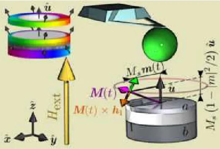
saturation magnetization and ˆuthe unit vector along the local equilibrium direction (implicitly dependent on the spatial coordinates). The linearization of the local equa-tion of moequa-tion is obtained by decomposing the instanta-neous magnetization vector M(t) into a static and dy-namic component61 (see FIG. 5). We shall use the
fol-FIG. 5. (Color online) Schematic representation of the mag-netization dynamics under continuous RF excitation. In the steady state, the torque exerted by the RF perturbation field
h1 (orange arrow) compensates the torque exerted by the
damping (green), and the local magnetization vector M(t)
(purple) precesses at the Larmor frequency on a circular orbit
around the local equilibrium direction (unit vector ˆu). M(t)
is the vector sum of a small oscillating component Msmand
a large static component Ms(1 − ∣m∣2/2), respectively
trans-verse and parallel to ˆu. The inset shows the simulated
spa-tial distribution of ˆuinside the nano-pillar at Hext= 10 kOe
(see section IV C). In the white regions, the magnetization
is aligned along the normal ˆz within 0.05○. In the colored
regions, ˆu is flaring (< 5○) in the radial direction (the hue
indicates the direction of ˆu − ˆz according to the color code
defined in FIG. 6). lowing ansatz: M(t) Ms = ˆu + m(t) + O(m 2), (2)
where the transverse component m(t) is the small dimen-sionless deviation (∣m∣ ≪ 1) of the magnetization from the equilibrium direction. In ferromagnets,∣M∣ = Ms is
a constant of the motion, so that the local orthogonality condition ˆu⋅ m = 0 is required.
Substituting Eq. (2) in the lossless Landau-Lifshitz equation Eq. (A1) (see appendix A 1) and keeping only the terms linear in m, one obtains the following dynam-ical equation for m:
∂m
∂t = ˆu × ̂Ω ∗ m , (3) where here and henceforth, tensor operators are indicated by wide hat, the cross product is denoted by× and the convolution product is denoted by ∗. The self-adjoint tensor operator ̂Ω represents the Larmor frequency:
̂Ω = γH ̂I+ 4πγMsĜ, (4)
where γ is the modulus of the gyromagnetic ratio, H is the scalar effective magnetic field, ̂I is the identity matrix, and ̂G is the linear tensor operator describing
the magnetic self-interactions. The later is the addi-tion of several contribuaddi-tions ̂G(d)+ ̂G(e)+..., respectively the magneto-dipolar interactions, the inhomogeneous ex-change, etc... (see appendix A 2). The effective magnetic field H is a vector aligned along ˆu, whose norm is
H= ˆu ⋅ H0− 4πMsuˆ⋅ ̂G∗ ˆu , (5)
the sum of the ˆu−component of H0, the total applied
magnetic field including the stray field of any nearby magnetic object (in our case, the adjacent magnetic layer in the nano-pillar and the spherical probe), reduced by the static self-interactions, which include the depolariza-tion magnetic field along ˆucreated by the static compo-nent of the magnetization.
SW modes mν are by definition eigen-solutions of
Eq. (3):
−iωνmν= ˆu × ̂Ω ∗ mν. (6)
Here ωνis the SW eigen-frequency and ν is a set of indices
to enumerate the different modes.
The main properties of SW excitations follow from the eigen problem Eq. (6) and the fact that the operator ̂Ω is self-adjoint and real. One can show that the eigen solutions obey the closure relation
i⟨mν⋅ (ˆu × mν′)⟩ = Nνδν,ν′, (7)
where δ is the Kronecker delta function and m stands for the complex conjugate of m. Here we have used the chevron bracket notation introduced in Eq. (1) to denote the spatial average. The quantities Nν are real
normalization constants, which depend on the choice of eigen-functions mν. If the equilibrium magnetization ˆu
corresponds to a (local) minimum of the energy, then the operator ̂Ω is positive-definite. It follows that the “phys-ical” modes with ων > 0 have positive norm Nν > 0. In
this formalism, the eigen-frequencies ωνcan be calculated
as
ων =⟨m
ν⋅ ̂Ω ∗ mν⟩
Nν
. (8)
The importance of this relation is that the frequencies ων calculated using Eq. (8) are variationally stable with
respect to perturbations of the mode profile mν. Thus,
injecting some trial vectors inside Eq. (8) allows one to get approximate values of ων with high accuracy62. The
trial vectors should obey some simple properties: i) they should form a complete basis in the space of vector func-tions m, ii) be locally orthogonal to ˆu and iii) satisfy appropriate boundary conditions at the edges of the mag-netic body63.
2. Normally magnetized disks
In this part, we shall establish a SW modes basis mν
for a normally magnetized disk. A specific feature of the
considered geometry is its azimuthal symmetry. Mathe-matically, this means that the operator ˆu× ̂Ω commutes with the operator ̂Rz that describes an infinitesimal
ro-tation about the ˆzaxis, assuming that the boundary con-ditions are invariant under such a rotation.
This particular configuration allows us to classify the SW modes according to their behavior under the rota-tions in the(x,y) plane. Namely, SW eigen-modes are also eigen-functions of the operator ̂Rzcorresponding to
a certain integer azimuthal number ℓ: ∂m
∂φ − ˆz × m = −i(ℓ − 1)m. (9) Here, φ is the azimuthal angle of the polar coordinate system.
As one can see, Eq. (9) determines the vector struc-ture of SW modes and their dependence on the angle φ. Namely, Eq. (9) for a fixed ℓ has two classes of solutions:
m(1)ℓ = 1 2(ˆx + iˆy)e −iℓφ ψℓ(1)(ρ), (10a) and m(2)ℓ = 1 2(ˆx − iˆy)e −i(ℓ−2)φ ψ(2)ℓ (ρ), (10b) where the functions ψ(1,2)ℓ (ρ) describe the dependence of the SW mode on the radial coordinate ρ and have to be determined from the dynamical equations of motion. So, the azimuthal symmetry allows one to reduce the 2D (ρ and φ) vector equations to a one-dimensional (ρ) scalar problem.
Generally speaking, SW eigen-modes are certain lin-ear combinations of both possible ℓ-forms Eqs. (10). The coupling of these two forms is due solely to the inho-mogeneous dipolar interaction. In our experimental case (lowest energy modes of a relatively thin disk) one can completely neglect this coupling64 and consider only the
right-polarized form Eq. (10a). In the following we will drop the superscript(1) in m(1)ℓ and ψ(1)ℓ .
We shall now find an appropriate set of radial func-tions ψℓ(ρ) to calculate the SW spectrum using Eq. (8).
Here, we can take advantage of the variational stability of Eq. (8) and, instead of the exact radial profiles ψℓ(ρ)
(to find them one has to solve integro-differential equa-tions), use some reasonable set of functions. Namely, it is known that the dipolar interaction in thin disks or prisms does not change qualitatively the profile of SW modes, but introduces effective pinning at the lateral boundaries63. Therefore, we will use radial profiles of the
form ψℓ(ρ) = Jℓ(kℓ,nρ), where Jℓ(x) is the Bessel
func-tion and kℓ,nare SW wave-numbers determined from the
pinning conditions at the disk boundary ρ= R. For our experimental conditions (ta, tb ≪ R), the pinning is
al-most complete, and we shall use kℓ,n = κℓ,n/R, where
κℓ,n is the n-th root of the Bessel function of the ℓ-th
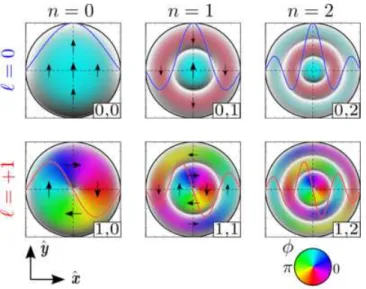
FIG. 6. (Color online) Color representation of the Bessel spa-tial patterns for different values of the azimuthal mode index
ℓ(by row) and radial mode index n (by column). The arrows
are a snapshot of the transverse magnetization mν, labeled
by the index ν= ℓ, n. All arrows are rotating synchronously
in-plane at the SW eigen-frequency. In our coding scheme,
the hue indicates the phase φ = arg(mν) (or direction) of
mν, and the brightness the amplitude of ∣mν∣2. The nodal
positions (∣mν∣ = 0) are marked in white.
FIG. 6 shows a color representation of the Bessel spa-tial patterns for different values of the index ν = ℓ,n. We restrict the number of panels to two values of the azimuthal mode index, ℓ = 0,+1, with the radial index varying between n= 0,1,2. In our color code, the hue indicates the phase (or direction) of the transverse com-ponent mν, while the brightness indicates the amplitude
of ∣mν∣2. The nodal positions are marked in white. A
node is a location where the transverse component van-ishes, i.e., the magnetization vector is aligned along the equilibrium axis. This coding scheme provides a distinct visualization of the phase and amplitude of the preces-sion profiles. The black arrows are a snapshot of the mν
vectors in the disk and are all rotating synchronously in-plane at the SW eigen-frequency.
The top left panel shows the ν = 0,0 (ℓ = 0, n = 0) mode, also called the uniform mode. It usually corre-sponds to the lowest energy mode since all the vectors are pointing in the same direction at all time. Below is the ℓ = +1, n = 0 mode. It corresponds to SWs that are rotating around the disk in the same direction as the Larmor precession. The corresponding phase is in quadrature between two orthogonal positions and this mode has a node at the center of the disk. The variation upon the n = 0,1,2 index (ℓ being fixed) shows higher order modes with an increasing number of nodal rings. Each ring separates regions of opposite phase along the radial direction. All these spatial patterns preserve the rotation invariance symmetry.
FIG. 7. (Color online) Analytically calculated spectra at
Hfix= 10 kOe using the set of Bessel functions (see FIG. 6)
as the trial eigen-vectors. The panel (a) shows the linear re-sponse to a uniform excitation field ˆh1= ˆxand the panel (b)
to an orthoradial excitation field ˆh1 = − sin φ ˆx + cos φ ˆy. A
light (dark) color is used to indicate the energy stored Eq. (12)
in the thin Pya and thick Pyblayers.
3. Selection rules
Using the complete set of Bessel functions in Eq. (8), one can obtain analytically the discrete spectrum of eigen-values for both the thin and thick layers. The de-tails of the numerical application can be found in ap-pendix A 2. The spectral values are displayed in FIG. 7 using vertical ticks labeled ν = jℓn, where j = a,b
indi-cates the precessing layer, and ℓ, n the azimuthal and radial mode indices. They are calculated at fixed applied field Hfix = 10 kOe and placed on the graphs according
to the frequency scale below FIG. 7b, which is in corre-spondence with the field scale above FIG. 7a (see III C for the equivalence between field- and frequency-sweep experiments).
The comparison with the experimental data in FIGS. 2a and 2b shows that the coupling to an exter-nal coherent source depends primarily on the ℓ-index. Indeed, this index carries the discriminating symmetry in SW spectroscopy65. This is because the excitation
ef-ficiency is proportional to the overlap integral hν= ⟨
mν⋅ h1⟩
Nν
, (11)
exci-tation field. It can be easily shown that a uniform RF magnetic field, h1= hrfx, can only excite ℓ= 0 SW modes.
We have shown in FIG. 7a the predicted position of these modes with blue tone ticks. Obviously the largest over-lap is obtained with the so-called uniform mode (n= 0). Higher radial index modes (n≠ 0) still couple to the uni-form excitation but with a strength that decreases as n increases37,66. The ℓ≠ 0 normal modes, however, are
hid-den because they have strictly no overlap with the excita-tion. The comparison with the experimental spectrum in FIG. 2a confirms that conventional FMR67 probes only
partially the possible SW eigen-modes, along the ℓ= 0-index value. In contrast, the RF current-created Oersted field, h1 = hOe(ρ)(−sinφ ˆx + cosφ ˆy) has an orthoradial
symmetry and can only excite ℓ = +1 SW modes. We have shown in FIG. 7b the predicted position of these modes with red tone ticks. They are in good agreement with the resonance positions observed in FIG. 2b. We also note that the ℓ = 0 and ℓ = +1 spectra calculated analytically bear similar a/b and n index series as a func-tion of energy. This explains why the two spectra in FIGS. 2a and 2b look in translational correspondence with each other. We emphasize that the same transla-tional correspondence would have been observed for any higher azimuthal order ℓ> 1 index spectra.
From the coupling to the excitation field expressed by Eq. (11), one can also calculate the mechanical-FMR signal ∝ ⟨∆Mz⟩, proportional to the energy stored in
the magnetic system39,45. For an arbitrary pulsation
fre-quency ω, 4π⟨∆M ⋅ ˆu⟩ ≃ 4πMs∑ ν γ2∣h ν∣2 (ω − ων)2+ Γ2νN ν, (12)
where the SW damping rate Γνis given by Eq. (A8) in
ap-pendix A 1. Eq. (12) is derived under the approximation that the only relevant coefficients in the damping matrix are the diagonal terms. It has been used to compute the relative peak amplitudes in the analytically calculated spectra of FIG. 7.
4. Comparison with experiments
The analytical model outlined in sections IV A 1 and IV A 2 can be used to analyze the experimental spec-tra of FIG. 2, and to exspec-tract some useful parameters of the nano-pillar. More details can be found in the appendix A 2 along with an approximate expression for the SW frequencies in the form of Kittel’s traditional formula (with renormalized values of the effective self-demagnetization fields). This Kittel’s formula, derived for the ℓ = 0 spectrum, should be used to analyze the SW spectrum excited by a uniform RF field to yield the correct values of the magnetization in our nano-pillar. Identifying the experimental peaks at H➂and H➀ as the
lowest energy modes of the thin Pya and thick Pyblayers
yields their respective magnetizations 4πMa= 8.0×10³G
and 4πMb= 9.6×10³G, see Eq. (A32). These values have
been reported in Table I, together with those measured in the reference film (see appendix B 3). The magneti-zations extracted in the nano-pillar are the same as in the extended film. The only small difference concerns the magnetization of the thin layer, which is 200 G lower in the nanostructure than in the reference film (where 4πMa= 8.2 × 10³G). We attribute this to some
interdif-fusion between Py and Cu or Au at the interfaces of the thin layer, which can happen during the etching process of the nano-pillar.
Second, the separation between SW modes crucially depends on the lateral confinement in the nano-pillar and thus on the precise value of its radius. Experimentally, the measured field separation between the two first peaks in FIG. 2a (FIG. 2b), which differ by an additional node in the radial direction, is H➀− H➁ = 1.04 kOe (H➊−
H➋= 1.05 kOe). Using the nominal radius 100 nm in the
analytical model predicts that consecutive n-index mode (n= 0 and n = 1 modes) should be separated by 1.33 kOe, which is larger than the observed value. This separation drops to 1.05 kOe for a larger disk radius R= 125 nm, which we thus refer to as the radius of our nano-pillar. This value of R also allows to estimate the shift between the ℓ= 0 and ℓ = +1 spectra, found to be 530 Oe, in good agreement with the experimental value H➀−H➊= 470 Oe
observed in FIG. 2.
B. Influence of dipolar coupling between different
layers
In the treatment above we have neglected the dynamic coupling between the two magnetic disks in dipolar inter-action. In general, the interaction between two identical magnetic layers will lead to the hybridization of the same ν-index mode of each layer into two collective modes: the acoustic mode, where the layers are precessing in phase, and the optical mode, where they are precessing in anti-phase. This has been observed in interlayer-exchange-coupled thin films68 and in trilayered wires where the
two magnetic stripes are dipolarly coupled69. In the case
where the two magnetic layers are not identical (different geometry or magnetic parameters), this general picture continues to subsist. Although both isolated layers have eigen-modes with different eigen-frequencies, the collec-tive magnetization dynamics still splits in a binding and anti-binding state. But here, the precession of magneti-zation can be more intense in one of the two layers and the spectral shift of the coupled SW modes with respect to the isolated SW modes is reduced, as it was observed in both the dipolarly-69 and exchange-coupled cases70.
Here, we assume that the dominant coupling mecha-nism between the Py layers is the magnetic dipolar inter-action. We neglect any exchange coupling between the magnetic layers mediated through the normal spacer or any coupling associated to pure spin currents14in our
FIG. 8. (Color online) Schematic representation of the cou-pled dynamics between two different magnetic disks. Here,
ωb, the eigen-frequency of the lowest energy precession mode
in the thick layer (the thin layer being fixed at equilibrium)
is smaller than ωa, the one in the thin layer (the thick layer
being fixed at equilibrium). When the two disks are dynam-ically coupled through the dipolar interaction, the binding state B corresponds to the two layers oscillating in anti-phase
at ωB, with the precession occurring mostly in the thick layer,
whereas the anti-binding state A corresponds to the layers os-cillating in phase at ωA, with the precession mostly in the thin
layer. This is shown by displaying the dipolar charges and the
precession profile m(ρ) in each layer using a light (dark) color
to represent the contribution of the thin (thick) layer.
the dipolar coupling between the two magnetic layers, one can complement the perturbation theory derived in the previous section IV A and in the appendix A 1. De-noting cj, the SW amplitudes in j-th disk , one can get
from Eq. (A6): dca
dt = −iωaca+ iγha,bcb, (13a) dcb
dt = −iωbcb+ iγhb,aca, (13b) where ωj is the frequency of the j-th disk (j= a,b) with
account of only the static field of the j′-th disk (j′= b,a)
(i.e., with Mj′ fixed at equilibrium, see FIG. 8). The
cross term hj,j′ is given by
hj,j′= −
4πMj′
Nj ⟨m
j⋅ ̂G(d)∗ mj′⟩
j . (14)
Here, ̂G(d) represents the magneto-dipolar interaction, Mj′ is the saturation magnetization of the j′-th disk and
the averaging goes over the volume of j-th disk. Thus, hj,j′ is the average over the j-th mode of the magnetic
field created by the magnetization of the j′-th disk. It
can be shown that the overlap defined in Eq. (14) is max-imum between mode pairs bearing similar wave-numbers in each layer (i.e., the same set of indices ν)69. This is
the reason why dropping the index ν in Eqs. (13) and (14) is a reasonable approximation.
The anti-binding (A) and binding (B) eigen-frequencies of Eqs. (13) have the form
ωA,B= ωa+ ωb 2 ± √ (ωa− ωb 2 ) 2 + Ω2, (15) where Ω2= γ2ha,bhb,a. (16)
In the case when the dipolar coupling is small (Ω≪ ∣ωa− ωb∣), the eigen-frequencies can be written as (we
assume ωa> ωb) ωA= ωa+ Ω2 ωa− ωb , (17) ωB= ωb− Ω2 ωa− ωb . (18)
These equations can be used for quantitative purposes when Ω/∣ωa− ωb∣ < 0.3 in which case they describe
fre-quency shift with accuracy better than 10%. Thus, the larger of the frequencies (ωa) shifts up by
∆ω= Ω
2
ωa− ωb
, (19)
while the smaller one (ωb) shifts down by the same
amount. This effect is summarized in FIG. 8.
A numerical estimate of the coupling strengths ha,b
and hb,a between the lowest energy SW modes in each
disk can be found in appendix A 2. The obtained re-sult is very close to the approximate estimation used in Ref.71, where the spatial structure of the interacting SW
modes is ignored to calculate the dipolar coupling be-tween uniformly precessing disks. For the experimental parameters, Ω/2π ≃ 0.5 GHz. This coupling is almost an order of magnitude smaller than the frequency splitting ωa−ωb, caused, mainly, by the difference of effective
mag-netizations of two disks: γ4π(Mb− Ma) ≃ 2π ⋅ 4.5 GHz.
As a result, the shift of the resonance frequencies due to the dipolar coupling is negligible, ∆ω/2π ≃ 0.06 GHz.
Using Eqs. (13), one can also estimate the level of mode hybridization due to the dipolar coupling. For instance, at the frequency ωA≈ ωa, the ratio between the
preces-sion amplitudes in the two layers is given by ∣cb/ca∣ωA= ∆ω/(γha,b) ≃
Ω ωa− ωb
. (20) For the experimental parameters, Ω/(ωa− ωb) ≈ 0.1, i.e.,
the precession amplitude in the disk b is about 10 % of that in the disk a. Thus, although the dipolar coupling induces a small spectral shift (second order in the cou-pling parameter, Eq. (19)), its influence in the relative precession amplitude is significant (first order in the cou-pling parameter, Eq. (20)). Finally, we point that here the dipolar coupling is anti-ferromagnetic, and that the binding (lower energy) mode B always corresponds to the thick layer mainly precessing, with the thin layer vi-brating in anti-phase, and vice-versa for the anti-binding (in-phase) mode A (see dipolar charges in FIG. 8).
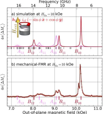
FIG. 9. (Color online) Panel (a) is the numerically calculated
spectral response to a uniform excitation field h1 ∝ ˆx, from
a 3D micromagnetic simulation performed at Hfix= 10 kOe.
The peaks are labeled according to their precession profiles shown in FIG. 11. A light (dark) color is used to indicate the energy stored in the thin (thick) layer. Panel (b) recalls the experimental spectrum measured by mechanical-FMR when exciting the nano-pillar by a homogeneous RF magnetic field at ffix= 8.1 GHz.
C. Micromagnetic simulations
In the analytical formalism presented above, several approximations have been made. For instance, we have assumed total pinning at the disks boundary for the SW modes and no variation of the precession profile along the disks thicknesses (2D model), and we have neglected the dependence on ν of the dynamic dipolar coupling. Still, it allows to extract important parameters in our nano-pillar, such as its radius and the magnetization in both layers. It also describes the influence of the dynamic dipolar coupling on the position and collective character of the SW modes.
Instead of developing a more complex analytical for-malism, we have performed innovative 3D micromagnetic simulations in order to go beyond the approximations mentioned above, and to unambiguously identify the SW modes observed in our nano-pillar sample. For that pur-pose, we have used a combination of micromagnetic sim-ulation solvers available as part of SpinFlow 3D, a finite element based simulation platform for spintronics devel-oped by In Silicio72. The steady state micromagnetic
solver used to obtain numerical approximations of
mi-FIG. 10. (Color online) Panel (a) is the simulated spectral
response to an orthoradial excitation field h1 ∝ − sin φ ˆx +
cos φ ˆy. Panel (b) recalls the experimental spectrum measured
by mechanical-FMR for an RF current excitation.
cromagnetic equilibrium states is based on a weak for-mulation and Galerkin type finite element implementa-tion of the very efficient projecimplementa-tion scheme introduced in Ref.73. A second numerical solver, a micromagnetic
Eigen solver, has been used for fast calculations of loss-less 3D SW eigen-modes. It is based on a finite element discretization of the generalized eigen-value problem de-fined by the linearized lossless magnetization dynamics in the vicinity of an arbitrary pre-computed equilibrium state, following an approach very similar to the one in-troduced in Ref.74. The discrete generalized eigen-value
problem is solved with an iterative Arnoldi method us-ing the ARPACK library75. In this calculation the full
complexity of the 3D micromagnetic dynamics of the presently considered bilayer system is preserved. The solver outputs both the eigvalues by increasing en-ergy order and the associated eigen-vectors. Several tens of SW eigen-modes can be accurately computed in a mat-ter of few minutes of CPU time with a standard desktop PC, for magnetic thin film nano-structures with typi-cal lateral sizes in the 100 nm range. This is two to three orders of magnitude faster compared to the re-quired computation time when using more traditional approaches for micromagnetic computation of SW eigen-modes, which are typically based on the Fourier com-ponent analysis of time series generated by the solution of the full non-linear Landau-Lifshitz-Gilbert equation76.
implement-ing among other thimplement-ings the spectral decomposition of the MRFM signal as expressed in Eqs. (11), (12) and (A8), has been used to compute the MRFM spectra shown here.
To proceed, the nano-pillar is first discretized using unstructured meshing algorithms resulting in an aver-age mesh size of 3.5 nm. This corresponds to a total number of vertices in the vicinity of 5× 10⁴. The
mag-netization vector is interpolated linearly inside each cell (tetrahedra) – a valid approximation taking into account that the cell sizes are smaller than the exchange length Λex ≃ 5 nm in Permalloy. The magnetic parameters
in-troduced in the code are the ones reported in Table I, and the simulation incorporates the perturbing presence of the magnetic sphere attached on the cantilever. More-over, the 10 nm thick Cu spacer is replaced by vacuum, so that the layers are only coupled through the dipolar interaction (spin diffusion effects are absent).
The next step is to calculate the equilibrium config-uration in the nano-pillar at Hext = Hfix = 10 kOe.
The external magnetic field is applied exactly along ˆz and the spherical probe with a magnetic moment m = 2× 10⁻¹⁰emu is placed on the axial symmetry axis at a
distance s= 1.3 µm above the upper surface of the nano-pillar. The convergence criterion introduced in the code is ∣dMz/Mj∣ < 2 ⋅ 10−9 between iterations. The result
shown in the inset of FIG. 5 reveals that the equilib-rium configuration is almost uniformly saturated along
ˆ
z. Still, a small tilt (< 5○) of the magnetization, away
from ˆz and along the radial direction, is observed at the periphery of the thick and thin layers.
The micromagnetic eigen solver is then used to com-pute the lowest eigen-values of the problem as well as the associated eigen-vectors. The discrete list of eigen-values under 18 GHz is shown as black vertical ticks at the bot-tom of FIGS. 9a and 10a. The precession patterns of the six vectors corresponding to the six lowest eigen-frequencies are shown in FIG. 11. The middle and right columns show the dynamics m in the thin Pya and thick
Pyblayers, while the precession profiles along the median
direction are shown on the left in light and dark colors, respectively. The resonance peaks are labeled according to the SW modes precession profiles and the eigen-values of the simulated peaks are reported in Table II.
From the eigen-vectors spatial patterns, one can com-pute their coupling (Eq. (11)) to a uniform RF field h1=
hrfxˆ and, with Eq. (12), the mechanical-FMR spectrum
(FIG. 9a). The same procedure is repeated for the RF current-induced Oersted field h1∝ irf(−sinφ ˆx + cos φ ˆy)
excitation (FIG. 10a). Since the code gives access to the contribution of each layer, a light (dark) tone is used to indicate the vibration amplitude in the thin (thick) layer in the two figures. For comparison, the mechanical-FMR spectra of FIGS. 2a and 4a have been reported in FIGS. 9b and 10b, respectively. We have applied the same conversion between the frequency (top) and field (bottom) scales as discussed in section III C.
In FIG. 9a, the largest peak in the simulation occurs at
TABLE II. Comparative table of the resonance values for the SW modes, arranged in order of increasing energy. On the left are the consecutive peak locations measured experimentally.
Experiments are performed at ffix = 8.1 GHz (FIG. 2) or
Hfix = 10 kOe (FIG. 4a). On the right are the simulated
eigen-frequencies f at Hfix= 10 kOe. The conversion to field
value Hextis obtained through Hext− Hfix= 2π(f − ffix)/γ.
Exp. f (GHz) Hext(kOe) Simu. f (GHz) Hext(kOe)
➀ 10.69 B00 6.08 10.68 ➊ 7.37 10.22 B10 7.44 10.22 ➁ 9.65 B01 8.95 9.71 ➂ 9.51 A00 9.82 9.42 ➋ 10.48 9.17 B11 10.47 9.20 ➌ 10.92 9.07 A10 10.85 9.08 ➃ 8.64 A01 11.98 8.69 ➍ 13.41 8.22 A11 13.19 8.29
the same field as the experimental peak at H➀. This
low-est energy mode corresponds to the most uniform mode with the largest wave-vector and no node along the ra-dial direction, thus it has the index n= 0. It has uniform phase along the azimuthal direction, which is the char-acter of the ℓ= 0 index. For this mode, the thick layer is mainly precessing, with the thin layer oscillating in anti-phase (binding index B), as can be seen from its spatial profile in FIG. 11. The same analysis can be made for the second peak, labeled B01, which occurs close to the
peak at H➁. It also corresponds to a resonance mainly
of the thick layer, and its color representation shows that this is the first radial harmonic (n= 1), with one line of nodes in the radial direction. Again, the thin layer is os-cillating in anti-phase, with the same radial index n= 1, as clearly shown by the mode profile along the median direction. The third peak is labeled A00 and is located
close to the experimental peak at H➂. It corresponds this
time to a uniform (n= 0) precession mainly located in the thin layer, in agreement with the experimental analysis presented in section III A. In this mode, the thick layer is also vibrating in phase with the thin layer (anti-binding index A).
We can also look at the relative amplitudes of preces-sion in the two disks to quantify the dynamic coupling between the disks. From the profiles shown in FIG. 11, one can infer that for the fundamental mode B00, the
am-plitude of precession is distributed with a ratio of about 3:1 between the thick (75%) and the thin layer (25%). For the mode A00, the ratio is 8:1 in favor of the thin
layer, which contributes to 89% of the precession ampli-tude (11% for the thick layer). These relative preces-sion amplitudes were expected from the relative weight of the thick and thin layers and from the approximate analytical model presented in section IV B. The simu-lated field separation between the two coupled uniform modes (ωB00 − ωA00)/γ = 1.28 kOe compares also well
with the 1.30 kOe estimate from the 2D model, with the dynamic dipolar coupling taken into account. Finally, one can check from the simulations the independence of