Publisher’s version / Version de l'éditeur:
Vous avez des questions? Nous pouvons vous aider. Pour communiquer directement avec un auteur, consultez la première page de la revue dans laquelle son article a été publié afin de trouver ses coordonnées. Si vous n’arrivez pas à les repérer, communiquez avec nous à [email protected].
Questions? Contact the NRC Publications Archive team at
[email protected]. If you wish to email the authors directly, please see the first page of the publication for their contact information.
https://publications-cnrc.canada.ca/fra/droits
L’accès à ce site Web et l’utilisation de son contenu sont assujettis aux conditions présentées dans le site LISEZ CES CONDITIONS ATTENTIVEMENT AVANT D’UTILISER CE SITE WEB.
The Journal of Chemical Physics, 128
READ THESE TERMS AND CONDITIONS CAREFULLY BEFORE USING THIS WEBSITE. https://nrc-publications.canada.ca/eng/copyright
NRC Publications Archive Record / Notice des Archives des publications du CNRC :
https://nrc-publications.canada.ca/eng/view/object/?id=0fe78fea-ca86-40e8-b36e-af39312a8615
https://publications-cnrc.canada.ca/fra/voir/objet/?id=0fe78fea-ca86-40e8-b36e-af39312a8615
NRC Publications Archive
Archives des publications du CNRC
This publication could be one of several versions: author’s original, accepted manuscript or the publisher’s version. / La version de cette publication peut être l’une des suivantes : la version prépublication de l’auteur, la version acceptée du manuscrit ou la version de l’éditeur.
For the publisher’s version, please access the DOI link below./ Pour consulter la version de l’éditeur, utilisez le lien DOI ci-dessous.
https://doi.org/10.1063/1.2932101
Access and use of this website and the material on it are subject to the Terms and Conditions set forth at
Time- and frequency-resolved coherent anti-Stokes Raman scattering
spectroscopy with sub-25 fs laser pulses
Lausten, Rune; Smirnova, Olga; Sussman, Benjamin J.; Gräfe, Stefanie;
Mouritzen, Anders S.; Stolow, Albert
Time- and frequency-resolved coherent anti-Stokes Raman scattering
spectroscopy with sub-25 fs laser pulses
Rune Lausten,1,2,a兲Olga Smirnova,2Benjamin J. Sussman,1Stefanie Gräfe,2 Anders S. Mouritzen,3and Albert Stolow1,2
1
Department of Physics, Queen’s University, Kingston, Ontario K7L 3N6, Canada
2
Steacie Institute for Molecular Sciences, National Research Council of Canada, Ottawa, Ontario K1A 0R6, Canada
3
Department of Physics and Astronomy, University of Aarhus, DK-8000 Århus C, Denmark
共Received 14 February 2008; accepted 29 April 2008; published online 26 June 2008兲
In general, many different diagrams can contribute to the signal measured in broadband four-wave mixing experiments. Care must therefore be taken when designing an experiment to be sensitive to only the desired diagram by taking advantage of phase matching, pulse timing, sequence, and the wavelengths employed. We use sub-25 fs pulses to create and monitor vibrational wavepackets in gaseous iodine, bromine, and iodine bromide through time- and frequency-resolved femtosecond coherent anti-Stokes Raman scattering共CARS兲 spectroscopy. We experimentally illustrate this using iodine, where the broad bandwidths of our pulses, and Boltzmann population in the lower three vibrational levels conspire to make a single diagram dominant in one spectral region of the signal spectrum. In another spectral region, however, the signal is the sum of two almost equally contributing diagrams, making it difficult to directly extract information about the molecular dynamics. We derive simple analytical expressions for the time- and frequency-resolved CARS signal to study the interplay of different diagrams. Expressions are given for all five diagrams which can contribute to the CARS signal in our case. © 2008 American Institute of Physics.
关DOI:10.1063/1.2932101兴
I. INTRODUCTION
There is considerable effort devoted to the generation of increasingly shorter pulses of visible light. The development of ultrashort pulse Ti:sapphire oscillators has led to near-infrared 共NIR兲 pulses shorter than 7 fs at 800 nm 共Refs. 1
and 2兲 and tunable visible pulses as short as 29 fs from 400 nm synchronously pumped optical parametric oscillators.3 For amplified laser pulses, the development of the noncollinear optical parametric amplifier4 共NOPA兲 has produced pulses in the visible and NIR region as short as 5 fs.5These, in combination with broadband phase matching schemes for second harmonic generation, have resulted in UV pulses below 10 fs in duration.6One of the most impor-tant applications of this technology is to problems in con-densed phase molecular dynamics where ultrafast electronic dephasing times often obscure the spectroscopic and dynami-cal information being sought. In order to address these is-sues, various nonlinear optical 共NLO兲 spectroscopies have been developed7 which help disentangle the various contri-butions of the material response to applied optical laser fields. Due to the inversion symmetry of molecules in bulk noncrystalline media, the lowest order NLO response of gen-eral utility is at third order, of which coherent anti-Stokes Raman scattering 共CARS兲 is a well known example. When combined with ultrashort laser pulses, CARS can reveal de-tailed dynamics within excited molecules in both gas8,9 and condensed phases. The CARS process involves the
interac-tion of three laser fields, generating a third order polarizainterac-tion whose associated emitted field is measured in a phase-matched direction. As discussed by Faeder et al.,10 the ex-pression for the third order polarization includes all possible time orderings of the three interactions. The spectroscopic pathways producing the third order polarization may be de-picted using double-sided Feynman diagrams, as shown, for example, in Fig. 3 of Ref.10.
In this paper we consider the case where a pump and Stokes pulse always overlap and only five of the eight dif-ferent diagrams given in Ref. 10can contribute to the fem-tosecond time-resolved CARS signal, depending on the de-lays. Defining the pump/Stokes pulse pair overlap as t = 0, the situation where the delayed pump pulse arrives before 共after兲 t=0 thus corresponds to negative 共positive兲 delays. These diagrams and their labels are reproduced from Ref.11
in Fig. 1.
For “cold” molecules we need only consider diagram A for ⌬t ⬍ 0 and diagram C for ⌬t ⬎ 0, since diagrams B, D, and E all require excited vibrational states to be populated, e.g., via the Boltzmann distribution at a finite temperature.
For the case of “hot” molecules, it is sometimes possible to suppress contributions from the unwanted diagrams. More generally, however, all contributions must be considered and the detected signal is the coherent sum of the fields due to each diagram. These fields, for the case of homodyne detec-tion, are then squared on the detector, leading to various cross terms and interferences.
In the present paper we focus on the femtosecond time-resolved CARS signal for negative time delays. The
selec-a兲Electronic mail: [email protected].
0021-9606/2008/128共24兲/244310/13/$23.00 128, 244310-1 © 2008 American Institute of Physics
tion mechanisms which apply to hot molecules have been discussed by Faeder et al.:10 There are two complementary factors which can lead to suppression of diagram B. First, if the detuning between the Stokes and pump pulses, 共Ev− E0 =p−S兲, is large compared with the vibrational level spac-ing and kBT, diagram B will be suppressed since there will be
no population in the vibrationally excited state, Ev, from which the Stokes photon can be absorbed. Second, the pump wavelength is usually chosen close to the maximum of the electronic absorption band, and the Stokes shift chosen large enough for the Stokes pulse to be away from this resonance. Consequently, even if the vibrational levels Ev required for the first condition are populated, the absorption cross section for the Stokes pulse can be small, favoring energy level dia-gram A over diadia-gram B.
Important to the present paper is the fact that these cri-teria become difficult to fulfill when ultrashort pulses are used: the inherently very broad bandwidths of sub-25 fs pulses can lead to Stokes shifts that are still within spectral overlap of the pulses involved. If neither of the above criteria are met, then both diagram contribute to the third order sig-nal propagating in the phase-matched direction.
Ultrashort pulse CARS spectroscopy of complex samples requires more careful consideration of the various interactions in order to properly describe the observed sig-nals. Unfortunately, the complexity of some systems and/or environments may make assessment of these criteria quite challenging. Our goals here are to 共i兲 clearly illustrate the case for ultrashort pulse CARS spectroscopy when both pro-cesses shown in Fig.1are involved and共ii兲 discuss how one
can treat the interfering contributions to the measured signal. In the following, we use both experimental results from sub-25 fs CARS spectroscopy and a simple analytical model describing the CARS process. We have chosen the well known gas phase system molecular iodine I2, which was heated to 360 K in order to increase its vapor pressure. At these temperatures, three to four vibrational levels are popu-lated within the ground electronic state, and the contribution from each of these states has to be considered separately.
Iodine I2 was one of the first systems to be systemati-cally studied using femtosecond pump-probe spectroscopy in the gas phase.12,13Iodine has long served as a model system in the development of new femtosecond techniques such as time-resolved photoelectron spectroscopy,14 time-resolved Coulomb explosion,15 and femtosecond coherent nonlinear spectroscopies.8,16The dynamics of I2was also used to study the femtosecond spectroscopy of complex environments such as rare gas collisional systems,17 cryogenic matrices,18 and zeolites.19Relevant to the present effort, detailed studies by Knopp et al.20 demonstrated the virtues of using I2 as a model system for studies in femtosecond coherent nonlinear spectroscopy and control.
In the following, we present our combined experimental-theoretical studies of femtosecond time- and frequency-resolved CARS spectroscopy of gas phase iodine共I2兲,
21
bro-mine共Br2兲, and iodine bromide 共IBr兲. In order to address the issues discussed above, we used 艋25 fs duration pulses and heated samples ensuring a broad Boltzmann distribution of rotational and vibrational states. We spectrally dispersed the signals scattered into the phase-matched direction, revealing both details of the wavepacket dynamics and the interfering contributions from the involved diagrams. Under isolated conditions, the induced coherence can persist for extremely long times, leading to the observation of wavepacket revivals22and fractional revivals.23–27The revivals and frac-tional revivals of vibrafrac-tional wavepackets in diatomic mol-ecules were studied experimentally for a number of systems, including the molecules of interest here, iodine,12–14,28 bromine,29,30and iodine bromide.31,32
Finally, as described in the Appendix, we outline a simple analytical model for calculating the third order polar-izations based on the pole approximation, permitting a clear view of the contributions from the different diagrams. Our results illustrate how time- and frequency-resolved four-wave mixing with ultrashort pulses can lead to the observa-tion of regular or apparently irregular wavepacket dynamics, depending on which observation window is chosen for the spectrally resolved scattered signal. In ultrashort pulse coher-ent nonlinear spectroscopies of complex systems/ environments, we expect that unambiguous extraction of the underlying molecular dynamics from these observables will generally require considerations of the type discussed here.
II. TIME-RESOLVED FREQUENCY INTEGRATED CARS SIGNAL
In a well designed third order experiment, one would prefer the polarization to be dominated by a single diagram. This arguably yields the most transparent view of the
under-FIG. 1. Energy level diagrams, illustrating the vibrationally resonant inter-actions contributing to the femtosecond time-resolved CARS signal for negative and positive delays between the pump/Stokes pulse pair at t = 0 and the delayed pump pulse. The interactions with the pump共p兲 pulse and the pump共p兲/Stokes 共S兲 pulse pair are sketched. When very short pulses are used共e.g., sub-25 fs兲, the scattered signals arising from these interactions may be spectroscopically overlapping, leading to polarization beats which dramatically affect the form of the pump-probe signals. In complex samples or environments, it may not be possible to ensure that only one interaction dominates, especially when ultrashort pulses are applied共Ref. 7兲. These diagrams are reproduced from Ref. 11. The corresponding Feynman dia-grams can be seen in Ref.10.
lying molecular dynamics which modulates the observed sig-nals. Central to this paper, however, is the fact that this “single diagram” picture will fail for as simple a sample as gas phase I2 at 360 K, probed by sub-25 fs laser pulses. In order to understand the consequences, we begin by consid-ering the contribution to the CARS signal at t ⬍ 0 from the single diagram labeled A in Fig.1. For a homodyne detection scheme, the transient CARS signal is calculated by time in-tegrating the third order polarization P共3兲as
S共⌬t兲 =
冕
−⬁⬁
dt兩P共3兲共t,⌬t兲兩2
. 共1兲
Here t is the time and ⌬t denotes the positive temporal sepa-ration between the single pump pulse and the Stokes/pump pulse pair. The polarization is given as
P共3兲共t,⌬t兲 =
兺
n=0 3
具共3−n兲共t,⌬t兲兩ˆ兩共n兲共t,⌬t兲典, 共2兲 where ˆ is the dipole operator 关after averaging over elec-tronic degrees of freedom,ˆ共R兲 connecting the ground and
excited electronic state is replaced with a constant in the Condon approximation兴. The brackets denote integration over the bondlength R and the wave functions determined within j
⬘
th order perturbation theory are denoted as共j兲.The CARS signal, originating from the matrix element
a03:
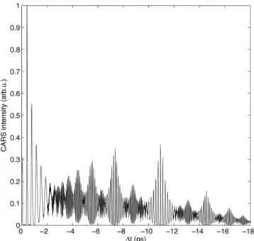
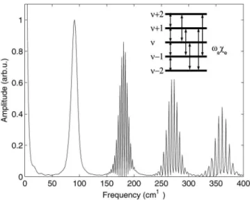
a03共t,⌬t兲 = 具共0兲共R,t兲兩ˆ兩共3兲共R,t,⌬t兲典, 共3兲 oscillates as a function of time delay ⌬t, and contains beat frequencies corresponding to energy level spacings in the electronically excited state. Therefore, the time-resolved CARS signal is a direct reflection of the vibrational wave-packet motion in the excited state, the dynamics of which is well known.29,30An example of an excited state CARS tran-sient calculated by numerical wavepacket propagation, using techniques similar to those used by Meyer et al.33 共with pa-rameters pertaining to our experiment兲, can be seen in Fig.2. In these calculations we include only the vibrational degree of freedom, since the role of the many rotational levels has been investigated previously.34 The fast Fourier transform 共FFT兲 of this transient is shown in Fig.3.
The fundamental peak in the FFT shows coherences be-tween nearest-neighbor vibrational levels and is centered on the average vibrational frequency of the wavepacket 共兲. When resolved in the FFT,29,30each peak corresponds to the vibrational energy level splitting between and its nearest-neighbor + 1. The peaks at this fundamental frequency are separated by the vibrational anharmonicity termee. In the present case, however, we do not resolve the individual peaks in the fundamental frequency region due to the calcu-lation being truncated before the full revival. At the second harmonic frequency, another peak centered at 共2兲 can be seen, corresponding to coherences between next nearest neighbors, and + 2. The splitting between peaks in this case29,30is thus 2ee. The still higher order coherences are to be understood in an analogous manner. These results illus-trate how, when a single CARS diagram is involved, the measured signal transparently reflects details of the excited
state vibrational wavepacket dynamics. As we discuss in the following, when the single diagram picture fails 共our case兲, the observed signals do not so transparently reflect the mo-lecular dynamics and both time-resolved and frequency-resolved measurements are required to disentangle the con-tributions of different diagrams.
III. EXPERIMENTAL
For our experiments, we constructed a dispersion-free, polarization maintaining time- and frequency-resolved CARS spectrometer. Several groups have previously shown how time resolving the electronically resonant CARS
pro-FIG. 2. 共Color online兲 Pulse and level scheme for the time-resolved CARS experiments on “cold” molecules, illustrating how either excited state or ground state dynamics can be studied, depending on the delay. For ⌬t ⬍ 0 via diagram A, for ⌬t ⬎ 0 through diagram C of Fig. 1. The third order process involves a pump pulse共p兲 delayed with respect to the Stokes/pump
pulse pair共S/p兲. These three fields generate a third order polarizability in
the molecules, leading to emission of the CARS signal at the anti-Stokes frequency 共AS兲. All polarizations are parallel, as shown in the lower
diagram.
FIG. 3. Calculated CARS signal for wavepacket dynamics in the I2B-state,
using the method described in Sec. II. The parameters were chosen so as to correspond to our experimental conditions.
cess can be used to study both ground and excited state dy-namics in I2 by detection at a particular wavelength,
16,35
or by dispersed broadband detection.8,36 We therefore summa-rize only briefly. Defining the overlap of pump/Stokes pulses to be t = 0, we introduce a delay ⌬t of the second pump interaction with respect to this. If we now tune the wave-lengths of the pump/Stokes pulses responsible for the CARS process into the B共3⌸
0u
+兲←X共1⌺ 0g
+兲 electronic resonance, the CARS signal will probe either the dynamics of the ground or excited state depending on the delay between the single pump pulse, and the pump/Stokes pulse pair. For negative delays, the single pump pulse arrives first, creating a vibra-tional wavepacket in the excited state, which can then later be probed by the Stokes/pump pulse pair. For positive de-lays, the pump/Stokes pulse pair creates a vibrational wave-packet in the ground electronic state, the dynamics of which can be followed by scanning the delay of the last pump pulse completing the CARS process共see Fig.4兲. Specifically using parameters relevant to the experiment, we start from the ground state, at thermal equilibrium at 360 K, with a 25 fs pump pulse centered at 540 nm. This creates a vibrational wavepacket in the B-state of iodine centered at v
⬘
= 28 and spanning nine to ten vibrational levels. The wavepacket un-dergoes field-free evolution and is subsequently probed through interaction with the 25 fs Stokes pulse centered at 565 nm and the second pump pulse, thus completing the CARS sequence. By spectrally dispersing the anti-Stokes signal, we discern the time- and frequency-resolved wave-packetdynamics.
A block diagram of the experimental arrangement is given in Fig. 5. The samples iodine, bromine, or 共purified兲 iodine bromide were introduced into a heatable closed quartz cell with thin 共1 mm兲 fused silica windows.
The three ultrashort optical pulses required for the CARS experiment are derived from a Ti:sapphire oscillator and 1 kHz regenerative amplifier system, as shown in Fig.5. Approximately 500J/pulse共80 fs at 800 nm兲 of the
ampli-fied light is used to pump two NOPAs, resulting in widely tunable sub-20 fs pulses with pulse energies of⬃10J. One of the NOPA pulses, acting as the pump in the CARS pro-cess, was split by a 1 mm thick inconel coated quartz beam-splitter. The three CARS pulses were delayed appropriately with computer controlled stages, and overlapped in the non-collinear folded-BOXCARS beam geometry. This ensures that the CARS signal propagates in a direction different from the three input beams and can therefore be collected background-free. In addition, it also rules out contributions from other third order processes which do not phase match in this same direction.
Due to the problems with the dispersion management of sub-20 fs pulses, we employed a Cassegrain-based geometry for focusing共inset in Fig.5兲. This has the advantage, due to its all-reflective design, of being both achromatic and dispersion-free. In addition, due to the small angles共⬃1.8°兲 of incidence, this geometry minimizes any polarization rota-tion due to reflecrota-tion from metal surfaces and therefore is polarization maintaining. Finally, we note that this geometry is ideal for bringing a fourth beam along the centerline of the
FIG. 4. The Fourier transform of the CARS signal from Fig.3. The inset shows how coherences between different vibrational levels of the wave-packet give rise to the peaks in the Fourier transform. Details are discussed in the text.
FIG. 5. Dispersion-free, polarization maintaining time- and frequency-resolved CARS spectrometer. A regenerative Ti:sapphire amplifier produces 80 fs pulses pumping two NOPAs, each yielding tunable sub-20 fs optical pulses. Three optical delay lines control their relative timing. The beams are arranged in the folded-BOXCARS configuration and focused using an all-reflective Cassegrain setup, which is dispersion-free and polarization main-taining. Details of this setup are shown in insets A–C. The CARS process generates a third order response at the common focus and leads to emission of anti-Stokes radiation in the phase-matched direction. The CARS signal is dispersed in an imaging spectrometer, where its full spectrum can be col-lected at each time delay.
Cassegrain, allowing for pump-FWM experiments, where the three-pulse FWM scheme can be used to study multiple timescale dynamics induced by a fourth pump pulse.37
The CARS signal was spatially separated from the Stokes and pump beams by an iris, collimated with a lens and propagated a long path length 共⬃20 m兲 in order to re-move residual scattered light background. It was then spec-trally dispersed in an f = 300 mm imaging spectrometer 共Ac-ton SP300i兲 and detected by a 1024⫻252 pixel cooled charge coupled device 共CCD兲 array detector. An electronic shutter built into the spectrometer controlled the average light exposure. Typically 500–1000 pulses were averaged on the CCD chip per time delay step. The quartz sample cell was heated, for iodine, to a temperature of 360 K, corre-sponding to a vapor pressure of 35 Torr. For bromine and iodine bromide, the sample cell was at room temperature 共due to their higher vapor pressures兲.
IV. RESULTS AND DISCUSSION
In Fig. 6 we present the time- and frequency-resolved CARS spectrum for iodine. As discussed in Sec. III, the ⬃25 fs pump and Stokes pulses were chosen to be electroni-cally resonant with the B ← X transition. The time delay was scanned ⫾10 ps in steps of 25 fs. It can be seen that, due to the ultrashort input pulses, the spectrum of the scattered third order signal is very broad—about 50 nm wide. For the input wavelengths used in this experiment, we would expect to find the anti-Stokes signal centered at AS= 2P−S = 19 181 cm−1 共519 nm兲. The data show clear evidence of two regions, at negative and positive time delays, exhibiting different behavior.
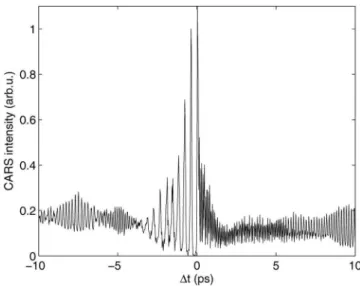
As an illustrative example, we take a cut along the line at AS= 520 nm, shown in Fig. 7, where the center of the anti-Stokes spectrum is expected. The well known B-state wave-packet dynamics is seen at negative time delays whereas
X-state dynamics is seen at positive time delays. In Fig.8we show the FFT power spectra of the data from Fig.7. Again, these power spectra show that the ⌬t ⬍ 0 and ⌬t ⬎ 0 regions correspond to the observation of vibrational wavepacket dy-namics in either excited B-state or ground state X-state, re-spectively.
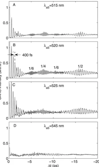
We concentrate herein on excited state wavepacket dy-namics, corresponding to negative time delays where the pump pulse creates a wavepacket in the excited B-state which is then probed as a function of the delay ⌬t of the Stokes/pump pulse pair. We take four illustrative cuts of the two-dimensional共2D兲 data in Fig.6 at AS= 515, 520, 525, and 545 nm. These are shown in Figs. 9共a兲–9共d兲, respec-tively. The 共A兲–共C兲 plots show quite similar behavior: a strong oscillation with an average period of 400 fs from 0 to 4 ps, which revives at 17 ps and again 34 ps 共not shown兲, corresponding to vibrational wavepacket dynamics in the excited B-state. Due to the anharmonicity of the po-tential, the wavepacket spreads共or dephases兲 but undergoes a series of rephasings and partial rephasings, leading to re-vival and fractional rere-vival structures.23,29The initially pre-pared wavepacket is recreated at the full revival at 34 ps共not shown兲. The initial wavepacket can also reform on the outer turning point of the potential, called a half revival,23,29 as observed at 17 ps. An interesting behavior is observed in the intermediate region, where the wavepacket goes through various fractional revivals. For example, at the quarter re-vival, the wavepacket is split into two equal parts exactly out of phase, leading to the doubling of the modulation fre-quency as clearly seen in the data. At the one-sixth revival, the wavepacket is split into three equal parts, leading to a tripling of the modulation frequency, and so on.23,29Note that the magnitude of the revivals is significantly lower than that of the initial wavepacket oscillation 共first 4 ps兲 due to the decay of the rotational anisotropy that was created by the first pump pulse. If desired, this can be avoided by using magic angle detection, as previously described.9
FIG. 6.共Color兲 Time- and frequency-resolved femtosecond CARS spectrum of iodine. The ordinate is the time delay between single pump and the Stokes/pump pulse pair. This 2D data set contains a wealth of information about both excited and ground state dynamics, most clearly illustrated by taking cuts at particular wavelengths AS. Aside from canonical wavepacket
dynamics, the data also reveal interesting beating patterns related to the interference between different contributions to the third order polarization. For a detailed discussion, see the text.
FIG. 7. A cut through the CARS data at AS= 520 nm from Fig.6. For
negative time delays, excited state dynamics is observed, ground state dy-namics for positive delays. Based on the center wavelengths of the pump and Stokes pulses, this cut corresponds to where the CARS signal is ex-pected to be strongest.
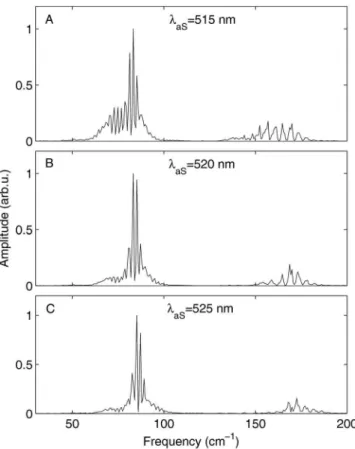
As shown in Fig.10, Fourier transform power spectra of the data in Figs.9共a兲–9共c兲confirm that the oscillations in the transients result from a coherent superposition of vibrational eigenstates with energy spacings centered around 83 cm−1. This corresponds to the spacing between two neighboring vibrational eigenstates in the anharmonic region of the
B-state in iodine at v
⬘
= 28, the levels accessed by the pump pulse at 540 nm. Comparing the FFT power spectra of the three different anti-Stokes wavelengths 515, 520, and 525 nm, we also see that the peak center moves toward lower wavenumbers, as the detection wavelength is shifted toward the blue. As expected, selecting different parts of the scattered CARS spectrum corresponds to monitoring the dy-namics of different parts of the wavepacket.An important point is the distinction between how many vibrational levels the prepared wavepacket spans on one hand versus how well the experimental technique probes these levels. Using a certain technique, we might only be able to observe coherences between a specific subset of the levels that we prepare. We are mainly limited by the Frank–
Condon factors for the probe step, which will depend on the wavelengths chosen for the experiment. In our case, where the pump and Stokes pulse spectra partially overlap, the small detuning of these wavelengths is the key to our obser-vation of higher order revivals in the wavepacket signal, since this ensures effective probing of all the levels in the prepared state. With the time- and frequency-resolved data presented, we are thus able to follow the nuclear dynamics over a significant fraction of its periodic trajectory.
An elegant way of representing the wavepacket evolu-tion is to use a sliding window Fourier transform or spectrogram.38In this method, the product of the time delay scan, S共t兲, and a Gaussian window function, g共t兲 = exp共−t2/t
0 2
兲 and width t0共chosen here to be 0.75 ps兲 is Fou-rier transformed. The spectrogram signal is thus given by
S共, ⌬t兲=兰0
⬁S共t兲g共t−⌬t兲exp共−it兲dt. By translating the win-dow function along S共t兲, we obtain a 2D map of frequency content共兲 versus time delay 共⌬t兲, with the Fourier spectral power as the intensity.38A plot of log兩S共, ⌬t兲兩2
for the data
FIG. 8. Fourier transform power spectra of the iodine transient at AS
= 520 nm, from Fig.7, for negative共top兲 and positive 共bottom兲 time delays. The line spacings in the power spectra correspond, as expected, to level spacings in the excited B-state and the ground X-state, respectively. The peaks marked *in the lower panel are due to polarization beats, as dis-cussed in the text.
FIG. 9. Four cuts of the time- and frequency-resolved femtosecond iodine CARS data from Fig. 6, showing transients at AS= 515, 520, 525, and
545 nm, respectively. In panel共B兲, canonical wavepacket dynamics is seen and the fundamental vibrational period of 400 fs is indicated, along with the locations of the various fractional revivals. While 共A兲–共C兲 show similar behavior, panel共D兲 appears strikingly different and does not simply reflect the wavepacket dynamics. For a discussion, see the text.
at AS= 520 nm is shown in Fig.11. The value of the spec-trogram is apparent, revealing the time ordering of the vari-ous fractional revivals of the wavepacket. The 1 / 4 revivals have twice the periodicity of the 1 / 2 revivals, the 1 / 6 reviv-als have three times the periodicity, the 1 / 8 revivreviv-als four times, and so on. We even observe the 1 / 10 revival of the
B-state vibrational wavepacket in the CARS data. To our
knowledge, this is the highest order fractional revival re-ported for a molecular wavepacket. In sum, the cuts through the 2D data of Fig. 6 at AS= 515, 520, and 525 nm reveal canonical wavepacket behavior in the iodine B-state, includ-ing wavepacket dephasinclud-ing, revival, and fractional revival.
We now turn to the region of the 2D data of Fig.6seen on the more intense red side共530–560 nm兲 of the spectrum, where the intriguing “interference structures” are strongest. As an example, we show in Fig.9共d兲a cut at AS= 545 nm. This shows a significantly different behavior, with no obvi-ous signature of wavepacket dynamics.
At the temperatures used in these experiments, several vibrational levels were initially significantly populated and, due to the use of ultrashort broad bandwidth pulses, contri-butions from different diagrams 共as discussed in the Intro-duction兲 cannot be ruled out a priori. In order to investigate the consequences of these complications, we compared our experimental data with a simple analytical model wherein all relevant diagrams are considered. The basis of this model,
the details of which are given in the Appendix, is to restrict the electronic degree of freedom to two potential energy faces, with all vibrational levels within each electronic sur-face. The third order polarizability is calculated using pertur-bation theory for the density matrix. The time- and frequency-resolved CARS signal is calculated as follows:
S共,⌬t兲 =
冏
冕
−⬁ ⬁ dtP共3兲共t,⌬t兲eit冏
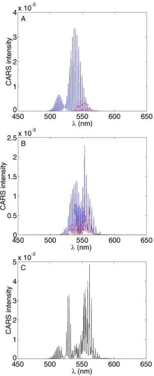
2 . 共4兲As an example, using the parameters relevant to the io-dine experiment 共pump 1= 540 nm, Stokes 2= 565 nm, transform-limited 20 fs FWHM pulses兲, a calculation of the contributions from both diagrams A and B of Fig. 1 at a delay time of ⌬t = −0.790 ps is shown in Fig. 12.
In the top panel of Fig. 12, we show the contribution from diagram A to the CARS spectrum for the various ini-tially populated ground vibrational states. The signals from
X共v
⬙
= 0兲 are in blue 共full line兲, from X共v⬙
= 1兲 in red 共dashed line兲, and from X共v⬙
= 3兲 in black 共dotted line兲 共negligible amount兲. The blue and red combs are shifted with respect to each other by the X-state vibrational energy spacing e, as expected. In the middle panel of Fig. 12, we show the con-tribution from diagram B to the CARS spectrum for the vari-ous initially populated ground vibrational states. We note that whereas diagram A emits preferentially in the high frequency part of the spectrum, diagram B emits preferentially in the low frequency part of the spectrum. Referring to the state labels 共the indices of vibrational states l,k correspond toX-surface; n , m correspond to B-surface兲 given in Fig.1, the major pathway for diagram A l = 1, n = 28, k = 4, m = 36 gen-erates a signal at emission frequency ml=p+ ⍀. For dia-gram B via l = 1, n = 28, k = 1, m = 20, the generated signal
FIG. 11. Log spectrogram of the CARS signal detected at 520 nm, clearly showing the time ordering of the higher frequency terms at⬃176, 250, 325, and 400 cm−1. This demonstrates the high order revival structure: the second
harmonics appear with twice the period of the fundamental, the third har-monic with three times, etc. This confirms the assignment of14,16,18, and101 revivals, as indicated. The101 revivals are the highest reported to date for a molecular wavepacket. For details see the text.
FIG. 10. Fourier transform power spectra of the iodine transients from Figs. 9共a兲–9共c兲. As expected from wavepacket dynamics in an anharmonic poten-tial, the peaks centered near 83 cm−1 correspond to the nearest-neighbor
level spacings whereas as those near 170 cm−1 correspond to the
next-nearest-neighbor level spacings. As the anti-Stokes signal wavelength moves to the blue, the level spacings in the FFT move to the red as expected共i.e., probing higher up in the excited state potential, involving more close lying vibrational levels兲.
emits at the pump frequency nk=p. The bottom panel shows the total signal expected from the coherent sum of the two contributing diagrams.
We note that for diagram B of Fig.1, emission from a process starting in v
⬙
= 0 alone contains several combs shifted by multiples of ⍀ due to the contribution of differentk共i.e., the sample is vibrationally hot兲. Therefore, diagram B should yield broader spectra than diagram A. In general, dia-gram B does not necessarily contribute to the CARS signal for large detuning of the Stokes pulse from the electronic resonance, as discussed in the Introduction. In our case,
how-ever, we deliberately chose a sample which has initially populated vibrationally excited states in X, and a broadband Stokes pulse. Both of these aspects conspire to make dia-gram B significant. The complex structure within the spectra is due to the Franck–Condon factors.
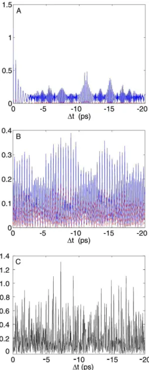
Importantly, the time dynamics along a frequency cut are also different for diagrams A and B. This can be seen from Fig.9 where panels共A兲–共C兲 reflect predominantly the con-tributions from diagram A whereas panel 共D兲 reflects that predominantly of diagram B. As opposed to diagram A, dia-gram B does not show any clear revival structures. The rea-son for this can be understood by considering Eqs.共A15兲and
共A16兲 from the Appendix. By choosing a frequency cut, we select a certain transition due to the resonance energy denominator. The delay-dependent phase is the same for both diagrams but the resonance energy denominators are differ-ent. Therefore, if we choose a frequency cut for diagram B, we strongly limit the number of n contributing to the signal 关see Fig. 1 and Eq. 共A16兲兴. For a transition starting from the ground vibrational state X共l=1兲, we predominantly go to k = 1 which uniquely determines the n contributing to the sum. No wonder one does not see revivals—there is nothing to revive! The emission from diagram A, on the other hand, does not come from the n-levels. Therefore se-lecting a frequency cut does not limit the number of n-levels involved and, therefore, the coherent excitation of these lev-els results in the usual wavepacket revival structure. Since the two diagrams emit in different frequency regions, by making the appropriate frequency cuts as shown in Fig. 9, we are able to isolate signals due to diagram A alone.
We now consider two extremal frequency cuts, at 515 and 550 nm, using the pole approximation39 to calculate the two-photon matrix elements 共see the Appendix兲. As dis-cussed above, the high frequency part of the spectrum is dominated by the signal coming from diagram A. In Fig.13
we show contributions from the two diagrams and for all initially populated vibrational levels. For 515 nm, the signal mostly comes from diagram A for v
⬙
= 0. The signal from diagram B shows little time structure but it does not signifi-cantly contribute to the total signal at 515 nm. Therefore, the canonical wavepacket revival structures can be observed. The situation changes dramatically for the 550 nm frequency cut shown in Fig.14. In this case, diagram B dominates the contribution and the overall time dynamics does not show wavepacket revivals.In our experiments, a pump wavelength of 540 nm means that at the second pump interaction, the wavepacket is projected onto the dissociative continuum of the B-state. Consequently, in calculating the third order susceptibility, one has to both sum over bound state and integrate over continuum contributions. Faeder et al.10did a thorough study of the situation when probing both above and below this threshold. These authors showed how anomalous peaks in the frequency spectrum found only when probing above the dissociation threshold could be assigned as polarization beats. The polarization generated from initial state v
⬙
= 0 in one molecule and v⬙
= 1 in another gives rise to two polar-izations Pi共兲 and Pi⬘共兲. In the case of probing below the threshold, these polarizations consist of narrow,nonoverlap-FIG. 12.共Color online兲 Calculated contribution of different diagrams. Delay time ⌬t = −0.790 ps, decoherence time 0.4 ps. The top panel shows contri-bution of diagram A, starting from different vibrational levels关full v⬙= 0, dashed v⬙= 1, and dotted v⬙= 2共very small signal兲兴. The central panel shows the contribution of diagram B, and shown in the bottom panel is the total spectrum. Details of the calculation of these are given in the Appendix.
ping lines, resulting in little interference in the resulting sig-nal spectrum when the fields generated are squared on the detector. When probing above threshold, however, the polar-izations will be short lived共i.e., spectrally broad兲 and over-lap well, giving rise to large interferences 共polarization beats兲. Starting from a vibrationally hot sample, the signal from a CARS experiment ending above the dissociation threshold after the second pump interaction would therefore be modulated by the splitting between v
⬙
= 0 and v⬙
= 1 in theground state. Comparing our results with Faeder et al., we see in Fig.8 these same sidebands共marked *兲 on the main peak in the Fourier transform power spectra and therefore assign these peaks to this effect.
Finally, we also investigated wavepacket dynamics as probed by ultrashort pulse CARS spectroscopy in bromine and iodine bromide. An example of the CARS signal from bromine is shown in Fig. 15. As shown, we again observe vibrational wavepackets in both ground and excited states of
FIG. 13. 共Color online兲 Delay time dependence of the CARS signal at the signal wavelength 515 nm. The top panel shows the CARS signal corre-sponding to diagram A, calculated using Eq.共A20兲, starting from vibrational levels v⬙= 0共full line兲, v⬙= 1共dashed兲, and v⬙= 2共dotted兲 共very small sig-nal兲. The CARS signal corresponding to diagram B, calculated using Eq. 共A22兲, is shown in the middle. The panel at the bottom shows the coherent sum of the two diagrams. All contributions were calculated using the pole approximation.
FIG. 14. 共Color online兲 Delay time dependence of the CARS signal at the signal wavelength 550 nm. The top panel shows the CARS signal corre-sponding to diagram A, calculated using Eq.共A20兲, starting from vibrational levels v⬙= 0共full line兲, v⬙= 1共dashed兲, and v⬘= 2共dotted兲 共very small sig-nal兲. The signal corresponding to diagram B, calculated using Eq.共A22兲, is shown in the middle. The panel at the bottom shows the dynamics for the coherent sum of the two diagrams. All contributions were calculated using the pole approximation.
bromine. It should be mentioned that this result agrees very well with earlier results40 except that these researchers did not observe ground state wavepacket dynamics due to the narrower bandwidths of their laser pulses. A typical section of the CARS data for iodine bromide is shown in Fig.16. We again see a vibrational wavepacket in the ground electronic state at positive time delays. Interestingly, despite the excep-tional signal-to-noise ratio, we see absolutely no sign of an excited state wavepacket signal. This is surprising because earlier pump-probe experiments on iodine bromide based on time-resolved photoionization32 showed very clear excited state wavepacket dynamics in IBr, at the same wavelengths employed here. We note that, distinct from iodine and bro-mine, iodine bromide is predissociative in this wavelength range and undergoes interesting spin-orbit induced nonadia-batic dynamics.32In our opinion, this intriguing result merits
more consideration as it addresses issues relating to the role of excited state electronically nonadiabatic processes in gen-erating the CARS signals. We note that at both positive 共ground state兲 and negative 共excited state兲 time delays, the emitted third order polarization originates from the same set of continuum states. We speculate that the panoply of elec-tronic states in the vicinity of the IBr B-state may lead to a rapid electronic dephasing of the initially created wave-packet, diminishing the excited state signal. However, this clearly requires more study.
V. CONCLUSION
Ongoing worldwide efforts in laser technology research lead to increasingly ultrashort visible light pulses. The high intensity but short duration of these pulses makes them ideal for various forms of nonlinear optical spectroscopy and these are now applied to problems such as molecular dynamics in condensed phases. We discussed the use of such ultrashort pulses for time- and frequency-resolved CARS experiments. The very broad bandwidths of these ultrashort pulses, how-ever, introduce potential complications due to the possible spectral overlap, and therefore interference, of other third order processes contributing to the signal. These were illus-trated schematically in Fig.1. Furthermore, for complex sys-tems and/or environments, the possibility of having a broad distribution of initial states compounds these complications. As it may be difficult to discern these various contributions in the dynamics of an uncharacterized system, it is therefore valuable to consider their effects in a simple model system. In order to explicitly illustrate these issues in the most transparent manner, we chose gas phase molecular iodine as a model system. We employed a new achromatic dispersion-free, polarization maintaining time- and frequency-resolved CARS spectrometer together with sub-25 fs pump and Stokes laser pulses, and a heatable sample cell. We also de-veloped a simple analytical model, based on the pole ap-proximation, which allows one to quickly evaluate various competing contributions to the third order signal. This model allowed us to disentangle the contributions from the various diagrams and to discern the role of the different initially populated共vibrational兲 states in the heated sample.
This study illustrates how some care may be required when applying ultrashort pulse NLO spectroscopies such as CARS to more complex larger molecules in possibly com-plex environments, where the spectral and time dependence of the different third order contributions may be unknown. In order to most transparently reflect the desired molecular dy-namics in the third order signals, it is important that experi-ments are designed such that a single diagram dominates the signal. The choices of wavelengths, bandwidths, and the tim-ing of the three pulses involved in the process are the param-eters that can be adjusted in order to achieve this selectivity.
ACKNOWLEDGMENTS
A.S.M. is supported by a VKR grant and S.G. acknowl-edges financial support from the Deutsche Akademie der Naturforscher Leopoldina, Award No. BMBF-LPD 9901/8-139. A.S. would like to thank Dr. Michael Schmitt共Jena兲 for
FIG. 15. A section of the CARS data for Br2at 543 nm, where the signal
would be expected to be strongest based on the center wavelength of the pulses used. For negative共positive兲 delays the signal probes a vibrational wavepacket in the excited共ground兲 electronic state.
FIG. 16. A section of the CARS data for IBr at 520 nm, where the signal would be expected to be strongest, based on the center wavelength of the pulses used. For positive delays the signal probes a vibrational wavepacket in the ground electronic state. At negative delays no signal is observed. For a discussion, see the text.
many helpful discussions and Dr. T. Siebert共Berlin兲 for help in the initial phases of this experiment. We thank Doug Mof-fatt for technical assistance.
APPENDIX: AN ANALYTICAL MODEL
In this section we derive analytical formulas for the CARS process using standard time-dependent perturbation theory for the density matrix.7 Atomic units共a.u.兲 are used throughout. Following the notation of Ref. 10, we consider the Hamiltonian of a molecule Hˆmol with two electronic states, g and e:
Hˆmol=
兺
l兩gl典具gl兩gl+
兺
n兩en典具en兩en. 共A1兲 We describe the coupling to the laser field in the rotating wave approximation: Vˆ = −ˆ+E共t兲 −ˆ−E*共t兲, 共A2兲 ˆ+ =
兺
ln 兩en典具gl兩nl, 共A3兲 ˆ− =兺
ln 兩gl典具en兩ln. 共A4兲Here n, l indicate the adiabatic rovibrational eigenstates, and nl=具en兩ˆ兩gl典. The laser field E共t兲 in Eq.共A2兲 is specified as follows:
E = E1共t兲 + E2共t兲 + E3共t兲, 共A5兲
Ei共t兲 = E0e−共t − ti兲
2/22e−ii共t−ti兲+ikir, 共A6兲
where i = 1 describes the first pump pulse, i = 2 describes the Stokes pulse, and i = 3 describes the second pump pulse, = FWHMt/2
冑
ln 2, and FWHMtis the full width at half maxi-mum of the pulse intensity.The perturbation theory for the density operator yields
i˙
⬘
共q兲=关Vˆ⬘
,⬘
共q−1兲兴. 共A7兲 Here the density operator⬘
共t兲 and the operator for the in-teraction with the laser field are written in the inin-teraction representation:ˆ
⬘
共t兲 = eiHˆmoltˆ e−iHˆmolt, 共A8兲
Vˆ
⬘
共t兲 = eiHˆmoltVˆ e−iHˆmolt. 共A9兲 Within this approach the induced dipole moment describing the qth order polarization can be written as具d␣共t兲典共q兲= iq
冕
dt1¯冕
dtq共t − t1兲 ¯共t − tq兲⫻ Sp兵关¯关V
⬘
共t兲,V⬘
共t1兲兴, ... ,V⬘
共tq兲兴其, 共A10兲 where is the unperturbed density operator. The function 共t兲共t兲 = e−␥t 共t ⬎ 0兲 共A11兲
共t兲 = 0 共t ⬍ 0兲 共A12兲
is introduced to take into account the casuality and inevitable damping ␥due to the reasons discussed above.
The CARS process is driven by the third order polariza-tion induced in the medium P共3兲= N具d典共3兲, where N is the density of molecules in the medium. For 具d典共3兲 the triple commutator in Eq. 共A10兲 gives rise to eight terms corre-sponding to eight diagrams described in detail in Ref.10共see Fig. 3 of Ref.10兲. In our case, when the pump pulse does not overlap with the Stokes/pump pulse pair, only diagrams A–E shown in Fig. 1survive. In the following we show the cor-responding contributions of the induced dipoles obtained us-ing Eq. 共A10兲 with q = 3. We will not consider rotational degrees of freedom and, for convenience, omit the electronic indices g, e for the frequencies and matrix elements. There-fore, it is useful to keep in mind that l, k numerate vibrational states on the X-surface and m, n numerate vibrational states on the B-surface.
The negative delay times, when the first pump pulse ar-rives before the Stokes/pump pulse pair 共excited state CARS兲, correspond to diagram A. Consequently, one obtains for dA共t,兲: dA共t,兲 = 2i
兺
l,m,n,k lle−inleilnt共l,m,n,k兲E1共nl兲 ⫻冕
d⬘
d⬙
E2共⬘
兲E3共⬙
兲ei共⬘−⬙兲t 共⬘
+kn− i␥兲共⬘
+mn−⬙
− i␥兲 + c.c. 共A13兲Hereis a delay time between the arrival of the pump pulse and Stokes/pump pulse pair, 共= − ⌬ t兲, ij=i−j and 共l,m,n,k兲⬅lmnlknmk. The sum over l accounts for the fact that several vibrational states in the ground electronic surface can be initially incoherently populated. The corre-sponding weight of these states is given by the diagonal el-ements of the equilibrium density matrix determined from
the Boltzmann distribution共see below兲.
E1共兲, E2共兲, and E3共兲 represent the Fourier transforms of the laser pulses specified in Eq. 共A6兲. In deriving Eq.
共A13兲, we assumed that the pump pulse does not overlap with the Stokes/pump pulse pair and extended the upper limit of the corresponding time integral to infinity. This explains the appearance of the pump pulse Fourier components This article is copyrighted as indicated in the article. Reuse of AIP content is subject to the terms at: http://scitation.aip.org/termsconditions. Downloaded to IP:
E1共nl兲 at the frequencies of the corresponding transitions nl. The emission spectrum is calculated by performing the Fourier transform over t:
dA共,兲 = 1 2
冕
dt d A共t,兲eit 共A14兲 and yields dA共,兲 = 2i兺
l,m,n,k lle−inl共l,m,n,k兲E1共nl兲 ⫻冕
d⬘
E2共⬘
兲E3共ln+⬘
+兲 共⬘
+kn− i␥兲共ml−− i␥兲 + c.c. 共A15兲 The integral over ⬘
in Eq. 共A15兲 describes both resonant and nonresonant populations of the intermediate level k, leading to the real populations in m. The phenomenological damping factor␥ reflects phase decoherence 共transverse re-laxation兲. The relaxation of population 共longitudinal relax-ation兲 is negligible and is not considered here.Analogously, one obtains for dB共,兲, corresponding to the diagram B: dB共,兲 = − 2i
兺
l,m,n,k lle−inl共l,m,n,k兲E1共nl兲 ⫻冕
d⬘
E2共⬘
兲E3共⬘
+−nl兲 共ml−⬘
+ i␥兲共+kn+ i␥兲 + c.c. 共A16兲 This expression is valid for both positive and negative delay times: diagrams B and E yield equivalent results, dB共,兲 = dE共, −兲. However, this does not mean that the resulting dynamics will be the same: the phase factors for d共B兲and d共E兲 have opposite signs.For positive delay times共ground state CARS兲, when the pump/Stokes pulse pair arrives before the second pump pulse, the dipole moment corresponding to diagram C,
dC共,兲, 共= + ⌬ t兲, is given by dC共,兲 = 2i
兺
l,m,n,k llei共lk+兲共l,m,n,k兲E3共lk+兲 ⫻冕
d⬘
E2共lk+⬘
兲E1共⬘
兲 共⬘
−nl+ i␥兲共ml−− i␥兲 + c.c. 共A17兲 In a similar fashion, the dipole moment, dD共,兲, corre-sponding to diagram D, can be found:dD共,兲 = − 42i
兺
l,m,n,k kk共k,l,m,n兲 ⫻E1共mk兲E2共nk兲E3共nm+兲 共+lm+ i␥兲 ei共nm+兲+ c.c. 共A18兲 In deriving Eq. 共A18兲, we assumed that the pump/Stokes pulse pair does not overlap with the delayed pump pulse and extended the upper limit of the corresponding time integral to infinity. This explains the appearance of the pump andStokes pulse Fourier components E1共mk兲 and E2共nk兲 at the frequencies mk and nk of the corresponding transitions. This diagram probes excited state dynamics.
To calculate transition frequencies and matrix elements in Eqs.共A15兲,共A17兲, and共A16兲, we used electronic potential surfaces from Ref. 21 and transition dipole moments from Ref.41. We consider a 540 nm共1= 0.0843 a.u.兲 pump pulse and 565 nm共2= 0.0806 a.u.兲 Stokes pulse. The pump pulse excites the B ← X transition page in iodine: B共28兲−X共0兲 = 0.0848 a.u.. The detuning between the pulses 共⍀ = 0.0037 a.u.兲 corresponds to the energy difference between
X共4兲=0.004 a.u. and X共0兲=0.0005 a.u. levels in iodine. For the analytical calculations, we used the Fourier images of the pulse envelopes in frequency domain:
Ei共兲 = F关Ei共t兲兴 =
冑
2E0e−共 − i兲22/2
. 共A19兲
For FWHMt= 20 fs, FWHMw= 0.0034 a.u. and therefore the pump pulse can excite nine vibrational states within the FWHMof the pulse bandwidth: B共33兲−B共24兲=0.0034 a.u. The same bandwidth was chosen for the Stokes pulse. In our calculations, we included 40 vibrational levels in the X-state and 54 vibrational levels in the B-state. For the temperature chosen in the experiment 共360 K corresponding to 0.001 a.u.兲, three vibrational states in the X-state were ini-tially populated according to the Boltzmann distribution ll = e−El, = 1000 a.u.. We set the phase relaxation width to
␥= 3 ⫻ 10−5 a.u., which corresponds to a decoherence time of 1 /共2␥兲=0.4 ps and partially includes the experimental signal decay due to the rotational anisotropy.
To speed up the calculation of the two-photon transition matrix elements, we used the pole approximation39 leading to the following expression for diagram A:
drA共,兲 = − 22
兺
l,m,n,k lle−inl共l,m,n,k兲E1共nl兲 ⫻E2共nk兲E3共lk+兲 共ml−− i␥兲 + c.c. 共A20兲 for diagram C: drC共,兲 = 22兺
l,m,n,k llei共lk+兲共l,m,n,k兲 ⫻ E3共lk+兲 E2共nk兲E1共nl兲 共ml−− i␥兲 + c.c. 共A21兲 and diagram B 共the same is valid for diagram E, sincedB共,兲=dE共, −兲兲: drB共,兲 = − 22
兺
l,m,n,k lle−inl共l,m,n,k兲E1共nl兲 ⫻ E2共ml兲E3共mn+兲 共+kn+ i␥兲 + c.c. 共A22兲The plots of signal spectrum at a specific time delay for the two contributing diagrams, shown in Fig.12, and the plots of signal strength at a specific wavelength as a function of delay time, shown in Fig.13and Fig.14were based on Eq.共A20兲
for signals diagram A and on Eq.共A22兲for the signals from diagram B.
1
R. Ell, U. Morgner, F. X. Kärtner, J. G. Fujimoto, E. P. Ippen, V. Scheuer, G. Angelow, T. Tschudi, M. J. Lederer, and A. Boiko, and B. Luther-Davies,Opt. Lett. 26, 373共2001兲.
2
I. Jung, F. X. Kärtner, N. Matuschek, D. Sutter, F. Morier-Genoud, Z. Shi, V. Scheuer, M. Tilsch, T. Tschudi, and U. Keller,Appl. Phys. B: Lasers Opt. 65, 137共1997兲.
3
T. Driscoll, G. Gale, and F. Hache,Opt. Commun.110, 638共1994兲.
4
E. Riedle, M. Beutter, S. Lochbrunner, J. Piel, S. Schenkl, S. Spörlein, and W. Zinth, Appl. Phys. B: Lasers Opt. 71, 457共2000兲.
5
T. Kobayashi and A. Shirakawa,Appl. Phys. B: Lasers Opt. 70, S239-S246共2000兲.
6
P. Baum, S. Lochbrunner, and E. Riedle,Appl. Phys. B: Lasers Opt. 79, 1027共2004兲.
7
S. Mukamel, Principles of Nonlinear Optical Spectroscopy共Oxford Uni-versity Press, Oxford, 1995兲.
8
V. V. Lozovoy, B. I. Grimberg, E. J. Brown, I. Pastirkz, and M. Dantus, J. Raman Spectrosc. 31, 41共2000兲.
9
T. Siebert, M. Schmitt, A. Vierheilig, G. Flachenecker, V. Engel, A. Materny, and W. Kiefer,J. Raman Spectrosc. 31, 25共2000兲.
10
J. Faeder, I. Pinkas, G. Knopp, Y. Prior, and D. J. Tannor,J. Chem. Phys. 115, 8440共2001兲.
11
T. Chen, V. Engel, M. Heid, W. Kiefer, G. Knopp, A. Materny, S. Meyer, R. Pausch, M. Schmitt, and H. Schwoerer, and T. Siebert, J. Mol. Struct.
480–481, 33共1999兲.
12
R. M. Bowman, M. Dantus, and A. H. Zewail,Chem. Phys. Lett. 161, 297共1989兲.
13
M. Gruebele and A. H. Zewail,J. Chem. Phys. 98, 883共1993兲.
14
I. Fischer, D. M. Villeneuve, M. J. J. Vrakking, and A. Stolow,J. Chem. Phys. 102, 5566共1995兲.
15
H. Stapelfeldt, E. Constant, and P. Corkum,Phys. Rev. Lett. 74, 3780 共1995兲.
16
M. Schmitt, G. Knopp, A. Materny, and W. Kiefer,Chem. Phys. Lett. 270, 9共1997兲.
17
M. Gutmann, D. M. Willberg, and A. H. Zewail,J. Chem. Phys.97, 8037 共1992兲.
18
M. Karavitis, D. Segale, Z. Bihary, M. Pettersson, and V. A. Apkarian, Low Temp. Phys. 29, 814共2003兲.
19
G. Flachenecker, P. Behrens, G. Knopp, M. Schmitt, T. Siebert, A. Vier-heilig, G. Wirnsberger, and A. Materny, J. Phys. Chem. A 103, 3854 共1999兲.
20
G. Knopp, I. Pinkas, and Y. Prior,J. Raman Spectrosc. 31, 51共2000兲.
21
S. Gerstenkorn and P. Luc, Atlas du Spectre d’Absorption de la Molecule
d’Iode共CNRS II, Paris, 1978兲.
22
J. H. Eberly, N. Narozhny, and J. J. Sanchez-Mondragon,Phys. Rev. Lett. 44, 1323共1980兲.
23
I. S. Averbukh and N. Perelman,Phys. Lett. A 139, 449共1989兲.
24
O. Knospe and R. Schmidt,Phys. Rev. A 54, 1154共1996兲.
25
C. Leichtle, I. S. Averbukh, and W. P. Schleich,Phys. Rev. Lett.77, 3999 共1996兲.
26
V. A. Ermoshin, M. Erdmann, and V. Engel,Chem. Phys. Lett. 356, 29 共2002兲.
27
T. Lohmüller, V. Engel, J. A. Beswick, and C. Meier, J. Chem. Phys. 120, 10442共2004兲.
28
H. Katsuki, H. Chiba, B. Girard, C. Meier, and K. Ohmori,Science 311, 1589共2006兲.
29
A. Stolow, M. J. J. Vrakking, and D. M. Villeneuve,Phys. Rev. A 54, R37共1996兲.
30
I. S. Averbukh, A. Stolow, M. J. J. Vrakking, and D. M. Villeneuve,Phys. Rev. Lett. 77, 3518共1996兲.
31
M. J. J. Vrakking, D. M. Villeneuve, and A. Stolow,J. Chem. Phys.105, 5647共1996兲.
32
M. Shapiro, M. J. J. Vrakking, and A. Stolow,J. Chem. Phys. 110, 2465 共1999兲.
33
S. Meyer, M. Schmitt, A. Materny, W. Kiefer, and V. Engel,Chem. Phys. Lett. 301, 248254共1999兲.
34
S. Meyer, M. Schmitt, A. Materny, W. Kiefer, and V. Engel,Chem. Phys. Lett. 281, 332共1997兲.
35
M. Schmitt, G. Knopp, A. Materny, and W. Kiefer,Chem. Phys. Lett. 280, 339共1997兲.
36
T. Siebert, M. Schmitt, T. Michelis, A. Materny, and W. Kiefer,J. Raman Spectrosc. 30, 807共1999兲.
37
R. Maksimenka, B. Dietzek, A. Szeghalmi, T. Siebert, W. Kiefer, and M. Schmitt,Chem. Phys. Lett. 408, 3743共2005兲.
38
I. Fisher, M. J. J. Vrakking, D. M. Villeneuve, and A. Stolow,Chem. Phys. 207, 331共1996兲.
39
M. V. Fedorov, Interaction of Intense Laser Light With Free Electrons 共Routledge, London, 1991兲.
40
M. Schmitt, G. Knopp, A. Materny, and W. Kiefer,J. Phys. Chem. A 102, 4059共1998兲.
41
J. Tellinghuisen,J. Chem. Phys. 106, 1305共1997兲.