A Time-independent Deformer for Elastic-rigid Contacts

HAL Id: hal-02541299

https://hal.inria.fr/hal-02541299

Submitted on 15 Apr 2020

HAL is a multi-disciplinary open access

archive for the deposit and dissemination of

sci-entific research documents, whether they are

pub-lished or not. The documents may come from

teaching and research institutions in France or

abroad, or from public or private research centers.

L’archive ouverte pluridisciplinaire HAL, est

destinée au dépôt et à la diffusion de documents

scientifiques de niveau recherche, publiés ou non,

émanant des établissements d’enseignement et de

recherche français ou étrangers, des laboratoires

publics ou privés.

Camille Brunel, Pierre Bénard, Gael Guennebaud, Pascal Barla

To cite this version:

Camille Brunel, Pierre Bénard, Gael Guennebaud, Pascal Barla. A Time-independent Deformer for

Elastic-rigid Contacts. Proceedings of the ACM on Computer Graphics and Interactive Techniques,

ACM, 2020, 3 (1), pp.21. �10.1145/3384539�. �hal-02541299�

A Time-independent Deformer for Elastic-rigid Contacts

CAMILLE BRUNEL,

PIERRE BÉNARD,

GAËL GUENNEBAUD,

PASCAL BARLA,

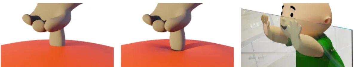
Fig. 1. Time-independent elastic deformations. Left: a rigid finger and an elastic balloon are intersecting in the initial configuration. Center: result of our deformer, the deformed balloon surface exhibits volume preserving bulges with C1continuity. Right: two hands pressing against a window. The right hand is in simple intersection (the fingers are inside the window, while the palm has traversed it). The left hand has been deformed with our technique to convey plausible contact and bulging effects.

We introduce a new tool that assists artists in deforming an elastic object when it comes in intersection with a rigid one. As opposed to methods that rely on time-resolved simulations, our approach is entirely based on time-independent geometric operators. It thus restarts from scratch at every frame from a pair of objects in intersection and works in two stages: the intersected regions are first matched and a contact region is identified on the rigid object; the elastic object is then deformed to match the contact while producing plausible bulge effects with controllable volume preservation. Our direct deformation approach brings several advantages to 3D animators: it provides instant feedback, permits non-linear editing, allows for the replicability of the deformation in different settings, and grants control over exaggerated or stylized bulging effects.

CCS Concepts: • Computing methodologies → Procedural animation; Mesh geometry models. Additional Key Words and Phrases: geometry processing, deformations, animation

ACM Reference Format:

Camille Brunel, Pierre Bénard, Gaël Guennebaud, and Pascal Barla. 2020. A Time-independent Deformer for Elastic-rigid Contacts. Proc. ACM Comput. Graph. Interact. Tech. 3, 1 (May 2020), 21 pages. https://doi.org/10. 1145/3384539

1 INTRODUCTION

Many objects of our everyday surroundings exhibit elastic behaviors when put in contact with more rigid objects, e.g., a cat walking on a pillow, a hand pressed on a window, or a soft ball bouncing on a goalpost. They most notably tend to squash inside the contact region and to bulge as their volume gets redistributed outside of it. Such squashing and bulging effects are essential to

Authors’ addresses: Camille Brunel, [email protected], Inria Bordeaux Sud-Ouest, France; Pierre Bénard, pierre. [email protected], LaBRI (UMR 5800, CNRS, Univ. Bordeaux), France; Gaël Guennebaud, [email protected], Inria Bordeaux Sud-Ouest, France; Pascal Barla, [email protected], Inria Bordeaux Sud-Ouest, France.

© 2020 Association for Computing Machinery.

This is the author’s version of the work. It is posted here for your personal use. Not for redistribution. The definitive Version of Record was published in Proceedings of the ACM on Computer Graphics and Interactive Techniques, https: //doi.org/10.1145/3384539.

communicate plausible deformations in a variety of contexts, such as animated films, visual effects or video games. They are particularly important in character animation, for instance when artists set out to convey actions of a character on the environment or on another character (e.g., grabbing, pushing, pressing, etc). Deformations in contact are thus frequently needed in practice; yet existing computer graphics tools remain of limited control for artistic use.

The classical approach to address this problem relies on the physics of elastic objects by explicitly simulating their behavior (e.g., [Nealen et al. 2006]). The obvious advantage of these approaches is their physical accuracy, provided artists manage to find the physical parameters that yield the sought-for behavior. In practice, this requires extensive training and skills, and frequent trials and errors even for a simulation expert. Physical accuracy may even be a drawback for productions that aim for cartoony, exaggerated deformations [Lasseter 1987]. Besides, the major limitation of simulations in an interactive context is their dependence on time which prevents their use at the rigging or animation stage, while artists are manipulating the 3D assets.

For character animation, physically-based approaches [Gao et al. 2014; McAdams et al. 2011; Smith et al. 2018; Teng et al. 2014] circumvent this limitation using time-independent quasi-static simulations — even though distant contact deformations still depend on the path taken to the colliding state — but they are highly computationally demanding (0.5 to 5 sec per frame) since a large set of non-linear equations must be solved iteratively, and are thus still unsuitable for live user interaction. Alternatively, using simpler position-based models [Bender et al. 2015; Bouaziz et al. 2014], local collisions can be supported at interactive rates [Abu Rumman and Fratarcangeli 2015; Deul and Bender 2013; Komaritzan and Botsch 2018]. Even though these methods may help fixing skinning artifacts, such as local surface self-intersections near joins, they are not designed for distant contacts between body parts or with external objects.

The alternative solutions, at the opposite end of the methodological spectrum, are manual, fully artist-controlled approaches such as those based on blend shapes, free-form [Nieto and Susín 2013; Sederberg and Parry 1986] or pose space deformation [Lewis et al. 2000]. Their main advantage is their simplicity: they provide instant feedback to artists, who are then in charge of producing compelling deformations. In practice, bulging effects remain scarce in production because the task of sculpting deformations and animating them by hand requires a significant amount of time, even for accomplished artists. Even worse, each deformation is specific to the shape of objects and their actual contacts, hence it cannot be reused in different situations (e.g., from shot to shot).

For character animation, specific skinning techniques ensure local or global preservation of the volume [Kavan and Sorkine 2012; Rohmer et al. 2009; von Funck et al. 2008], and one can even avoid surface self-intersections [Angelidis and Singh 2007], but it requires temporal integration and offers limited, indirect artistic control through painted weights. Implicit skinning [Vaillant et al. 2013, 2014] can also handle local collisions of the skin between neighboring articulations without resorting to simulation thanks to its implicit volumetric representation of the character. Yet its gradient-based operators are difficult to art-direct, and distant contacts are too expensive to handle at interactive rates.

To the best of our knowledge, only a few alternative approaches have been proposed in the general context of 3D elastic objects. Among them, the method of Aldrich et al. [2011] automatically updates a cage-based deformer to resolve the collision of a rigid object with an elastic one, while approximately preserving the volume enclosed by the cage. It provides some control over the stiffness of the elastic object and is free of temporal dependencies, but it only achieves interac-tive performances with an expensive, iterainterac-tive GPU algorithm. In addition, since it requires an intermediate volumetric representation, the method leads to global, coarse deformations rather than localized surface bulging. The geometric framework of Harmon et al. [2011] resolves surface intersections interactively during geometric modeling, but it involves a computationally extensive

numerical constrained optimization and lacks artistic controls of the deformation. The concurrent method of Li and Barbič [2019] showed improved results for the specific case of handle-based As-Rigid-As-Possible (ARAP) deformation [Wang et al. 2015], but otherwise suffers from similar limitations.

Our objective in this paper is to develop a deformation tool that assists the artist by managing contacts and bulging effects in an art-directable way. A seamless integration in animation workflows requires: (1) that the tool provides instant feedback to the artist; and (2) that deformations are time-independent to allow non-linear editing. For plausible bulging effects, it is also desirable that the method preserve volume to some extent; even though artistic controls should also be possible to explore more exaggerated behaviors. However, to make this problem tractable, we need to make one major assumption: during the collision, we will consider that one object region is elastic while the other one is fully rigid.

Procedural deformers, such as the Autodesk Maya©_{plugin iCollide or the Cinema4D}©_collision deformer, partially fullfil these objectives by offering instant deformation with control of the bulge profile. As described by Wang [2015], they proceed in two main steps. First, they detect the points of the elastic object that are inside the rigid object, and project them to their closest position on the rigid surface, hence fully collapsing the intersection region. Second, the elastic surface outside the intersection region is deformed along its normal field proportionally to the interpenetration depth. Since the volume in intersection is not considered, the tool may yield unplausible results. Moreover, with this approach the whole pair of surfaces in intersection are kept in contact: as a result, effects as shown Figure 1 cannot be achieved, and instabilities might occur during animation, requiring artists to adjust parameters through time, which is impractical.

In comparison, our approach achieves plausible bulging deformations for any pair of elastic and rigid objects in intersection (see Figure 1), with instant feedback and no time dependency, by relying entirely on geometric operations. It first identifies the region of the elastic object that will remain in contact with the rigid one, taking into account their respective shapes and stiffness. The surface of the elastic object is then deformed instantaneously with a direct method to convey bulging effects. The deformation is obtained as a 1D displacement along a diffused direction field and the instantiation of a 1D profile curve that allows artistic bulging control, from no to full volume preservation and even exaggeration. The resulting deformation both looks plausible and continuous in space and time even though each frame is processed independently. Our approach opens new avenues for the animation of elastic objects in contact: editing may be performed non-linearly, similar deformations may be replicated in different contexts without requiring tedious manual adjustments, and many artistically-driven effects can be easily accomplished by tweaking the profile curve.

2 OVERVIEW

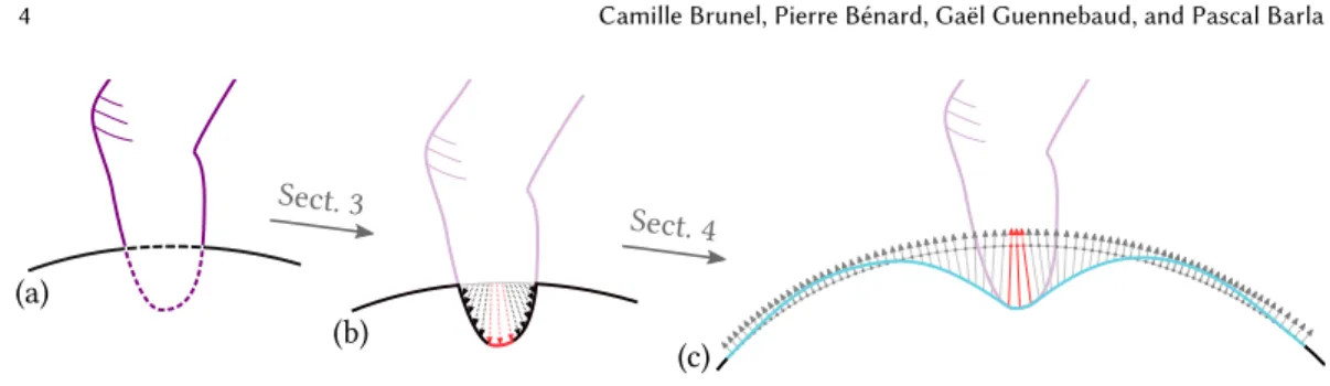
Our approach considers a pair of objects in intersection as illustrated in Figure 2(a): one object is flagged as rigid (in purple) and the other as elastic (in black). The process restarts from scratch at every frame and works in two main stages.

In the first stage, detailed in Section 3, we first determine the regions in intersection (dashed lines in Figure 2(a)), and match them with each other in parametric space. This mapping enables us to project the elastic surface onto the rigid one in this region as illustrated in Figure 2(b); we then identify the contact zone (in red), which corresponds to the points of the elastic surface that will stay in contact with the rigid object after deformation. Our algorithm computes this contact zone by implicitly taking into account the geometry of the rigid and elastic objects, the depth of penetration, and a user-controlled pseudo-stiffness parameter. Our solution is motivated by the empirical observation that the stiffer the elastic object is, the smaller the contact region should be.

Sect. 3

(a)

(b) _(c)

Sect. 4

Fig. 2. Overview of our approach. (a) Our operator restarts from scratch at every frame with a pair of objects – one rigid (in purple), the other elastic (in black) – and computes the intersection between them (dashed lines). (b) The elastic object is then projected on the rigid one inside the intersection zone (solid black line); a contact zone (in red) is established based on a pseudo-stiffness parameter. (c) The extent of the deformation, a direction field (arrows) and a pair of scalar magnitude and slope fields (not shown) are computed using diffusion processes; these are used to guide the displacement of the initial elastic surface (in light gray) toward its final shape (in light blue).

In a second stage, we aim at deforming the neighborhood of the contact zone in a plausible way, as described in Section 4 and visualized in Figure 2(c). The extent of the deformation is bounded by user-controlled pseudo-geodesic distance from the boundary of the contact region. The deformed surface is obtained as the displacement of the initial surface along a smooth direction field d. More formally, the final position p′

i of each point pi on the initial surface is thus defined as:

p_i′ = pi+ Hai,si(ui) di. (1)

The displacement magnitude is controlled by a 1D profile curve H evaluated along a one-dimensional radial parametrization ui ∈ [0, 1]. Intuitively, uilocates a point of the elastic surface along smoothed geodesics going from the contact zone to the external boundaries of the deformable region. It is obtained through the normalization of the pseudo-geodesic distance used to compute the extent of the deformation. The shape of the profile curve H is parametrized by the amplitude ai and slope si at u = 0. Those degrees of freedom are required to respectively ensure C0_{and C}1_continuity with the contact zone. For similar reasons, the direction field d needs to smoothly interpolate the matching directions at the boundary of the contact zone, and the original surface normals at the external boundary of the deformable region. Those three fields (a, s and d) are carefully computed through some variants of harmonic diffusion.

Finally, the shape of this profile can also be automatically optimized to ensure pseudo-volume conservation, thus producing bulging effects. This effect can be cancelled or even exaggerated through a single user-controllable parameter. We provide the pseudo-code for the full algorithm in Appendix C. Part 1 corresponds to the contact zone definition and Part 2 to the deformation.

Remarks.Whereas several approaches could be imagined to compute the deformation, the com-bined use of a direction field and a 1D displacement profile exhibits several compelling properties: (1) Constraining the deformation along a predetermined direction field is key to define a linear

pseudo-volume preservation term.

(2) This approach is direct and does not involve any iteration nor non-linear energies as would be required with, for instance, an ARAP-based method (e.g., [Wang et al. 2015]).

(3) Our approach opens the door to many user-controlled effects through the simple edition of a 1D profile curve.

(a) rs 2rs rs p′_i ci p′ n′_i (b) li p_i′ p′_j n′ j c(1) α 1 − α n′ i c(0) _c(α) p′ (c)

Fig. 3. Ball testing and sliding in 2D. (a) Contact zones (red and brown solid lines) are identified on the projected elastic surface (black solid line) by testing whether it can fit a ball of a given radius (rs for the

region in red, 2rsfor the one in brown). (b) For a vertex at position p′iwith normal n′i, we test whether any

other vertex p′_{of the elastic mesh is inside the ball with center c}

iand radius rs, excluding all vertices behind

the hyperplane with normal n′

ipassing through the point li. (c) The contact zones extend across edges: for a

vertex at position p′

i with normal n′iinside the contact zone (in dark red) connected to a vertex with position

p′_j with normal n′_joutside this zone (in gray), we search for the smallest parametric location α along this edge such that the associated ball (in red) with center c(α) and radius rs is tangent to another vertex p′of

the elastic mesh (the ball radius is usually much larger than the edge in practical situations).

3 CONTACT ZONE

At each frame, we start from two manifold triangle meshes already in intersection. For performance reasons, we work on open subsets denoted We_{and W}r_{of the elastic and rigid meshes respectively.} Those regions are selected by the user according to the expected spread of the deformation, but it could also be automatically determined as a distance to the intersection region. We further assume that both surfaces are equipped with a continuous 2D parametrization.

3.1 Intersections Detection

We first need to robustly detect the two regions in intersection (Figure 2(a)). For each mesh, we determine the set of edges that are intersected by faces of the other mesh, recording the corresponding intersection points qe_{(resp. q}r_{) in parametric space of the elastic (resp. rigid) mesh.} This computation is accelerated using a standard 3D Axis-Aligned Bounding Box (AABB) tree.

For each edge in intersection, we consider each of its extremities independently and tag it as either interior or exterior based on the normal of its closest intersected face. We eventually propagate the interior tags on both elastic and rigid mesh vertices with a flood fill algorithm to delimit the two regions in intersection. Note that we do not need to insert the intersection points into the meshes. 3.2 Regions Mapping

We now aim to define a mapping between these two interior regions to be able to project the elastic surface onto the rigid one (arrows in Figure 2(b)). We construct this mapping in parametric space leveraging the constraints provided by the intersection points. We proceed in two steps. First, we compute the global affine transformation A that minimizes, in the least-squares sense, the distance between every pair of intersection points expressed in the two parametrizations, i.e., minimizing:

Õ k

∥ek∥2, with ek = qr_k−A qe_k.

This global transformation is then further refined locally to enforce the intersection points to match more accurately, i.e., ∥ek∥ = 0, ∀k. To do so, we compute a smooth 2D deformation field g by harmonic diffusion of the error vectors ekover the interior vertices [Botsch and Kobbelt 2004]. As the error vectors ekare defined along edges we cannot use standard Dirichlet conditions. Instead, we include the one ring of outside vertices adjacent to the interior region and introduce the ek targets as linear least-squares constraints as detailed in Appendix A.

At this stage, each interior vertex i of the elastic object knows its parametric location in the rigid object parametrization: qr

i = A qei + gi. To find its 3D position pi′and normal n′ion the rigid surface, we search the face and barycentric coordinates associated to qr

i. To speedup searches, we use a 2D AABB-tree built in parametric space over the rigid mesh.

3.3 Contact Zone Extraction

Eventually we want to identify which part of the elastic surface in intersection will remain in contact with the rigid one after deformation (in red in Figure 2(b)). Inspired by α-shapes [Edelsbrunner and Mücke 1994], we translate the stiffness of the elastic object into the radius rs of a virtual ball that would roll on the interior of the elastic mesh after being projected on the rigid mesh (Figure 3(a)). The contact zone corresponds to the sub-region of the surface accessible by this ball. The larger the ball, the least it can access concavities of the elastic surface, the smaller the contact zone will be. The contact zone will naturally expand as the depth of the intersection grows.

We developed a fast approximation of this test called ball testing. For each vertex with index i of the deformable region in intersection, we check whether any other deformable vertex is inside the ball of radius rs and center ci = p′

i + rsni′; if so, this vertex is not part of the contact zone (Figure 3(b)). This test is accelerated using a 3D AABB-tree, here built over all the projected vertex positions.

However, defining the contact zone at vertices will not allow a smooth temporal evolution of its boundary. To refine it further, we compute the exact contact-boundary points on the outgoing edges of the contact zone by “sliding” the same virtual ball along them until it touches the elastic surface (Figure 3(c)). More precisely, for each edge ij connecting a vertex with index i inside the contact zone to a vertex with index j outside this zone, the ball is defined by the constant radius rs and the linearly interpolated center: c(α) = (1 − α) ci+ α cj, with α ∈ [0, 1] the parametric location along the edge. The exact contact-boundary point corresponds to the smallest α at which the ball is tangent to another vertex p′_{of the elastic mesh. This boils down to solving the quadratic equation:}

∥p′− c(α)∥2−r_s2= 0.

In practice, we perform this test on every vertex contained in the axis-aligned bounding box of the two spheres associated to the extremities of the edge (i.e., with center c(0) and c(1)), leveraging the same 3D AABB-tree. If the edge contains intersection points (Section 3.1), then we clamp α as required to ensure that the contact-zone stays within the intersection. The overall smallest α is stored on the ij edge and denoted later as αij.

As we linearly interpolate the ball centers, the ball can slightly penetrate the deformed surface along the edge as seen in Figure 3(c), thus leading to false detection. Enforcing the ball to remain tangent to the edge would make the problem of finding the optimal α intractable. Moreover, since the points p′_{come from the projection onto a discrete surface, and not a continuous one, the above} tests are sensitive to slight variations of the projection. We address both problems by excluding from ball testing all vertices lying behind an hyperplane of normal n′

i and passing through the point li = p_i′+ λin′_i(Figure 3(b)). Here, λi is chosen as the smallest positive scalar such that the one-ring neighborhood of the current vertex lies in the rejection side of the hyperplane. This effectively excludes the topological one-ring-neighborhood while being compatible with the continuous ball-sliding test: the interpolated hyperplanes are obtained by linear interpolation of their respective normals n′

i, n′j and reference points li, lj.

At the end of this step, the contact zone can be composed of multiple non-connected regions that can smoothly split and merge during the animation. Note that we never need to insert the contact points into the elastic mesh, nor do we have to chain them together, which significantly simplifies computation.

4 DEFORMATION

The objective here is to compute the final position of the elastic surface around the contact region (Figure 2(c)). As formalized in Equation 1, this is accomplished by a pure geometric displacement along a smooth direction field d. The displacement magnitude is controlled by a 1D profile function Hdefined over a 1D radial parametrizationu ∈ [0, 1]. To ensure a smooth transition with the contact region, an adjusted profile Hai,si is instantiated at each vertex piof the deformable region D by

fixing its amplitude aiand slope siatu = 0. Since this information is only known at the contact-zone boundary, we have to diffuse it to the rest of the deformable region yielding the two corresponding smooth scalar fields a and s. Note that si reflects the slope of the displacement in the direction orthogonal to the boundary of the contact region, which is thus unrelated to the gradient of ai. To illustrate that point let us consider a simple symmetric configuration like a rigid sphere colliding an elastic plane. In this case, the amplitude ai along the boundary of the contact zone is expected to be constant, and thus the field a will also be constant over D. Its gradient will be a null vector field, whereas the scalar field s will also be constant over D, because its value will reflect the slope of the sphere on the direction orthogonal to the boundary of the contact region.

The computations of the different ingredients in Equation 1 are described in Sections 4.1 through 4.4 and summarized in Algorithm Part 2, in the order they are computed: first the 1D radial parametrization u, then the direction field d, followed by the guiding amplitude a and slope s fields, and finally the profile instantiation Hai,si with volume conservation.

4.1 Deformable Region Parametrization

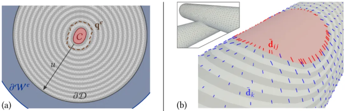
Our 1D parametrization u ∈ [0, 1] of the deformation region is defined as u = ϕ/ϕmax, where ϕ is a scalar field measuring a smoothed geodesic distance to the contact boundary ∂C, and ϕmaxis a user specified maximum geodesic distance controlling the extent of the deformation (Figure 4(a)). Formally, the exterior boundary of the deformable region is defined as the iso-contour ϕ = ϕmax.

Our computation of ϕ is inspired by the state-of-the-art heat-method [Crane et al. 2013], which is a three-steps procedure:

(1) Compute a scalar field v through heat diffusion. (2) Compute the normalized gradient field X = −∇v/∥∇v∥. (3) Solve the Poisson equation ∆ϕ = ∇ · X.

Our approach mostly departs from the original method in the first step. Let us recall that at this stage we work on an open subset We _{of the elastic surface (Figure 4(a)). In such a case, Crane et al.} recommended to compute v as the average of the two heat-diffusion solutions obtained with vanishing Neumann and Dirichlet conditions respectively, which we found too expensive for us. From our experience, Dirichlet conditions alone yield significantly better and stable solutions than natural Neumann conditions, especially if We_{is large enough. Moreover, since we are seeking} for a smooth distance field (implying a very large time-step in the heat-diffusion), it is simpler to consider the solution of the steady state problem:

∆v = 0 with v = 1 on ∂C and v = 0 on ∂We where ∂We_{denotes the exterior boundary of W}e_.

As the contact boundary ∂C is not defined on existing vertices of the mesh, but as a set of points lying on its edges, we implement its respective boundary condition as a set of least-square linear constraints (1−αij)vi+αijvj = 1 for all edges ij crossed by the contact boundary (see Appendix A). To avoid temporal discontinuities when the contact boundary ∂C crosses a vertex, we need to be careful when assembling the Laplacian matrix. The integrals Lij =< ∇φi, ∇φj > of the gradients of the linear basis-function φi have to be computed over the true working region We_.

C qe ∂We (a) u ∂D (b) ¯dij ¯dk

Fig. 4. Visualization of the parametrization and direction field. (a) Top view of the elastic surface in Fig. 1, showing the intersection points qe(in brown), the contact region C, the deformable region boundary ∂D and working region boundary ∂We_{. The radial parametrization u (grey periodic iso-values) is 0 on the contact}

boundary ∂C and 1 on ∂D. (b) A more complex configuration (inset figure). The 2D projection of the direction field onto the surface tangent plane ¯d (in blue) is diffused from the value constraints ¯dij(in red).

pi

pj

αij ∂C

In practice, this means that the three cotangent terms associated with a triangle face overlapping ∂C need to be weighted by the ratio between its area after being cut by ∂C (inset figure, grey region) and its full area.

When solving the Poisson equation in step 3, we reuse the same adjusted cotangent weights to compute the integrated divergences, and the same least-square constraints to ensure that ϕ = 0 on ∂C.

The result of this process is depicted in Figure 4(a). The parametrization respects the boundary constraints, is smooth, almost linear, and radially symmetric when expected.

4.2 Direction field

The direction field along which the elastic surface vertices are displaced is subject to two constraints: (1) it must match the fixed displacements of the contact zone, and (2), for a smooth shape, it should be mostly aligned with the surface normals ni. For each vertex pi of the exterior boundary of the deformable region, we thus impose d(pi) = di = ni. Likewise, for each edge ij crossed by the contact boundary ∂C, we should have:

d(pij)= dij, with dij = pij− p ′ ij ∥pij− pij′∥

,

where pij = (1 − αij)pi + αijpj is the exact boundary point along the edge, and p_ij′ is its projection onto the rigid surface as obtained from the mapping defined in Section 3.2.

ni pi bi ti di ¯di nj Ri(j bj tj pj ¯dj dj ¯Ri(j

To take into account the change of orientation over the surface, we encode each displacement direction di as its 2D projection onto its local tangent plane:

¯di = B⊤ i di,

where the precomputed 3 × 2 matrix Bi = [ti bi]holds a pair of unit and orthogonal tangent vectors (inset figure). Intuitively, ¯di represents how much the direction deviates from its normal in tangent space. This also has the advantage of relaxing the non-linear unit vector constraint during the

diffusion. A direction di is then recovered as: di = Bi ¯di+

q

1 − ∥¯di∥2ni.

This reduction of dimensionality is possible because we assume that the fixed directions at the contact boundary are directed towards the exterior of the deformable surface, which is a reasonable assumption for smooth surfaces (see Section 6).

We interpolate these tangent vectors between the two boundaries using harmonic diffusion and parallel transport. Since two adjacent vectors ¯diand ¯dj are encoded within different tangent frames, the later needs to be parallel-transported before being compared using ¯di− ¯Ri_(j¯dj, where ¯Ri_(jis a 2D rotation encoding the in-plane rotation from j to i.

We pre-compute it as ¯Ri₍j = Bi⊤Ri(jBj where Ri(j is the 3D rotation aligning the normal nj with ni. For efficiency we encode both the tangent vectors and rotations as complex numbers. In practice, the parallel-transport rotations are thus incorporated within the weighted Laplacian matrix by multiplying each off-diagonal element Lijby the unit complex version of ¯Ri(j. We refer to [Knöppel et al. 2013] (their Section 2) for more details on parallel transport and an alternative computation of the transport rotations.

Finally, the linear value constraints ¯d(pij)= ¯dij on the contact-boundary ∂C are introduced in a least-squares sense, as described when computing the scalar field v (Appendix A). A notable difference is that parallel-transport rotations from the edge extremities i and j to the point pijalso need to be included in the constraint matrix. The result of this process is depicted in Figure 4(b). 4.3 Amplitude and Slope Fields Diffusion

The amplitude field a is computed through harmonic diffusion of the displacement magnitudes at the contact boundary ∂C. For each contact boundary edge ij, the expected amplitude is given as aij = ∥pij− p′

ij∥. At a first glance, this problem seems equivalent to the three previous diffusions. There is, however, a fundamental difference that prevents the use of the same numerical scheme. In Sections 4.1 and 4.2, the constraints on ∂C were constant or extremely smooth for d, with maximal variations of the resulting fields in the direction orthogonal to ∂C. In contrast, the value of a may vary greatly along ∂C and the resulting field is expected to be nearly constant in the direction orthogonal to ∂C. In this context, using least-squares linear constraints tends to yield spurious values around vertices linked to multiple constrained edges with very different target values.

We alleviate this difficulty by explicitly computing the expected amplitude of each vertex pj adjacent to a contact-boundary edge ij as the weighted average of the displacement magnitude established in parametric space:

aj = Í i ∈Njαijaij Í i ∈Njαij ,

where Njdenotes the set of adjacent vertices of pj within the contact-zone. The weights αijensure temporal continuity. The amplitude of the remaining vertices is then computed by harmonic diffusion with standard Dirichlet conditions, fixing a along ∂D to the mean amplitude along ∂C. The slope field s is computed using the same weighted average for the vertices adjacent to the contact boundary followed by a standard diffusion process. Beforehand we need to estimate the expected slope sijat each contact-boundary edge, taking into account the values of the parametriza-tion u, direcparametriza-tion field d, and amplitudes a that have been actually computed. For a small u, the profile curve H can be approximated as a linear function depending only on the previously computed amplitude, and the yet unknown slope. Along the edge ij, the displaced position of pj can thus be approximated as a function of its slope value sij:

v2, γ = 1 v3v4v5 0 0.2 0.4 0.6 0.8 1 -1 -0.8 -0.6 -0.4 -0.2 0 0.2 v1, s i= 0 .5 v0 v1, si = 0 v1 ,si =0. 9 v3v4v5 0 0.2 0.4 0.6 0.8 1 -1 -0.8 -0.6 -0.4 -0.2 0 0.2 v1, s i= 0 .5 v0 v2, γ = 1 v2, γ = 0.4 v2, γ = 0 1 3 56 1112

Fig. 5. Profile curves. The control points v0and v5are fixed to ensure surface continuity. The position of v1

is constrained to the circular arc with center (0, −1) and radius 0.2 and fully determined by the slope angle θi at the evaluation vertex i (left). The ordinate of v2is optimized according to the user-defined bulging

parameter γ (right). The abscissas of v2, v3and v4can be edited for additional artistic control of the bulge

position and shape.

pi pij dij pj dj n′ ij ˜pij _˜p j(sij)

As illustrated in the inset figure, we estimate sijsuch that ˜pj lies on the tangent plane of the rigid surface:

(˜pj(sij) −˜pij)⊤nij′ = 0 , where ˜pij = pij+ ajdij, and n′

ijis the normal of the rigid surface at p′

ijobtained through barycentric interpolation.

pi pj pij dij _d j n′ ij p′ ij aj aij

Notice that the target plane is not positioned exactly on the rigid surface. This approximation actually improves stability in cases where ujis extremely small (say < 10-4_{) and the actual value of aj is slightly different than aij. Such a case} would lead to arbitrarily large slope estimates to cope for the tiny gap between aijand aj.

4.4 Profile Curves Instantiation

To instantiate the deformation profiles, we use parametric open uniform cubic 2D B-splines f : t ∈ [0, 1] → (f1(t), f₂(t)) for their smoothness, local control, high flexibility, ease of editing, and ability to generate profiles with a vertical slope at u = 0. The downside of using a parametric curve is that the evaluation of the profile H(u) at a given u involves the inversion of f1:

H (u) = f2(f₁-1(u)) .

In practice, the secant method turned out to be effective enough to make the cost of these inversions negligible compared to the rest of the pipeline.

As illustrated in Figure 5, the shape of the B-spline f is defined by six control points vk, k ∈ {0 . . . 5}, that are automatically adjusted for each vertex i of the deformed surfaces to match

rs = 25, ϕmax= 75 rs = 20, ϕmax= 75 rs = 20, ϕmax= 100

rs = 38, ϕmax= 150 rs = 20, ϕmax= 50 rs = 20, ϕmax= 100

Fig. 6. Test examples. First and third rows: objects in intersection. Second and fourth rows: result of our deformer with default settings. From left to right: A rigid sphere (diameter=50) on an elastic one (diameter=100); two horizontal capsules (diameter=100) colliding perpendicularly and parallelly; an elastic sphere (diameter=100) on a rigid plane, two capsules with different orientations, each taking the role of the elastic object in turn.

the given amplitude ai, slope si, as well as the volume preservation and user-controlled bulging parameters hvand γ :

v0 v1 v2 v3 v4 v5 abscissa (x) 0 0.2 cosθi 1/3 5/6 11/12 1 ordinate (y) −ai ai(0.2 sinθi−1) γ · hv 0 0 0 with θi = tan-1_{(si/ai). The rationale behind the formulas controlling v}

1is depicted in Figure 5(left). Recall that v1must be positioned to satisfy the given slope si, and since it can be arbitrarily large, we need to adjust both its abscissa and ordinate. To do so, we consider a canonical configuration with unit amplitude (by dividing the ordinates by ai) and constrain v1on the circular arc of radius 0.2 centered in (0, −1). The last three control points are aligned with the horizontal axis to ensure C2_{continuity at u = 1.}

Pseudo-volume preservation.As illustrated in Figure 5(right), the ordinate of v2 controls the amount of bulging of the deformation. It is determined as the product of a user-controlled parameter γ allowing to either suppress or exaggerate the bulge, and a scalar value hvwhich is automatically recomputed at each frame to approximately preserve the volume of the elastic object when γ = 1. To

this end, for each vertex pi, we approximate its associated change of volume δVi as the magnitude of its displacement times one third of the area of its adjacent faces, denoted as Ai. The sum of the δVjover the deformable region D is a linear function of hvwhose optimal value is found by equating this sum to the sum of the δVjover the contact zone C:

Õ i ∈C Ai ∥p′_i− pi∥=Õ j ∈D AjHaj,sj(uj) = ©­ « Õ j ∈D Aj Õ k,2 N4 k(tj)ª® ¬ + hv© ­ « Õ j ∈D AjN4 2(tj)ª® ¬ ,

where tj = f₁-1(uj), and N_k4denotes the kthcubic B-spline basis function. The position of the bulge can be artistically controlled by moving the abscissas of v2, v3and v4. Note that we chose to set both γ and hvconstant over the deformable region, but nothing prevents them to vary spatially through user inputs (e.g., spatially-varying weights painted on the surface) or additional constraints. 5 RESULTS

Our method requires the pair of input surfaces to be parametrized. For all our results, we use the boundary-free ARAP parametrization method of Liu et al. [Liu et al. 2008] (10 iterations) initialized with LSCM parametrization [Lévy et al. 2002].

In the following, we indicate values for the three global user-controlled parameters of our deformer: the pseudo-stiffness rs, the extent of the deformation region ϕmaxand the volume conser-vation/exaggeration parameter γ . We use the default profile curve H unless specified otherwise. 5.1 Qualitative evaluation

Test examples.We first evaluate our approach on a few test-cases made of various combinations of sphere and capsule objects. Figure 6 shows five basic, yet challenging, configurations with each time a pair of rigid and elastic objects in intersection followed by the result of applying our deformer. We use γ = 1 throughout. In the last two columns, we have inverted the roles of the objects, which has a notable effect on the size of the contact zone: it is small in the first instance, and large in the second instance, which illustrates its dependency on the geometric configuration. The accompanying video shows animated versions for all five configurations.

Parametric control.The effects of varying user-controlled parameters are shown in Figure 7 on a rigid sphere intersecting an elastic plane. In these examples the pseudo-stiffness rsand deformation extent ϕmaxare co-varied. We have found that these two parameters should be generally correlated, but preferred to leave them independent for full artistic control.

Additional controls are granted through the modification of the profile function H. This time we consider a rigid plane and an elastic sphere of diameter 100, using rs = 25, ϕmax= 60 and γ = 1. As shown in Figure 8 (middle), adjusting the abscissa of v2and v3permits to move the bulge radially. The profile function may also be modulated by an auxiliary procedural function, as demonstrated in Figure 8 (right) where a sinusoidal modulation is employed. Note that artistic fine-tuning is not limited to such modulations of H: one could imagine modulating on-surface procedural details with the magnitude of displacement to mimic patterns such as dynamic wrinkles on skin. This is an additional advantage of having a time-independent, geometric deformer.

Complex objects.We demonstrate our deformer on a skinned character in a few animation sequences of the accompanying video. Figure 1 shows two such sequences, before and after our deformer has been applied: a rigid finger pushing an elastic balloon, and a full elastic hand pressed

γ = 0 γ = 1 γ = 3 rs = 50, ϕmax= 300 rs = 100, ϕmax= 500

Fig. 7. Parametric control. We visualize the effect of varying the bulging parameter γ across rows, and the pseudo-stiffness rs and deformation extent ϕmaxacross columns. (sphere diam. = 100)

v2.x = 1/5 , v3.x = 1/2

default wrinkles

Fig. 8. Artistic variations. We visualize the effect of adjusting the abscissa of v2and v3(middle), or adding

a sinusoidal function to mimic wrinkles (right). The respective profile curves for an average slope are shown in the insets.

against a window. In both scenes finger diameters are about 100 × 75, and we used rs = 100, ϕmax= 250 and γ = 1 for Figure 1(center) and rs = 3, ϕmax= 40 and γ = 0.1 for Figure 1(right). The reason for such a difference in parameter values is that the region of deformation is naturally much larger on the elastic balloon than on the pressed hands.

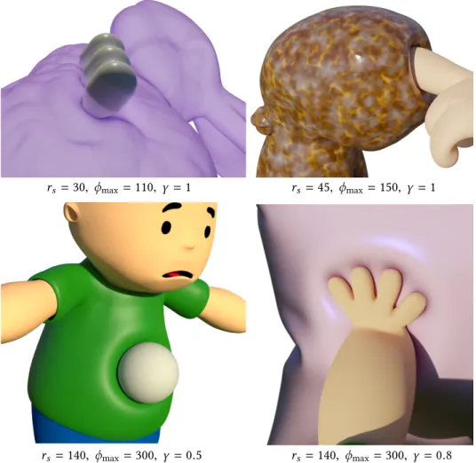
Figure 9 shows additional screenshots and the corresponding deformation parameters: a three-teeth comb sliding on an elastic Stanford bunny, a hard ball colliding with the soft character belly, and his hand plunging in a soft cushion and squishing a jellyfish-like octopus. In the bunny example, we have three different intersection zones, each of them contributing to the same deformable region.

rs = 140, ϕmax= 300, γ = 0.8 rs = 30, ϕmax= 110, γ = 1

rs = 140, ϕmax= 300, γ = 0.5

rs = 45, ϕmax= 150, γ = 1

Fig. 9. Four results of our deformer involving more complex objects (please also see the accompanying video).

In the pillow example, there is only one intersection zone, but multiple disconnected contact regions are merging and splitting during the animation. The video also shows an interactive session where the character pose is modified while the deformer is applied live, which is only made possible by the time-independency of our approach.

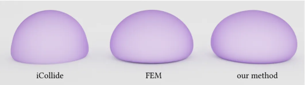
Comparisons.In Figure 10, we compare our method to a simulation based on finite elements in Houdini SideFX, and to the iCollide procedural deformer provided as a plugin for Autodesk Maya. In the case of the simulation, we have made an elastic sphere fall on a rigid plane until it bounces off it. We have then matched by hand the translation motion of the sphere so that its highest point is matched with the highest point in the simulation. The parameters of both iCollide and our deformer (constant throughout the animation) have finally been adjusted manually to visually match the result of the simulation. We provide simulation and deformer parameters in Appendix B.

As seen in the accompanying video where the comparison is shown in motion, our deformer is able to faithfully match the deformations and bulging effects observed in the simulation, whereas iCollide produces obviously different results.

FEM our method iCollide

Fig. 10. Comparison of deformers with simulation. Center: FEM simulation in Houdini©_{SideFX. Left:}

iCollide procedural deformer in Autodesk Maya©_{. Right: our method.}

5.2 Performance

Table 1 reports breakdown timings of our prototype implementation measured on a single core of an Intel i7-4790K CPU. On average they range from 6ms to 730ms depending on the working region complexity (Table 2). The size of the working region provides a tradeoff between quality of the deformation and performance. On the one hand, the larger this user-defined region is, the closer to a pseudo-geodesic distance the parametrization will be. On the other hand, the cost of the computations performed over this whole region (i.e., intersections and parametrization) will increase. For example on the comb-bunny test case, those two steps represent more than 75% of the computation time, since the deformable region only account for 12% of the working region vertices. Those numbers should be taken with care as our current implementation is non-optimized. For instance, we measured that the 5 linear solves involved in the “param” to “guides” steps represent only 50% of the computation time of those steps, whereas they are expected to completely dominate. Nonetheless, those results are very promising as we already achieve interactive performance for working regions up to 20k triangles.

Putting low-level implementation details aside, the major bottlenecks are expected to be the spatial searches of Section 3 (intersection, mapping, ball-testing/sliding), and the multiple sparse matrix factorizations. The formers are embarrassingly parallel and could thus greatly benefit from a multi-threaded or a GPU implementation. The intersection detection step itself could benefit from the collision detection literature [Ericson 2004; Teschner et al. 2005]. We also envision great optimization opportunities of the ball-sliding step (Section 3.3) by devising a dedicated AABB-tree traversal exploiting the fact that one of the ball extremities is empty since it was already accepted at the ball testing step.

Our approach involves 6 sparse linear solves at every frame, which currently requires 5 matrix factorizations because the different Poisson problems are carried out on slightly different domains while involving different least-squares linear constraints. Only the diffusion of the amplitude and slope fields shares the exact same matrix. Huge speedups could thus be achieved by pre-factorizing the standard Laplacian matrix over the whole region of interest of the elastic object only once, and then localize and adjust the problems through fast, structure-preserving, rank updates [Herholz and Alexa 2018]. Herholz et al. reported up to 10× speedups with such a technique.

6 DISCUSSIONS

Detailed surfaces.Throughout our pipeline, the elastic surface is assumed to be smooth. If that is not the case, the defacto standard solution is to encode the details within a displacement map on top of a smooth base surface. The details should then be re-introduced after the base-surface

Table 1. Runtime statistics for a pair of rigid and elastic meshes with a number of vertices (# vert) inside the deformable region D; average computation time over an animation broken down in terms of detecting the regions in intersection (i.) §3.1, building the mapping between them (m.) §3.2, extracting the contact zone (c.) §3.3, computing the deformation region parametrization (p.) §4.1, diffusing the directions of defor-mation (di.) §4.2 and the guiding fields (g.) §4.3, and deforming the surface according to the profile with γ = 1 (de.) §4.4, in percentage of the average total computation time (total).

scenes D relative time (%) total rigid elastic (# vert) i. m. c. p. di. g. de. time (ms)

caps caps 2608 19.3 4.4 15.4 22.0 19.0 7.8 12.1 50.8 caps v. caps 1120 20.8 2.7 14.4 23.4 14.8 9.0 14.9 18.9 caps caps 1913 16.7 1.3 9.4 32.4 14.3 9.0 16.8 29.7 v. caps caps 875 18.4 1.9 12.4 39.5 7.4 5.0 15.5 23.4 plane sphere 568 17.9 3.4 17.5 20.3 16.8 9.4 14.8 9.93 sphere plane 1456 12.5 2.2 15.6 21.6 17.7 11.6 18.7 16.9 s. sphere b. sphere 9995 4.1 0.6 21.0 26.5 25.4 13.7 8.7 233.1 window hand 1064 48.2 6.7 7.1 18.8 12.7 1.8 4.8 69.1 comb bunny 4413 10.1 0.6 8.5 65.2 4.1 1.9 9.7 378.4 finger squid 13144 4.6 0.5 10.2 53.5 19.2 5.7 6.4 646.8 ball torso 407 22.1 4.5 12.1 19.9 13.0 10.5 17.9 6.2 hand pillow 18612 5.2 0.8 32.0 31.2 19.4 5.0 6.3 728.5

Table 2. Number of vertices (# vert) inside the working region We_{of the meshes used in the test cases of}

Figures 1, 6 and 9.

mesh caps vertical caps plane sphere small sphere big sphere window hand # vert 3028 1465 1521 639 635 10183 22862 2314 mesh bunny comb squid finger torso ball hand pillow

# vert 35542 1831 29871 1209 529 521 2285 26234

deformation. To make the details vanish at the actual contact, displacement magnitudes should be scaled by a function proportional to our 1D parametrization u.

Region mapping.Our approach is sensitive to the quality of the mapping between the rigid and elastic surfaces (Section 3.2). If this mapping exhibits strong distortions and stretching, then the contact zone of the rigid surface might become under-sampled by the respective projected part of the elastic surface, thus leading to discretization artifacts (Figure 11). A practical solution is to refine the elastic mesh in this area. Ultimately, it would be interesting to devise an algorithm computing the mapped contact zones without a pre-established parametrization, such that the respective areas of these zones on both the rigid and elastic surfaces are the same. A perhaps less challenging research direction would be to investigate on-demand local parametrizations [Herholz and Alexa 2019] that could be computed in a such a way as to minimize stretching around the foreseen contact regions.

Time independence.We have argued throughout this paper that time-independence is key to enable non-linear editing of animations with efficient artistic control and deterministic re-sponses. However, some deformations such as those involving strong friction effects are inher-ently time-dependent. In a similar vein, our approach requires a surface-to-surface intersection

Fig. 11. Discretization issue. Left (clipped view): when the rigid sphere of Figure 6 plunges too deeply into the elastic one, the mapping between the two surfaces inevitably exhibits strong stretching (the undeformed sphere is visualized in purple). Right (side view): the amount of stretching is better seen after hiding the rigid small sphere.

between the two objects. If a tiny rigid object (in purple, with position at a previous frame in light-purple) entirely crosses the elastic surface (in grey), then we could not generate any deformation response. For such extreme penetrations, even a volumetric collision detection would not be sufficient to figure out in which direction the elastic object should be squashed. A practical workaround to this problem would be to let the artist design a proxy shape bounding the rigid surface (dashed lines), hence creating an intersection with the elastic surface at the desired location.

7 CONCLUSIONS

We have presented a deformation technique that works directly on two input surface meshes in a time-independent fashion to produce art-directable bulging effects. It presents several advantages in the context of animation pipelines: besides instant feedback and fine-tuning, it grants exploration over different combinations of character poses and bulging effects when objects come in contact. We deem our local surfacic approach as complementary to volumetric methods that work at coarser scales to deform an entire elastic object (i.e., [Aldrich et al. 2011]).

Our method opens the door to many future work directions ranging from speed improvements to the exploration of artistic control tools. A more general perspective would be to investigate the extension of our approach to the intersection of two elastic surfaces with possibly different pseudo-stiffness parameters. This would nicely complement geometric skinning with contact handling, bulging control, and other artistically-driven effects.

ACKNOWLEDGMENTS

We would like to thank the anonymous reviewers for their comments and advice. This work has been supported by the ANR Fold-Dyn project (ANR-16-CE33-0015). The 3D character Kaea Rig was created by Y4Lc1n (https://www.blendswap.com/blend/15982) and released under CC-BY-NC. The squid model Teodule is part of SOFA (https://www.sofa-framework.org/). The Stanford Bunny was originally 3D scanned by the Stanford Computer Graphics Laboratory.

REFERENCES

Nadine Abu Rumman and Marco Fratarcangeli. 2015. Position-Based Skinning for Soft Articulated Characters. Computer Graphics Forum34, 6 (2015), 240–250. https://doi.org/10.1111/cgf.12533

G. Aldrich, D. Pinskiy, B. Hamann, and Walt Disney Anim. Studios. 2011. Collision-Driven Volumetric Deformation on the GPU.. In Eurographics (Short Papers). 9–12.

Alexis Angelidis and Karan Singh. 2007. Kinodynamic Skinning Using Volume-preserving Deformations. In Proceedings of the 2007 ACM SIGGRAPH/Eurographics Symposium on Computer Animation (SCA ’07). Eurographics Association, 129–140. Jan Bender, Matthias Müller, and Miles Macklin. 2015. Position-Based Simulation Methods in Computer Graphics. In EG

2015 - Tutorials. https://doi.org/10.2312/egt.20151045

Mario Botsch and Leif Kobbelt. 2004. An Intuitive Framework for Real-time Freeform Modeling. ACM Trans. Graph. 23, 3 (2004), 630–634. https://doi.org/10.1145/1015706.1015772

Sofien Bouaziz, Sebastian Martin, Tiantian Liu, Ladislav Kavan, and Mark Pauly. 2014. Projective Dynamics: Fusing Constraint Projections for Fast Simulation. ACM Trans. Graph. 33, 4 (2014), 154:1–154:11. https://doi.org/10.1145/2601097.2601116 Keenan Crane, Clarisse Weischedel, and Max Wardetzky. 2013. Geodesics in Heat: A New Approach to Computing Distance

Based on Heat Flow. ACM Trans. Graph. 32, 5 (2013), 152:1–152:11.

Crispin Deul and Jan Bender. 2013. Physically-Based Character Skinning. In Virtual Reality Interactions and Physical Simulations (VRIPhys). Eurographics Association.

Herbert Edelsbrunner and Ernst P. Mücke. 1994. Three-dimensional Alpha Shapes. ACM Trans. Graph. 13, 1 (1994), 43–72. https://doi.org/10.1145/174462.156635

Christer Ericson. 2004. Real-Time Collision Detection. CRC Press, Inc.

Ming Gao, Nathan Mitchell, and Eftychios Sifakis. 2014. Steklov-Poincaré Skinning. In Proceedings of the ACM SIG-GRAPH/Eurographics Symposium on Computer Animation (SCA ’14). Eurographics Association, 139–148.

David Harmon, Daniele Panozzo, Olga Sorkine, and Denis Zorin. 2011. Interference-aware Geometric Modeling. ACM Trans. Graph.30, 6 (2011), 137:1–137:10. https://doi.org/10.1145/2070781.2024171

Philipp Herholz and Marc Alexa. 2018. Factor Once: Reusing Cholesky Factorizations on Sub-Meshes. ACM Transaction on Graphics37, 6 (2018). https://doi.org/10.1145/3272127.3275107

Philipp Herholz and Marc Alexa. 2019. Efficient Computation of Smoothed Exponential Maps. Computer Graphics Forum 38 (2019), 79–90. https://doi.org/10.1111/cgf.13607

Ladislav Kavan and Olga Sorkine. 2012. Elasticity-inspired Deformers for Character Articulation. ACM Trans. Graph. 31, 6 (2012), 196:1–196:8. https://doi.org/10.1145/2366145.2366215

Felix Knöppel, Keenan Crane, Ulrich Pinkall, and Peter Schröder. 2013. Globally Optimal Direction Fields. ACM Trans. Graph.32, 4 (2013), 59:1–59:10. https://doi.org/10.1145/2461912.2462005

Martin Komaritzan and Mario Botsch. 2018. Projective Skinning. Proc. ACM Comput. Graph. Interact. Tech. 1, 1 (2018), 12:1–12:19. https://doi.org/10.1145/3203203

John Lasseter. 1987. Principles of Traditional Animation Applied to 3D Computer Animation. SIGGRAPH Comput. Graph. 21, 4 (1987), 35–44. https://doi.org/10.1145/37402.37407

Bruno Lévy, Sylvain Petitjean, Nicolas Ray, and Jérome Maillot. 2002. Least Squares Conformal Maps for Automatic Texture Atlas Generation. ACM Trans. Graph. 21, 3 (2002), 362–371. https://doi.org/10.1145/566654.566590

J. P. Lewis, Matt Cordner, and Nickson Fong. 2000. Pose Space Deformation: A Unified Approach to Shape Interpolation and Skeleton-driven Deformation. In Proceedings of SIGGRAPH ’00. ACM, 165–172. https://doi.org/10.1145/344779.344862 Yijing Li and Jernej Barbič. 2019. Multi-Resolution Modeling of Shapes in Contact. Symposium on Computer Animation

(SCA), and Proc. of the ACM in Computer Graphics and Interactive Techniques (PACMCGIT)2, 2 (2019).

Ligang Liu, Lei Zhang, Yin Xu, Craig Gotsman, and Steven J. Gortler. 2008. A Local/Global Approach to Mesh Parameterization. In Proceedings of the Symposium on Geometry Processing (SGP ’08). Eurographics Association, 1495–1504. https: //doi.org/10.1111/j.1467-8659.2008.01290.x

Aleka McAdams, Yongning Zhu, Andrew Selle, Mark Empey, Rasmus Tamstorf, Joseph Teran, and Eftychios Sifakis. 2011. Efficient Elasticity for Character Skinning with Contact and Collisions. ACM Trans. Graph. 30, 4 (2011), 37:1–37:12. https://doi.org/10.1145/2010324.1964932

Andrew Nealen, Matthias Müller, Richard Keiser, Eddy Boxerman, and Mark Carlson. 2006. Physically Based Deformable Models in Computer Graphics. Computer Graphics Forum 25, 4 (2006), 809–836. https://doi.org/10.1111/j.1467-8659.2006. 01000.x

Jesús R Nieto and Antonio Susín. 2013. Cage based deformations: a survey. In Deformation models. Springer, 75–99. Damien Rohmer, Stefanie Hahmann, and Marie-Paule Cani. 2009. Exact Volume Preserving Skinning with Shape Control.

In Proceedings of the 2009 ACM SIGGRAPH/Eurographics Symposium on Computer Animation (SCA ’09). ACM, 83–92. https://doi.org/10.1145/1599470.1599481

Thomas W. Sederberg and Scott R. Parry. 1986. Free-form Deformation of Solid Geometric Models. SIGGRAPH Comput. Graph.20, 4 (1986), 151–160. https://doi.org/10.1145/15886.15903

Breannan Smith, Fernando de Goes, and Theodore Kim. 2018. Stable Neo-Hookean Flesh Simulation. ACM Trans. Graph. 37, 2 (2018), 12:1–12:15. https://doi.org/10.1145/3180491

Yun Teng, Miguel A. Otaduy, and Theodore Kim. 2014. Simulating Articulated Subspace Self-contact. ACM Trans. Graph. 33, 4 (2014), 106:1–106:9. https://doi.org/10.1145/2601097.2601181

M. Teschner, S. Kimmerle, B. Heidelberger, G. Zachmann, L. Raghupathi, A. Fuhrmann, M.-P. Cani, F. Faure, N. Magnenat-Thalmann, W. Strasser, and P. Volino. 2005. Collision Detection for Deformable Objects. Computer Graphics Forum 24, 1 (2005), 61–81. https://doi.org/10.1111/j.1467-8659.2005.00829.x

R. Vaillant, L. Barthe, G. Guennebaud, M.P. Cani, D. Rohmer, B. Wyvill, O. Gourmel, and M. Paulin. 2013. Implicit Skinning: Real-time Skin Deformation with Contact Modeling. ACM Trans. Graph. 32, 4 (2013), 125:1–125:12. https: //doi.org/10.1145/2461912.2461960

R. Vaillant, G. Guennebaud, L. Barthe, B. Wyvill, and M.P. Cani. 2014. Robust Iso-surface Tracking for Interactive Character Skinning. ACM Trans. Graph. 33, 6 (2014), 189:1–189:11. https://doi.org/10.1145/2661229.2661264

Wolfram von Funck, Holger Theisel, and Helmut Seidel. 2008. Volume-preserving Mesh Skinning. In VMV. Wei Wang. 2015. A Collision Deformer for Autodesk Maya. Master’s thesis. Texas A & M University.

Y. Wang, A. Jacobson, J. Barbič, and L. Kavan. 2015. Linear Subspace Design for Real-time Shape Deformation. ACM Trans. Graph.34, 4 (2015), 57:1–57:11. https://doi.org/10.1145/2766952

A SOLVING LAPLACE EQUATION WITH LINEAR CONSTRAINTS

Several steps of our pipeline boils down to the resolution of a Poisson equation of the form ∆f = 0 with a set of linear constraints of the form (1 − αij)fi+ αijfj = bij, αij ∈ [0, 1] defined on a subset of the edges ij. Since we discretize the Laplace equation on a triangular mesh equipped with linear elements, we cannot guarantee in general that both the linear constraints and Laplace equation can be satisfied exactly. In practice, we thus turn them into soft constraints by solving them in the least-squares sense. In matrix form, this yields:

(L + β C⊤C)v = β C⊤· b,

where L is the cotangent Laplacian matrix, C is the matrix holding the left-hand-side of the linear constraints, and β is a weight balancing the diffusion with boundary terms. Observing that the norm of the rows of L are expected to be roughly 10 times larger than the ones of C⊤_{C, and that L} is negative semi-definite, we set β = −102_{to give slightly more weights to the linear constraints.} B PARAMETERS USED FOR FIGURE 10

For the object in the middle, we used Houdini FEM solver on a sphere of radius 1 with default solver settings, and the following other parameters:

Tet embedding Physics

max tet scale: 0.06 stiffness multiplier: 1000 min triangle scale: 0.03125 damping ratio: 0.8 discretization max resolution: 1024 mass density: 1000

shape/volume stiffness: 100/642 friction: 0.1

For the object at left, we used the iCollide deformer of the iDeform plugin for Autodesk Maya with the following parameters:

Global parameters Bulge shape bulge: 10 max range: 10 radius: 50 intersection range: 5

For the object at right, we used our deformer with:

Global parameters Profile shape pseudo-stiffnessrs: 25 v2.x: 0.2

deformation extentϕmax: 60 v3.x: 0.77

bulgeγ = 0.5

C PSEUDO-CODE

Algorithm Part 1- Contact zone

Input: a rigid Wr and an elastic We open surface with a continuous parametrization Output: the deformed elastic surface positions p′

User parameters: pseudo-stiffness rs, deformation extent ϕmax, bulge γ , profile shape v2.x, v3.x

1: Intersection detection ▷ §3.1

2: Compute intersection points {qe, qr} ∈∂(Wr∩ We), with coordinates in 2D parametric space

3: Region mapping ▷ §3.2

4: Find affine transform A minimizing Ík∥ek∥2, with ek = qr_k−A qe_k

5: Compute deformation field g by harmonic diffusion of ek 6: for all elastic vertex i ∈ Wr ∩ We do

7: pi′←3D position of A qe_i + gi on the rigid mesh

8: end for

9: Contact zone extraction ▷ §3.3

10: for alli ∈ Wr ∩ We do ▷ Ball testing

11: ifno p′_j,i inside the ball with radius rs and center ci = p′_i+ rsn′_i then

12: C ← C ∪ {p_i′}

13: end if

14: end for

15: for alledge ij with i ∈ C, and j < C do ▷ Ball sliding

16: Find smallest α such as p′_{− ((1 − α) ci+ α cj)} 2 −r_s2= 0 17: ∂C ← ∂C ∪ {(1 − α) p′ i + α p′j} 18: end for 19: ▷ continues in Part 2

Algorithm Part 2- Deformation

20: Deformable region parametrization ▷ §4.1

21: Solve ∆v = 0 in the least-squares sense with the linear constraints: ▷ App. A ▷ vi ←0 , ∀i ∈ ∂We

▷ (1 − αij)vi + αijvj = 1 , ∀ij crossing ∂C

22: Compute normalized gradients X = −∇v/∥∇v∥

23: Solve Poisson equation ∆ϕ = ∇ · X ensuring ϕ = 0 on ∂C 24: u ← ϕ/ϕmax

25: D ← {i ∈ We |ui ∈]0, 1]}

26: Direction field computation ▷ §4.2

27: for alledge ij ∈ D do

28: ¯Ri(j ←B⊤_i Ri₍jBj

29: end for

30: Interpolate ¯d over D by harmonic diffusion and parallel transport ▷ App. A

using ¯Ri(j and the linear least-squares constraints: ▷ ¯di = B⊤i ni, ∀i ∈ ∂D

▷ (1 − αij) ¯di+ αij¯dj = Bi⊤(pij− pij′)/∥pij− p′ij∥, ∀ edge ij crossing ∂C

31: for alli ∈ D do

32: di ←Bi ¯di +p1 − ∥¯di∥2ni

33: end for

34: Amplitude and slope fields computation ▷ §4.3

35: Interpolate a over D by harmonic diffusion with standard Dirichlet conditions:

▷ aj = Íi ∈Njαijaij/

Í

i ∈Njαij, ∀ edge ij crossing ∂C

▷ ak = mean(aj), ∀k ∈ ∂D

36: for alledge ij crossing ∂C do

37: ˜pij← pij+ ajdij

38: Find sijsuch as (pj + (−aj+ ujsij) dj−˜pij)⊤n_ij′ = 0

39: end for

40: Interpolate s over D by harmonic diffusion with standard Dirichlet conditions:

▷ sj = Íi ∈Njαijsij/

Í

i ∈Njαij, ∀ edge ij crossing ∂C

▷ sk = mean(sj), ∀k ∈ ∂D

41: Profile curves instantiation ▷ §4.4

42: Compute hvsuch as Íi ∈CAi ∥p′

i − pi∥= Íj ∈DAjHaj,sj(uj) ▷ pseudo-volume 43: for alli ∈ D do 44: θi ←tan-1(si/ai) 45: v₀← (0, −ai) 46: v₁← (0.2 cosθi, a_i(0.2 sinθi −1)) 47: v2← (1/3,γ · hv)

48: p′_i ← pi+ f2(f₁-1(ui)) di, with f1, f2defined using vk ▷ displacement

49: end for