LLR Computation for Multistage Decoding

HAL Id: hal-01576137

https://hal.archives-ouvertes.fr/hal-01576137

Submitted on 22 Aug 2017

HAL is a multi-disciplinary open access

archive for the deposit and dissemination of

sci-entific research documents, whether they are

pub-lished or not. The documents may come from

teaching and research institutions in France or

abroad, or from public or private research centers.

L’archive ouverte pluridisciplinaire HAL, est

destinée au dépôt et à la diffusion de documents

scientifiques de niveau recherche, publiés ou non,

émanant des établissements d’enseignement et de

recherche français ou étrangers, des laboratoires

publics ou privés.

LLR Computation for Multistage Decoding

Abir Ben Hadj Fredj, Jean-Claude Belfiore

To cite this version:

Abir Ben Hadj Fredj, Jean-Claude Belfiore. LLR Computation for Multistage Decoding. European

Conference on Networks and Communications (EuCNC 2016), Jun 2016, Athènes, Greece.

�hal-01576137�

LLR Computation for Multistage Decoding

Abir Ben Hadj Fredj

Telecom ParisTech Paris, France abir.benhadjfredj@telecom-paristech.fr

Jean-Claude Belfiore

Abstract—Due to their linear and highly symmetrical struc-ture, lattices are becoming of a great interest as potential transmission schemes. Lattice codes suggest a common view of channel and source coding and new tools for the analysis of information network problems. Several constructions have been proposed to build these lattices, some of which are based on multi-level coding and multistage decoding such as constructions D and πD. Soft-decision decoders corresponding to the different

nested error-correcting codes used to construct such lattices need at each stage the computation of a soft input, namely Log-Likelihood Ratios. In this paper, we give an efficient computation of LLRs based on Jacobi theta functions for three different types of constructions; Binary construction D, Quaternary construction D and Binary construction πD.

I. INTRODUCTION

In Gaussian multiple access channels (MAC), where two or more users transmit information to the same receiver over a gaussian channel, interference has always been considered as nuisance. Several methods have been developed to avoid interference in MAC such as orthogonal access to the channel techniques (FDMA,TDMA..). However, avoiding interference may impact data rates as they decrease when the network size increases. Physical-layer network coding introduced in 2006 by Zhang et al. in [1], comes up with a revolutional concept allowing to harness interference instead of avoiding it. Based on this new concept, B. Nazer and M. Gastpar in [2], proposed a new strategy, Compute and Forward, that enables relays to decode linear equations of the transmitted messages using the noisy linear combinations provided by the channel. In order to be decoded reliably, the messages must be lattice points whose algebraic structure enables that integer linear combinations of these points remain a lattice point. Several binary and M-ary lattice constructions have been proposed to construct lattices such as construction A and other equivalent constructions namely B, D, πAand πD.

One of the main drawbacks of construction A is that in order to be good for AWGN channel, the underlying linear codes have to be implemented over very large prime fields which in turn result in high decoding complexity. Constructions D and πD which are based on multi-level coding guarantee a

low-complexity encoding scheme as well as a practical decoding based on multistage decoding. Different error-correcting codes are used in these lattice constructions. For construction D and for construction πD, one must have respectively a family of

nested codes and a family of equivalent codes. At the receiver side, in order to decode one lattice point, we must decode

all the codewords corresponding to the different used error-correcting codes. In the binary case, Log-Likelihood Ratios (LLRs) which are the inputs for the soft-decoding algorithms must be calculated at each stage of the multistage lattice decoder. LLR = logP(y 0 ij|xij = 0) P(y0ij|xij = 1) (1)

where y0_ij and xij are respectively the jth received bit after

the modulo operation and the jth _{transmitted bit at the i}th

level of the multistage decoder. For Compute and Forward, decoding is performed over the whole lattice, therefore LLRs are computed over the whole lattice which induce an infinite sum of exponentials. Thus, the computations of exact LLRs are very complex for a practical implementation.

In this paper, we propose an LLR computation for gaussian channels based on Jacobi theta functions. To calculate LLRs, we only need to know the value of two types of theta functions. These values can be precalculated easily and stored in lookup tables.

This paper is organized as follows; In the second section, we give some basic definitions on lattices and different construc-tions as well as the system model. We will also provide some fundamental computation rules of theta functions that we will exploit to perform our calculations. In section three, we will deal with the Gaussian channels and give our LLR expressions as functions of Jacobi theta functions for three different lattice constructions.

Throughout this paper, vectors and matrices are denoted by lowercase and uppercase bold letters, such as a and A, respectively. The probability of a given event E is denoted by P(E).

II. PRELIMINARIES AND SYSTEM MODEL

An n−dimensional euclidean lattice Λ is an additive dis-crete subgroup of Rn. Roughly speaking, a lattice is a periodic arrangement of points in the n−dimensional Euclidean space [3]. The fundamental Voronoi region, RΛ, of a lattice Λ, is the

set of all points in Rn_{that are closest to the zero vector. A pair}

of euclidean lattices (Λ1, Λ2) is nested if Λ2 ⊆ Λ1, and the

finite quotient group Λ1/Λ2 is called a lattice partition whith

index |Λ1/Λ2|. The partition index is the number of cosets

partition chain Λ1/Λ2/.../Λr.

Multi-level coding is a practical encoding scheme for lattices. It uses several error-correcting codes and the transmitted symbols are constructed by combining symbols of codewords of these codes [4]. It has been proved in [5] that multi-level coding (MLC) and multistage decoding (MSD)[6] suffice to approach capacity if the rates at each level are appropriately chosen. Construction D is based on this multi-level nature. As an example, let us consider the lattice partition chain Zn/2Zn/4Zn/..../2rZn and the linear binary code Ci(n, ki),

the code associated to the partition 2i

Zn/2i+1Zn. We consider as well a family of r nested codes C0 ⊆ C1⊆ ... ⊆ Cr−1.

Then the lattice Λ can be defined as follows:

Λ1= 2rZn+ 2r−1Cr−1(n, kr−1) + ... + C0(n, k0) (2)

On the receiver side, a practical decoding algorithm is used, known as multistage decoding. The idea behind is that every code is decoded individually, in other words, we decode C0,

and then based on the estimated codeword we decode C1and

so forth, until we have decoded all the codewords. To decode code Ci, we implement a soft-decision decoding algorithm,

therefore, at each stage we need to calculate a soft-input which is the Log-Likelihood Ratio. However, LLR computations induce infinite sums of exponentials. It is then time and energy consuming [7]. In this paper, we deal with several lattice constructions each corrresponding to different lattice partition chain. The choice of such construction is related to ideals and their factorization; Hereinafter, we consider fields of characteristic 2. For example F2, F4,F8. We also consider

lattices based on complex constellations Z[β] where β is a complex root of a quadratic polynomial with coefficients in Z.

The choice of the construction is based on the prime factor-ization of the principal ideal generated by 2; we have three different cases:

• _{2 ramifies in Z[β],so we have 2Z[β] = I}2, where I is the prime ideal: Binary construction D

• 2 remains inert over Z[β], so we have 2Z[β] is a prime

over Z[β]: Quaternary construction D

• 2 splits into two distinct prime ideals over Z[β], so we

have 2Z[β] = I · ¯I: Binary construction πD

For each of these three cases, we consider one example:

• 2 ramifies: β = i • 2 is inert: β = ω = −1+i √ 3 2 • 2 splits: β = 1+ √ −7 2

The prime ideals resulting from the factorization of 2 have a lattice structure and are in fact sublattices of Λ1, let’s call

them Λ2

1) System Model: The n−dimensional lattice point x is sent through an AWGN channel giving the received point y = x + w, where w is a length-n vector of zero-mean σ2

-variance gaussian distributed independant random variables. We consider a constellation carved out from a lattice Λ1 and

we consider the lattice partition Λ1/Λ2. A multistage decoding

algorithm was introduced in [8] and [9] which feeds soft values of the received observation y into the binary decoder at each level. Each level of the construction D may be viewed as construction A. We consider the previous example (2) and the received signal y = x+w so MSD can be described as follows:

• First y is reduced to y0₁≡ y mod 2, only the codeword

corresponding to the code of the smallest rate remains.

• The soft-inputs to the decoder are then calculated based

on the value of y0₁. Based on these values, the decoder of the code C0 finds a decoded codeword ˆc0. The estimated

codeword is then substracted from y to give ˜y = y − ˆc0 • The next step will be to divide ˜y by 2, the modulo

operation is again performed to get ˜y0₂ and the LLRs are calculated based on the values of ˜y02

• All the steps listed above are repeated until we get all the estimated codewords that correspond to the nested codes Ci

• _{Finally, only the element of Z}n that we call b remains. Then a decoder for Zn _{finds a sequence ˆb and we get the}

estimated lattice point ˆy

So as we can see, due to the structure of the multistage decoder, the received signal is, at each level, subject to a modulo 2 operation. The resulting signal can be written as follows:

y0= y mod 2 = x mod 2 + w mod 2 = c0+ w0 (3)

It follows from (3) that c0 ∈ C0. The modulo 2 operation

folds up the Gaussian Noise resulting in a vector w0distributed according to the Wrapped Normal distribution [10]. Its prob-ability density function (PDF) fσ2(w0). Let g_σ2(w) be the

probability density function of the Gaussian noise w ∈ Rn_.

gσ2(w) and f_σ2(w0) can be written as follows:

gσ2(w) = (2πσ2) −n 2 _e −kwk2 2σ2 (4) fσ2(w0) = X b∈2Zn gσ2(w0+ b) (5)

w0 lives in the fundamental Voronoi region of 2Zn that we call RV(2Zn).

To decode ci we use a soft-decision decoder, consequently

we must at each stage calculate the decoder soft-inputs which are Log-Likelihood Ratios. The caculations are very complex especially when we have several levels. Thus to simplify the multistage decoding algorithm, we propose an efficient computation of LLRs based only on Jacobi theta functions. In the non-binary case LLR vectors will be defined.

2) Jacobi Theta Functions: To each lattice Λ we can associate a Jacobi theta function ΘΛ. Jacobi theta functions are

the elliptic analogues of the exponential functions. There are several closely related functions called Jacobi theta functions, and many different and incompatible systems of notation for them. One Jacobi theta function defined as a function of two variables u and τ , where u is a complex number and τ is defined in the upper half plane.

ΘΛ(u, q) = ∞

X

n=−∞

qn2e2inu (6) where q = eiπτ. There are four different types of elementary Jacobi theta functions. Hereinafter, we will be interested in ϑ2

and ϑ3. Note that these two types are even functions of the

variable u ϑ3(u, q) = ∞ X k=−∞ qk2e2iku (7) ϑ2(u, q) = ∞ X k=−∞ q(k+12) 2 e(2k+1)iu (8)

3) Computation rules of theta functions: Here we introduce some fundamental Jacobi theta functions’computation rules that we will exploit later for the calculation of the different LLRs.

• Scaling: ΘαΛ1(u, q) = ΘΛ1(αu, q

α2

) ; α > 0

• Direct Sum: ΘΛ1⊕Λ2(u, q) = ΘΛ1(u1, q)ΘΛ2(u2, q)

u = (u1, u2)

• Union: ΘΛ1∪Λ2(u, q) = ΘΛ1(u, q) + ΘΛ2(u, q)

III. EFFICIENTLLRCOMPUTATION BASED ONJACOBI

THETA FUNCTIONS FORGAUSSIANCHANNELS

A. Binary Construction D

1) Real Case: In this section, we consider the one-dimensional partition chain Z/2Z/4Z.../2rZ. As we can see, the quotient ring Z/2Z has index 2, and Z is the disjoint union of two cosets 2Z and 2Z + 1. We define the set of coset representatives as A = {0, 1}. Here, Log-Likelihood Ratios are defined as follows:

LLR = logP(y

0

ij|xij= 0)

P(yij0 |xij= 1)

(9)

The theta functions of Z and Z + 12 can be written in terms

of ϑ3 and ϑ2. Known that ϑ2 can also be written in terms of

ϑ3, all the given results can be reduced to functions of ϑ3.

Θ_Z(y, σ2) =X x∈Z e2i2σ2iy xe −x2 2σ2 = ϑ3( iy 2σ2, e −1 2σ2) (10) Θ_Z+1 2(y, σ 2 ) =X x∈Z e2i2σ2iy (2x+1)e −(x+ 1 2)2 2σ2 = ϑ2( iy 2σ2, e −1 2σ2) (11)

Now, using the computation rules given above, we have the following results for the cosets 2Z and 2Z + 1:

-4 -2 2 4

-4 -2 2 4

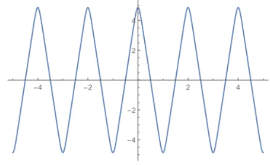
Fig. 1. LLRs for the binary real construction D for σ = 0.2db

Θ_2Z(y, σ2) =X x∈Z e2iσ2iyxe −2x2 σ2 (12) Θ_2Z+1(y, σ2) =X x∈Z e2iσ2iy(2x+1)e −2(x+ 1₂)2 σ2 (13)

Then Log-Likelihood Ratios can be defined as follows:

P(y|x = 0) = √1 2πσ X k∈Z e−ky−2kk22σ2 =e −kyk2 2σ2 √ 2πσ X k∈Z e2ykσ2 e −2k2 σ2 =e −kyk2 2σ2 √ 2πσϑ3( iy σ2, e −2 σ2) (14) P(y|x = 1) = X k∈Z e−ky−(2k+1)k22σ2 = e −kyk2 2σ2 √ 2πσ X k∈Z ey(2k+1)σ2 e −2(k+ 1 2)2 σ2 = e −kyk2 2σ2 √ 2πσϑ2( iy σ2, e −2 σ2) (15) LLR = logP(y|x = 0) P(y|x = 1) = logϑ3( iy σ2, e −2 σ2) ϑ2(_σiy2, e −2 σ2) (16)

LLRs in the case of a real binary construction D are shown in figure 1.

2) Complex Case: (2 ramifies): Complex binary construc-tion D is also another way to construct lattices. In this case, we consider the two-dimensional lattice partition chain Z[i]/(1 + i)Z[i]/2Z[i]..., where Z[i] is the ring of Gaussian integers. As in the real case the set of coset representatives is defined this way A = {0, 1}.

Known that, Z[i]/(1 + i)Z[i] is equivalent to Z2/D2where

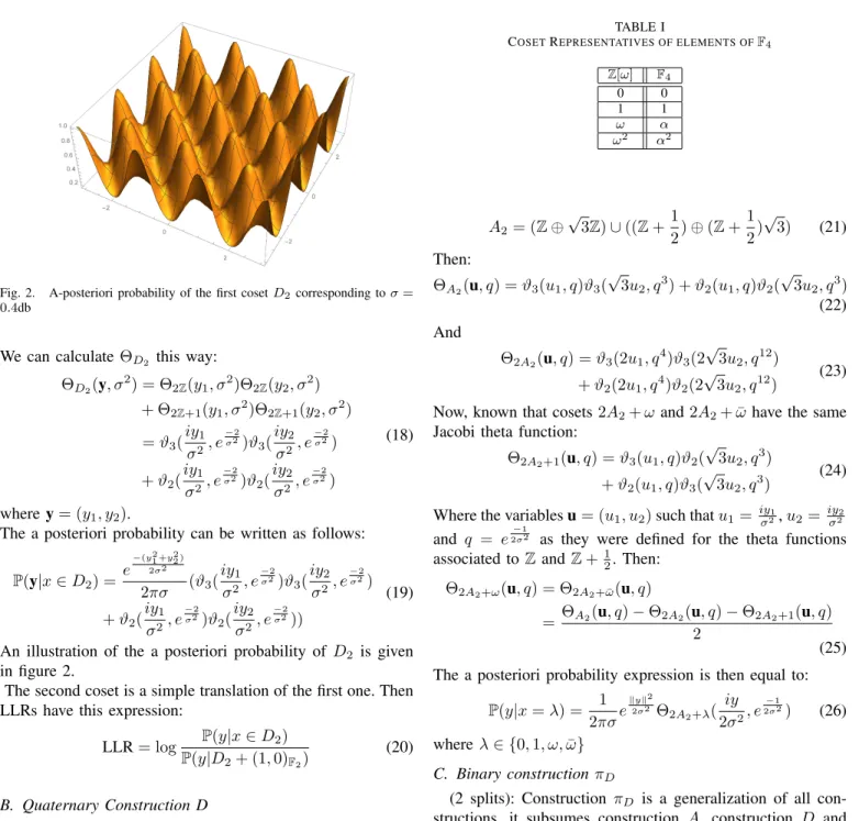
Fig. 2. A-posteriori probability of the first coset D2 corresponding to σ =

0.4db

We can calculate ΘD2 this way:

ΘD2(y, σ 2_{) = Θ} 2Z(y1, σ2)Θ2Z(y2, σ2) + Θ_2Z+1(y1, σ2)Θ2Z+1(y2, σ2) = ϑ3( iy1 σ2, e −2 σ2)ϑ₃(iy2 σ2, e −2 σ2) + ϑ2( iy1 σ2, e −2 σ2)ϑ₂(iy2 σ2, e −2 σ2) (18) where y = (y1, y2).

The a posteriori probability can be written as follows:

P(y|x ∈ D2) = e −(y2_{1 +y}2 2 ) 2σ2 2πσ (ϑ3( iy1 σ2, e −2 σ2)ϑ₃( iy2 σ2, e −2 σ2) + ϑ2( iy1 σ2, e −2 σ2)ϑ₂(iy2 σ2, e −2 σ2)) (19)

An illustration of the a posteriori probability of D2 is given

in figure 2.

The second coset is a simple translation of the first one. Then LLRs have this expression:

LLR = log P(y|x ∈ D2) P(y|D2+ (1, 0)F2)

(20)

B. Quaternary Construction D

(2 is inert): By choosing a bigger alphabet size, one can increase coding gain. Quaternary contruction D is based on partition chains of the densest lattice in dimension 2 which is the hexagonal lattice A2. Here we consider the

two-dimensional, four-way partition Z[ω]/2Z[ω]/4Z[ω].., where ω = e2iπ3 . Z[ω] is called the ring of the Eisenstein integers.

Log-Likelihood Ratios can be defined as length-three vectors normalized with respect to P(y|x = 0):

LLR =     logP(y|x=1) P(y|x=0) logP(y|x=α) P(y|x=0) logP(y|x=α2) P(y|x=0)    

Here, the partition index is |Z[ω]/2Z[ω]| = 4 and the quotient ring Z[ω]/2Z[ω] is isomomorphic to F4(see Table I)

We consider Z[ω]/2Z[ω] which is equivalent to Z2_/2A 2.

TABLE I

COSETREPRESENTATIVES OF ELEMENTS OFF4

Z[ω] F4 0 0 1 1 ω α ω2 α2 A2= (Z ⊕ √ 3Z) ∪ ((Z +1₂) ⊕ (Z +1₂)√3) (21) Then: ΘA2(u, q) = ϑ3(u1, q)ϑ3( √ 3u2, q3) + ϑ2(u1, q)ϑ2( √ 3u2, q3) (22) And Θ2A2(u, q) = ϑ3(2u1, q 4 )ϑ3(2 √ 3u2, q12) + ϑ2(2u1, q4)ϑ2(2 √ 3u2, q12) (23) Now, known that cosets 2A2+ ω and 2A2+ ¯ω have the same

Jacobi theta function:

Θ2A2+1(u, q) = ϑ3(u1, q)ϑ2( √ 3u2, q3) + ϑ2(u1, q)ϑ3( √ 3u2, q3) (24)

Where the variables u = (u1, u2) such that u1=iy_σ21, u2= iy_σ22

and q = e2σ2−1 as they were defined for the theta functions

associated to Z and Z +12. Then:

Θ2A2+ω(u, q) = Θ2A2+ ¯ω(u, q)

= ΘA2(u, q) − Θ2A2(u, q) − Θ2A2+1(u, q)

2

(25) The a posteriori probability expression is then equal to:

P(y|x = λ) = 1 2πσe kyk2 2σ2Θ_2A 2+λ( iy 2σ2, e −1 2σ2) (26) where λ ∈ {0, 1, ω, ¯ω} C. Binary constructionπD

(2 splits): Construction πD is a generalization of all

con-structions, it subsumes construction A, construction D and construction πA. It has been introduced in [11]. As for

con-struction D, this concon-struction is based on multivel coding and multistage decoding thus LLR calculations are needed at each stage. The decoding algorithm is very close to the decoding algorithm of construction D, however, in this case we have two lattice partition chains; Z[α]/I/2Z[α] and Z[α]/ ¯I/2Z[α], where α = 1+

√ −7

2 and we have a family of nested equivalent

codes. Coset representatives will be here couples (a1, a2) in

F2× F2(see table II).

Z[α] can be written as the product of an ideal I and its conjugate ¯_{I, 2Z[α] = I ¯}I

The lattice Z[α] can be defined as follows:

Z[α] = (Z ⊕ √

7Z) ∪ ((Z + 1₂) ⊕√_{7(Z +}1

LLR = log " ϑ3(iy_σ21, e −2 σ2)ϑ₃(iy2 σ2, e −2 σ2) + ϑ₂(iy1 σ2, e −2 σ2)ϑ₂(iy2 σ2, e −2 σ2) ϑ3(iy_σ21, e −2 σ2)ϑ₂(iy2 σ2, e −2 σ2) + ϑ₂(iy1 σ2, e −2 σ2)ϑ₃(iy2 σ2, e −2 σ2) # (20) TABLE II

COSETREPRESENTATIVES OF ELEMENTS OFF2× F2

Z[α] F2× F2 0 (0,0) 1 (1,1) α (0,1) ¯ α (1,0)

The Jacobi theta function associated to this lattice is: Θ_Z[α](y, σ2) = ϑ3( iy1 2σ2, e −1 2σ2)ϑ₃( √ 7iy2 2σ2 , e −7 2σ2) + ϑ2( iy1 2σ2, e −1 2σ2)ϑ₂( √ 7iy2 2σ2 , e −7 2σ2) (28)

where y = (y1, y2). Now, Z[α] can be written as the union of

four disjoint cosets:

Z[α] = 2Z[α] ∪ (2Z[α] + 1) ∪ (2Z[α] + α) ∪ (2Z[α] + ¯α) (29) (2Z[α] + α) and (2Z[α] + ¯α) have the same theta function: Θ_Z[α](u, q) = Θ_2Z[α](u, q)+Θ_2Z[α]+1(u, q)+2Θ_2Z[α]+α(u, q)

(30) On the other hand, we have:

Θ_2Z[α](y, σ2) = ϑ3( 2iy1 2σ2, e −2 σ2)ϑ₃(2 √ 7iy2 2σ2 , e −14 σ2 ) + ϑ2( 2iy1 2σ2, e −2 σ2)ϑ₂( 2√7iy2 2σ2 , e −14 σ2 ) (31) Θ_2Z[α]+1(y, σ2) = ϑ3( 2iy1 2σ2, e −2 σ2)ϑ₂( 2√7iy2 2σ2 , e −14 σ2 ) + ϑ2( 2iy1 2σ2, e −2 σ2)ϑ₃(2 √ 7iy2 2σ2 , e −14 σ2 ) (32) where y = (y1, y2). Then: Θ_2Z[α]+α(u, q) = Θ_{2Z[α]+ ¯}α(u, q)

= ΘZ[α](u, q) − Θ2Z[α](u, q) − Θ2Z[α]+1(u, q) 2

(33)

IV. CONCLUSION

We showed in this paper that the knowledge of the value of two types of Jacobi theta functions ϑ3 and ϑ2 is sufficient

for computing LLRs when constructions D or πD are used

to construct high dimensional lattice codes. Known that ϑ2

can be expressed in terms of ϑ3, the expressions of LLRs can

even be simpler. The calculation of Log-Likelihhod Ratios is then simplified; instead of having to calculate infinite sums of exponentials, one can have simple look-up tables containing values of Jacobi theta function ϑ3.

REFERENCES

[1] S Zhang SC Liew and P P Lam, Hot-topic Physical layer network coding. in Proc, 12th MobiCom, pages 358-365, New York, NY, USA 2006.

[2] B. Nazer and M. Gastpar. Compute-and-forward: Harnessing interference through structured codes. Information theory,IEEE transactions,vol.57,pp.6463-6486 Oct2011.

[3] J. Conway and N.J..A Sloane, sphere Packings, Lattices and groups.. Springer New York,2010

[4] H. Imai and S. Hirakawa A New multiLevel coding method using error-correcting codes. Information Theory, IEEE Transactionson, vol.23,pp 371-377, May 1977

[5] G. Forney, M. Trott, and S.,-Y. Chung Sphere-bound achieving coset codes and multilevel coset codes. Information Theory, IEEE Transac-tionson, vol.46,pp 820-850, May 2000

[6] G.D. Forney Jr., A bounded-distance decoding algorithm for the leech lattice, with generalizations. IEEE trans. Inf. Theory,vol.35,pp 906-909, July 1989

[7] Guido Montorsi and Farbod Kayhan Analog Digital Belief Propagation and its application to multi stage decoding systems. In Communications and Networking (BlackSeaCom), 2015 IEEE International Black Sea Conference on (pp. 82-86). IEEE May 2015

[8] A. Sakzad, M.-R. Sadeghi and D. Panario Construction of turbo lattices. In Allerton Conference on Communication,Control, and computing, 2010,Allerton,IL, pp. 14-21 Sept29-Oct1 2010

[9] K. Mardia, Statistics of Directional Data. Academic Press, 1972 [10] Yuh-Chih Huang and Krishna R. Narayanan Construction πAandπD

Lattices: Construction, Goodness, and decoding algorithms. Interna-tional Symposium on Information Theory 2014