Synchronization, stochasticity and phase waves in neuronal networks with spatially-structured connectivity

HAL Id: hal-03028996

https://hal.archives-ouvertes.fr/hal-03028996

Preprint submitted on 4 Jan 2021

HAL is a multi-disciplinary open access

archive for the deposit and dissemination of

sci-entific research documents, whether they are

pub-lished or not. The documents may come from

teaching and research institutions in France or

abroad, or from public or private research centers.

L’archive ouverte pluridisciplinaire HAL, est

destinée au dépôt et à la diffusion de documents

scientifiques de niveau recherche, publiés ou non,

émanant des établissements d’enseignement et de

recherche français ou étrangers, des laboratoires

publics ou privés.

Synchronization, stochasticity and phase waves in

neuronal networks with spatially-structured connectivity

Anirudh Kulkarni, Jonas Ranft, Vincent Hakim

To cite this version:

Anirudh Kulkarni, Jonas Ranft, Vincent Hakim. Synchronization, stochasticity and phase waves in

neuronal networks with spatially-structured connectivity. 2020. �hal-03028996�

Synchronization, stochasticity and phase waves

in neuronal networks with spatially-structured

connectivity

Anirudh Kulkarni1,2,3Y_{, Jonas Ranft}1,2YB_{, Vincent Hakim}1B_.

1 Laboratoire de Physique de l’Ecole Normale Sup´erieure, CNRS, Ecole Normale Sup´erieure, PSL University, Sorbonne Universit´e, Universit´e Paris-Diderot, Paris, France 2 IBENS, Ecole Normale Sup´erieure, PSL University, CNRS, INSERM, Paris, France 3 Present address: Department of Bioengineering, Imperial College London, London, United Kingdom

Y These authors contributed equally to this work. B jonas.ranft@ens.fr or vincent.hakim@ens.fr Version: June 4, 2020

Abstract

Oscillations in the beta/low gamma range (10-45 Hz) are recorded in diverse neural structures. They have successfully been modeled as sparsely synchronized oscillations arising from reciprocal interactions between randomly connected excitatory (E) pyramidal cells and local interneurons (I). The synchronization of spatially distant oscillatory spiking E-I modules has been well studied in the rate model framework but less so for modules of spiking neurons. Here, we first show that previously proposed modifications of rate models provide a quantitative description of spiking E-I modules of Exponential Integrate-and-Fire (EIF) neurons. This allows us to analyze the dynamical regimes of sparsely synchronized oscillatory E-I modules connected by long-range excitatory interactions, for two modules, as well as for a chain of such modules. For modules with a large number of neurons (> 105), we obtain results similar to previous obtained ones based on the classic deterministic Wilson-Cowan rate model, with the added bonus that the results quantitatively describe simulations of spiking EIF neurons. However, for modules with a moderate (∼ 104_{) number of neurons, stochastic variations in the spike}

emission of neurons are important and need to be taken into account. On the one hand, they modify the oscillations in a way that tends to promote synchronization between different modules. On the other hand, independent fluctuations on different modules tend to disrupt synchronization. The correlations between distant oscillatory modules can be described by stochastic equations for the oscillator phases that have been intensely studied in other contexts. On shorter distances, we develop a description that also takes into account amplitude modes and that quantitatively accounts for our simulation data. Stochastic dephasing of neighboring modules produces transient phase gradients and the transient appearance of phase waves. We propose that these stochastically-induced phase waves provide an explanative framework for the observations of traveling waves in the cortex during beta oscillations.

Introduction

Rhythms and collective oscillations at different frequencies are ubiquitous in neural structures [1]. Numerous works have been devoted to understanding their origins and

characteristics [2] which depend both on the neural area and on the activity of the animal. Gamma band oscillations (30-100 Hz) are for instance recorded in the visual cortex as well as several other structures and have been hypothesized to support various functional roles [3]. Beta oscillations (10-30 Hz) are prominent in the motor cortex during movement planning before movement initiation [4] and have traditionally been assigned a role in movement control while more general roles have also been proposed [5].

Several experimental results point out the need to model and analyze the spatial organization of oscillatory activity [6]. An early study [7], using widefield imaging and voltage-sensitive dyes, reported that stimulus-induced oscillatory activity around 10 Hz and 20 Hz was organized in plane waves and spiral waves in the turtle cortex. This spiral-like organization was also reported for pharmacologically induced 10 Hz oscillations in the rat visual cortex [8]. The underlying mechanisms and specific cells involved in the synchronization of two distant regions have more recently started to be investigated using optogenetic manipulations in mice [9].

A motivating illustrative example for the present theoretical study is the observation that beta oscillatory activity during movement preparation exhibits transient episodes of propagating waves in the motor cortex of monkeys [10–13] and humans [14]. These waves appear to propagate along particular anatomical directions with a typical wavelength of 1 cm and a velocity of about 20 cm · s−1[10]. On the structural side, the characterization of the long-range intracortical connectivity in motor cortex have given rise to several quantification endeavors in both monkeys [15, 16] and cats [17] with the strength of excitatory responses to microstimulation decaying on a 2 mm length scale. Can one connect these different observations in some ways and how? What is the proper mechanistic interpretation of these observed waves?

The study of waves in oscillatory media has been largely based on the analysis of oscillator synchronisation which itself has a long history [18]. Classic mathematical methods for studying synchronization of weakly coupled oscillators have been extended to study oscillations and travelling waves in spatially extended media in physics and chemistry [19]. In simple descriptions of neural network dynamics based on rate models introduced by Wilson and Cowan [20], also called neural-mass models, the dynamics of a whole set of neurons is reduced to a small set of differential equations approximately describing the temporal evolution of the firing rate of a “typical ”’neuron in the set. This allows one to directly apply the techniques developed to analyze synchronization of oscillators to study the synchronization properties of sets of oscillating neurons in the rate-model framework. This approach has been followed in a number of works to study the synchronization of spatially-coupled neural networks in the oscillatory regime [21–25]. Rate models with spatially-structured connectivity have also been extensively studied to analyze pattern formation in a neural network context since Amari’s work [26] (see [27–29] for reviews). A limitation is that rate models are generally difficult to quantitatively relate to models of single neurons.

Networks of model spiking neurons provide a more detailed description of neuronal network dynamics than rate models. Studies of networks with random unstructured connectivities have shown the existence of a “sparsely synchronized” oscillatory (SSO) regime [30] in which a collective oscillation exists at the whole population level while spike emission by single neurons is quite stochastic with no significant periodic component. Experimental recordings suggest that neural rhythms in the beta, gamma and higher frequency ranges operate in this regime [2]. Specifically, rhythms in the beta/low gamma range are thought to arise from sparse synchronization between excitatory (E) and inhibitory (I) neuronal populations with reciprocal interactions [31, 32], the so-called Pyramidal-Interneuron Gamma (PING) mechanism [33].

A few studies have considered the impact of structured connectivity on sparsely synchronized oscillations in the spiking-network framework. The influence of delays

in synaptic transmission was studied in [34] for the synchronization of two neuronal E-I modules oscillating in the high-gamma frequency range, using a classic rate-model formalism. A variety of dynamical regimes was found and qualitative agreement with the bifurcations observed in simulations of a spiking network was reported when the neurons in each E-I module oscillated in a well-synchronized manner. Visually induced gamma oscillations and their dependence on visual stimulus contrast [35] have been investigated by simulations of a spiking network with a two-layer ring-model architecture. Recently, simulations of 2 or 3 coupled E-I modules have been performed [36] to assess how information flow between different modules is correlated with bursts of transient synchrony at gamma frequency.

Spiking networks model more closely biological reality but are more difficult to analyze theoretically. The mathematical analysis of their oscillatory regime is essentially confined to the neighborhood of the oscillatory threshold in parameter space (parameters being the strengths of synaptic connections). General linear stability analyses of E-I spiking networks with spatially structured connectivity have been performed in the absence of transmission delays [37] or taking one into account [38]. Going beyond linear stability is feasible but already somewhat heavy for a single module with unstructured connectivity [30, 39]. An exception is the soluble case of deterministic quadratic integrate-and-fire neurons with a wide distribution of frequencies [40] which has been used to study oscillations of an E-I module [41] as well as synchonization between two weakly-coupled modules [42]. Aside from oscillations, the conditions necessary for the existence of a balanced state [43] in a spatially structured network have been studied [44] and it was found in particular that the spatial spread of excitation should be broader than that of inhibitory inputs. Firing correlations have also been studied in such a network state [45]. However, the spatial organization of sparsely synchronized oscillatory activity in spiking networks with spatially structured connectivity remains to be generally studied.

In the present study, our aim is to analyze the synchronization between different local E-I modules, induced by distance-dependent long-range excitation. We focus on the case where each module oscillates in a sparsely synchronized way [30] to model the in vivo situation. We combine spiking network simulations in the SSO regime with a mathematical analysis of an “improved” rate model to develop a quantitative picture of the dynamics in such a system. Relating rate models to spiking networks is a classical endeavor. This can be achieved when the collective dynamics is stationary or slowly varying [46], for instance in the presence of slow synapses [47], by an appropriate choice of the f-I curve in the rate model. More recently, different works have shown that mild modifications allow rate models to overcome this limitation of a slow-varying collective dynamics by introducing a timescale that depends of the firing rate. These “adaptive” rate models successfully produced a quantitative description of an uncoupled neuronal population submitted to time-varying inputs [48], as well as of spike synchronization [49] or oscillations driven by spike-frequency-adaptation (SFA) [50] in a recurrently coupled excitatory neural population. Building on this progress, we first develop a rate model with an adaptive timescale [48, 50] and show that it accurately describes population-level oscillations of an E-I spiking neuron module in the SSO regime. This allows us to make use of the large body of work that has been developed to study synchronization in deterministic rate-model equations [23–25]. We show that in spite of the introduction of the adaptive timescale, the model that we use behaves very similarly [21–24] to classic rate models [20]. For two modules, we find that the synchronization between the two-module oscillations depends on the specific pattern of long-range excitation connectivity. Complex dynamical regimes are produced when long-range excitation is weak and targets only excitatory neurons [21, 22], whereas synchronization of the two oscillations of the two modules is otherwise observed. For a chain of oscillatory E-I

modules with long-range excitatory coupling decreasing with distance, we similarly find that the connectivity properties of long-range excitation play an important role. In particular, when long-range excitation only targets excitatory neurons, distant modules oscillate with different phases, namely oscillation phase gradients and phase waves spontaneously appear. The bonus as compared to the classical rate-model results, is that, as we show, the obtained results quantitatively agree with simulations of spiking networks of large size.

Simulations of spiking modules of biologically relevant size, of about 104− 105

neurons each, display significant stochastic variations in module activities that require to go beyond the use of deterministic rate models. Building on previous work [39], we find that finite-size fluctuations can be quantitatively accounted in the adaptive-timescale rate-model framework by adding to it a stochastic component. Even when different modules would fully synchronize in a deterministic context, stochasticity in the module activities produces differences in the phases of oscillation of neighboring modules. [18, 19, 25]. Classical [19] and more recent results [25, 51, 52] show how to derive stochastic equations for the oscillatory phases of the different modules that describe stochastic dephasing. In our case, we find that this usual weak-noise reduction to a phase dynamics is accurate only for modules with a very large number of neurons. We obtain a quantitative description of stochastic effects for modules of moderate size, by computing the noise influence on both the phase and amplitude of the module oscillation at the linear level. Stochastic dephasing creates transient bouts of traveling waves in a chain of modules that would be fully synchronized in a deterministic context. We end by obtaining in a chain of E-I modules with long-range excitatory coupling, the probability of dephasing between close E-I modules and the spectrum of phase velocities for the corresponding bouts of traveling waves. We propose that this phenomenon of phase waves induced by stochasticity is at the root of the observation of waves during oscillatory episodes in cortex.

Results

Oscillations in an E-I module: rate-model description vs spiking

network simulations

We first consider oscillations of neural activity in a local module comprising excitatory (E) and inhibitory (I) neuronal populations with a spatially unstructured connectivity.

Oscillations are observed both in rate-model descriptions [20] and in simulations of spiking networks [31–33]. We choose the neurons in our spiking network simulations to be of the Exponential-Integrate-and-Fire type (EIF) [53] (see Eq. (25) for their mathematical definition), which have been shown to describe well the dynamics of cortical neurons [54].

We wish to use a rate model description that quantitatively describes oscillations of the spiking E-I module in the SSO regime [30]. Mild modifications of classic rate models [20] can give quantitatively accurate accounts of simulations of spiking neurons when spike emission has a strong stochastic component, as it is the case in the SSO regime. This was previously demonstrated both for an assembly of independent spiking neurons receiving identical inputs [48] and for spiking neurons coupled by recurrent excitation [50]. Building on these advances, we use the following adaptive timescale rate-model formulation [48, 50] to represent the activity of a group of EIF neurons:

τ (I)d

dtI = −I + I0+ s(t) , (1)

where Φσ(I) is the f-I curve of the EIF model (25) for a noisy input current Iext+ Isyn

with mean I and total noise strength σ. It is shown in Fig. S1A for the parameters used in the present study. This specific choice of f-I curve allows the rate-model to to agree with the rate of a spiking network of spiking EIF neuron in a stationary regime. The term s(t) represents the time-dependent inputs to the neurons of the population and includes both the external and the network-averaged instantaneous internal inputs. The response time τ (I) is said to be “adaptive” [48] because it depends on the current I. It allows to overcome the limitation of a slowly varying dynamics [46, 47] when the population rate remains close to the stationary f-I curve. The chosen function τ (I) is displayed in Fig. S1B. It is obtained by a fitting procedure to best reproduce the dynamics of a population of uncoupled EIF spiking neurons (see Methods: Fit of the adaptive timescale in the FAT rate model for a precise description of our fitting procedure and Fig. S1C for examples of the timescale fit). In agreement with previous works [48, 50], Fig. S1D-F shows that the rate model with such a fitted adaptive timescale (FAT model) reproduces quite accurately oscillations of the population activity of a set of identical uncoupled neurons driven by a sinusoidal input current.

The connectivity of our elementary module is depicted in Fig. 1A (inset). It is composed of an excitatory (E) and an inhibitory (I) population with recurrent connections. The FAT rate-model description is obtained by describing the dynamics of each of these populations by Eq. (2), τE(IE) dIE dt = −IE+ I ext E + wEErE− wEIrI, (3) τI(II) dII dt = −II+ I ext I + wIErE, (4)

with rE = ΦE(IE) and rI = ΦI(II). (Here and in the following we have dropped

the explicit noise strength index on Φ(I) for notational simplicity). In all numerical computations, we have chosen ΦE(I) = ΦI(I) = Φσ(I), τE(I) = τI(I) = τ(F AT )(I),

with Φσ(I) and τ(F AT )(I) displayed in Fig S1. Note that recurrent inhibition has not

been included in Eqs. (3,4) both to simplify the analysis and to focus on oscillations in the beta/low gamma range that are mediated by E-I reciprocal interactions. Recurrent inhibitory connections allow for high frequency oscillations in suitable parameters regimes [32, 39] and can also be important to prevent a too high firing rate of interneurons, e.g. in the balanced state [43], a role that is assigned here to the external input Iext

I .

The stability diagram for the steady non-oscillatory regime of the FAT rate model is easily obtained [20, 24] (see Methods: Oscillatory instability for the E-I module), see Fig. 1A. As for the classic Wilson-Cowan model [20], it displays three regimes. Steady neural activity is stable when recurrent excitation, measured by the total synaptic strength wEE, is weak enough. When recurrent excitation grows, two possibilities

arise. They depend on the strength of inhibitory feedback on the excitatory population, measured by the product wIEwEI, where wIE is the total excitatory synaptic strength

on inhibitory neurons and wEI the total inhibitory synaptic strength on excitatory

neurons. When inhibitory feedback is weak, the steady state is subject to a non-oscillatory instability: recurrent excitation leads to steady firing at a very high rate, basically limited by the neuron refractory period in our simple model (other mechanisms, not considered here, such as SFA or pair-pulse synaptic depression can moderate this regime). When inhibitory feedback is sufficiently strong, the steady state is destabilized by an oscillatory instability. This instability can lead to finite amplitude oscillations but also to steady high frequency discharge when a steady high-rate fixed point exists (see [55] for a detailed analysis). Oscillations with high discharge and synchronous spiking are also possible outcomes. Here, we limit ourselves to considering oscillations of moderate amplitude that remain sparsely synchronized [30], a dynamical regime which appears most appropriate to describe beta/low gamma oscillations recorded in vivo. The

! " ! " # $ % &

Figure 1

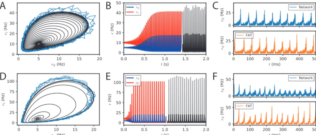
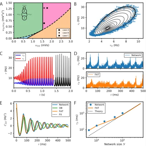
Fig 1. Dynamical regimes of an E-I module. (A) Stability and instability of the module steady discharge as a function of synaptic coupling. Stable regions with complex eigenvalues (green) and real eigenvalues (light blue) and unstable regions with complex eigenvalues (purple) and real eigenvalues (orange) are shown for the stationary state r(s)_E = 5 Hz, r_I(s) = 10 Hz. Inset: sketch of the excitatory and inhibitory neuronal populations (the E-I module) and their synaptic interactions. The parameters for the three cases shown are: A - wEE = 1.6 mVs,

wIEwEI = 0.64 mV2s2 ; B - wEE = 1.6 mVs, wIEwEI = 1.28 mV2s2; C - wEE = 1.76 mVs,

wIEwEI = 1.28 mV2s2. We use the parameters of case A (solid circle) throughout the remainder

of this article; for cases B and C, see Fig. S2. (B,C) Oscillations of the discharge rates rE, rI

of the E-I populations in the rate-model description, (B) as rI vs. rE or (C) as a function of

time (blue, excitatory population; red, inhibitory population) for parameters corresponding to case A in panel (A) with wIE= 2 mVs, wEI = 0.32 mVs (the corresponding effective constants

are α = 2.33, β = 2.15). Oscillations in a spiking network with a large number of neurons (N = 106, resampled with time bin ∆t = 0.1 ms) are also shown in (B) (blue line) and (C) (black and gray lines). (D) Time traces of the excitatory activity in a spiking network with smaller number of neurons (N = 104_{) and the corresponding stochastic rate model Eqs. (5,6)}

(sampled with time bin ∆t = 0.1 ms). (E) Autocorrelation of the excitatory activity for the spiking EIF module (N = 104_{, solid blue) and the adaptive rate model (solid orange). The}

autocorrelation for the rate model with the adaptive timescale of ref. [48] is also shown (solid green). The fit of the analytical expression Eq. (56) for the autocorrelation to the adaptive rate model (shown in dashed black) allows to obtain the module’s autocorrelation decay time τD.

(F) The decorrelation time τD shown for spiking modules (solid blue dots), for FAT modules

parameters corresponding to one such point are indicated in Fig. 1A (solid black circle) and used as reference for the figures of the present paper. The corresponding limit-cycle oscillations are shown in Fig. 1B,C. Two other representative sets of parameter values are also indicated in Fig. 1A (solid losange and square) and the corresponding dynamical traces are shown in Fig. S2.

The rate-model description is compared to simulations of spiking networks (see Methods: Simulations of spiking networks) in Fig 1. The rate-model deterministic activity trace accounts well for the network activity when the number N of spiking neurons is very large (N ∼ 106) and stochastic effects at the level of the population are negligible, as shown in Fig 1B,C.

Our E-I module with unstructured connectivity is, however, intended to represent local interactions at a scale comparable to that of a cortical column [56, 57], which is estimated to comprise a smaller number of neurons (N ∼ 104_{− 10}5_{). In this case, simulations show}

that the network population activity has a significant stochastic component, as seen in Fig. 1D. Auto-correlograms of the E population activity display decreasing oscillatory tails reflecting the corresponding dephasing of oscillations (Fig. 1E).

We take into account these stochastic effects in the rate-model description by remem-bering that, in a sparsely synchronized spiking network [30], the global network activity retains a stochastic component due to the finite numbers NE, NI of excitatory and

inhibitory neurons in the network, even for constant external inputs. We follow ref. [39] and assume that, in the SSO regime, the probability of an excitatory (resp. inhibitory) spike between the times t and t + ∆t is given by ΦE[IE(t)]∆t (resp. ΦI[II(t)]∆t), and

spikes being independently drawn for each neuron in the network. This leads to replacing the deterministic relations rE(t) = ΦE[IE(t)] and rI(t) = ΦI[II(t)] by stochastic versions

coming from Poissonian sampling, an approximation that has previously been shown to be quite accurate when neurons are sparsely synchronized [39],

rE(t) = ΦE[IE(t)] + p ΦE[IE(t)]/NEξE(t) , (5) rI(t) = ΦE[II(t)] + p ΦI[II(t)]/NIξI(t) , (6)

where ξE(t), ξI(t) are independent white noises (hξE(t)ξE(t0)i = hξI(t)ξI(t0)i = δ(t − t0),

hξE(t)ξI(t0)i = 0) and Ito’s prescription is used [58]. Eq. (5,6) transform the deterministic

rate equations into stochastic ones with a noise amplitude that is inversely proportional to the size of the population

Accounting in this way for finite-size fluctuations allows the FAT rate-model descrip-tion to reproduce quite well the sparsely synchronized oscilladescrip-tions in a moderately-sized spiking network (Fig. 1D). The similarity between the spiking network and the stochastic FAT model can be quantitatively assessed by computing the autocorrelations of the E-I module excitatory population activity, CEE(t − t0) = hrE(t)rE(t0)i − hrEi2. As shown

in Fig. 1E, the stochastic FAT model accurately describes the network autocorrelation. It should be noted that the added stochastic terms in the rate equation description have no free parameters, they are entirely determined by the assumption (admittedly approximate) that the instantaneous network spike rate is the product of an underlying Poissonian process.

Stochastic dephasing of oscillations leads to an exponential decrease of the autocorre-lation amplitude with a characteristic time τD,

|CEE(t)| ∼ exp(−t/τD) . (7)

The time τDincreases with the number of neurons in the E-I module as shown in Fig. 1F.

Well-known results are available to analytically describe dephasing due to weak noise [19, 25, 51, 52], namely in the present case when the E-I module comprises large numbers of neurons and finite-size fluctuations around the deterministic limit cycle

are small (see Methods: Diffusion of the oscillation phase of an E-I module with a finite number of neurons). For very large numbers of neurons, the activities of the two populations (rE(t + φ), rI(t + φ)) are oscillatory with rE(t) and rI(t) periodic functions

of time, and the phase φ being arbitrary but constant. Note that in the present work, we define the phase φ to be a variable with the same dimension as time and with a period T equal to the oscillation period. Another usual convention is to consider the phase as a dimensionless variable with a period of 2π. (Therefore rE is here a periodic

function of the phase φ with period T , instead of being a periodic function of a phase with period 2π.) The phases in these two different conventions are simply related by a multiplicative factor of 2π/T .

Stochastic fluctuations in E-I modules with large number of neurons dominantly produce a random drift of the phase φ with a diffusive behavior in time,

h[φ(t) − φ(0)]2_{i = D}

Nt . (8)

Similarly to the amplitude of the finite-size fluctuations of activity, the diffusion constant DN vanishes as the numbers NE of excitatory neurons and NI of inhibitory neurons in

the module grow,

DN = DE NE +DI NI . (9)

The constants DE and DI can be expressed and computed in terms of integrals along

the deterministic limit cycle [19] (Eqs. (53,54) in Methods). This provides an explicit expression of the decorrelation time as a function of DN and the period of the limit

cycle, τD= 1 2π2 T2 DN . (10)

Eq. (10) predicts that the dephasing time increases linearly with the size N of the E-I module. Expression (10) is displayed in Fig. 1F. It agrees well with the simulation results for large N . Quantitative agreement deteriorates as N diminishes and fluctuations become stronger. Fluctuations then strongly affect the shape of limit cycle itself and the description by a pure dephasing becomes less accurate.

Dynamical regimes of two oscillatory E-I modules coupled by

long-range excitation

We start by considering the simplest case of coupling between distant modules, namely two identical E-I modules coupled by long-range excitation. In spite of the addition of the adaptive timescale in the rate model we use, the results we obtain are very similar to results [21, 22] obtained for the classic Wilson-Cowan model [20]. It matters for synchronization whether long-range excitation targets only excitatory neurons or both excitatory and inhibitory neurons. We thus distinguish the two cases.

Long-range excitation targeting excitatory neurons

We analyze the synchronization properties between two E-I modules with oscillatory activity when long-range excitation only targets excitatory neurons, the “E → E” connectivity case depicted in Fig. 2A.

The dynamics of two coupled E-I modules are described in the rate-model framework (3,4) by

τE(IE,1)

dIE,1

dt = −IE,1+ I

ext

E + wEE[(1 − flr)rE,1+ flrrE,2] − wEIrI,1 (11)

τI(II,1)

dII,1

dt = −II,1+ I

ext

B

1

2

3

4

5

6

!

"

#

$

%

&

Figure 2

Fig 2. (see next page)

with the same two equations with permuted indices 1 and 2 describing the dynamics of module 2.

We first consider the dynamics of this two-module network for two coupled deter-ministic FAT rate models, when the firing rates, rE,n and rI,n for n = 1, 2, are given

in terms of the respective currents by the f-I curve (Eq. (2)). Mathematical analysis and simulations show the existence of a number of different dynamical regimes. In order to obtain a precise view of the various cases as a function of the different synaptic couplings, we choose the parameters of the E-I modules so that they remain at a fixed oscillatory location in the parameter diagram of Fig. 1A. This fixes in each module the total strength of recurrent excitatory connections wEE and the total inhibitory feedback

wIEwEI, and leaves as variable parameters the strength of excitation on inhibitory

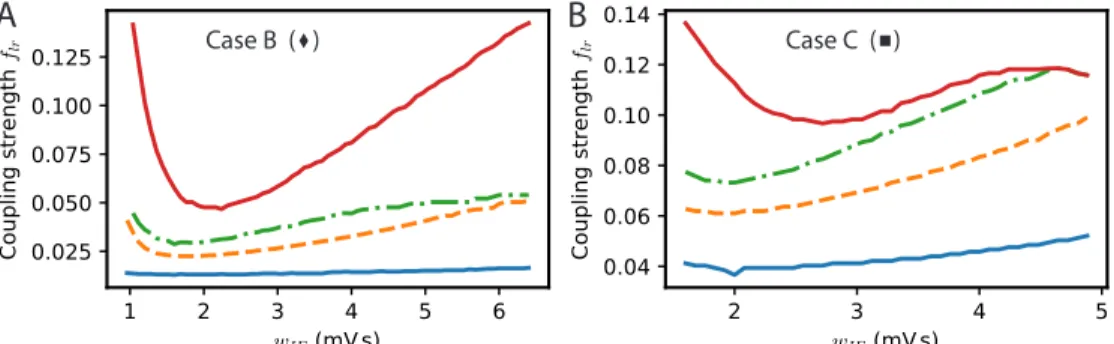
Fig 2 (previous page). Synchronization and dynamical regimes for two E-I modules coupled by long-range excitation. (A) Sketch of the coupled E-I modules and their synaptic interactions. Top: In the E → E connectivity case, long-range excitation only targets excitatory neurons in other modules. Bottom: In the E → E, I connectivity case, long-range excitation targets excitatory and inhibitory neurons in distant modules in equal proportion. (B) Different dynamical behaviors for the coupled modules as a function of the coupling strength flrand

the synaptic excitatory strength on inhibitory neurons wIE. The labeled points (solid black

circles) mark the parameters of the dynamical regimes shown in (B1-6) , the cross (light grey) corresponds to the parameter used in Fig. 3A. (B1) Fully synchronized state for sufficiently strong long-range excitation; flr= 0.03. (B2) Finite phase difference: the activity of one module

is greater than the other, the amplitudes of their oscillatory activities are constant in time but the phases of their oscillations are different; flr= 0.025. (B3) Modulated dominance: one of

the two modules is more active than the other but the amplitudes of the oscillatory activities of both modules vary themselves periodically in time; flr= 0.02. (B4) Alternating dominance:

the activities of the two E-I modules successively dominate; flr= 0.015. (B5) Antiphase regime

at very low coupling and strong local excitation on inhibitory neurons; flr= 0.001. (B6) Finite

phase difference regime at very low coupling and weak local excitation on inhibitory neurons; flr= 0.001 and wIE= 1.44 mVs. (C) The synchronization function governing the evolution of

the relative of two weakly coupled modules in the E → E connectivity case. Modules with weak local excitation of inhibitory neurons wIE (blue solid line), strong local excitation of inhibitory

neurons (orange dashed-dotted line) and wIEclose to the threshold strength of local excitation

separating the two regimes (red dashed line). (D) The synchronization function governing the evolution of the relative phase of two weakly coupled modules in the E → E, I connectivity case. The fully synchronized state is the only stable state (zero-crossing with negative slope) for the three shown wIE values. (E) The difference of excitatory activity between the two

modules decreases exponentially (wIE= 2 mVs, flr= 0.001). (F) The measured exponential

restabilisation in two-modules FAT simulation with E → E, I connectivity (crosses, flr= 0.001)

matches well the prediction of Eq. (15) and Eq. (66) (solid black line).

and the fraction flr of excitatory connections on excitatory neurons that corresponds

to long-range excitation. The found dynamical regimes of the two E-I networks are displayed in Fig. 2B as a function of wIE and flr for one of our reference points (case A

marked by the black solid circle in Fig. 1A; the analogous diagrams for the two other points are shown in Fig. S3). The individual panels Fig. 2B1-6 show representative traces of the activities of the two excitatory populations in the different regimes. We describe them in turn.

When the E-I modules are not coupled, each of them oscillates with a period T and an arbitrary phase with respect to the other module. For very weak long-range excitation, the effect on each E-I module of the excitatory inputs coming from the other one simply leads to a slow change of the phase of its oscillation [19, 21, 23, 24]. The synchronization dynamics itself can be characterized by the evolution of the relative phase ∆φ between the oscillations of the two modules. For ∆φ = 0, the two modules oscillate in phase whereas for ∆φ = T /2 they oscillate in antiphase. The evolution of ∆φ is found to be governed by the following dynamics [19, 21, 23, 24] (see Methods: Synchronization function for two weakly coupled E-I modules):

d∆φ

dt = flrSE(∆φ) . (13)

The function SE(∆φ) is shown in Fig. 2C for different synaptic parameter values wIE.

For two identical modules, symmetry implies that the phase differences ∆φ = 0 and ∆φ = T /2 are always zeros of SE. Therefore, in-phase as well as antiphase oscillations

are always possible oscillating states. In the present case, the positive slope of the zero-crossing at ∆φ = 0, S_E0 (∆φ) > 0 shows that in-phase oscillations are always unstable. When local excitation targets sufficiently strongly interneurons, i.e. for wIE > w∗IE,

S_E0 (T /2) < 0 and antiphase oscillations are the only possible stable phase difference. An example of such oscillations is displayed in Fig. 2B5. On the contrary for wIE< w∗IE,

both in-phase and antiphase are unstable. The function SE(∆φ) displays a new zero at

a non-trivial ∆φ with a negative slope (Fig. 2C) and the two modules stably oscillate with this non-trivial phase difference (Fig. 2B6). Such a synchronization regime was also obtained [21] for the classic Wilson-Cowan rate model [20].

For a larger strength of long-range excitation, the interaction between the two modules does not reduce to changing their oscillation phases. Nonetheless, the stability of the in-phase oscillations can be computed (see Methods: Stability analysis of full synchronization for two coupled E-I modules). The analysis shows that fully synchronous oscillations (Fig. 2B1) are stable when long-range excitation is sufficiently strong. This actually happens for a relatively weak long-range excitation strength, at about flr ∼ 2 − 7%,

depending on the strength wIE of the local excitation on the inhibitory population in

each module (Fig. 2B).

More complex dynamical regimes hold for intermediate strengths of the long-range excitation, below that required for full synchrony and above the excitation strength leading to finite-phase difference phase at very low flr. A first decrease of flr below that

necessary for full synchrony leads to a phase where the two-modules oscillate at the same frequency and different phases. In contrast to the finite-phase difference at very low flr,

oscillation amplitude in one module strongly dominates the other one, as illustrated in Fig. 2B2. This finite phase difference regime itself looses stability with a further decrease of flr and is replaced by a “modulated dominance” regime: beta/low gamma oscillations

in one module continue to be of larger amplitude in one module than in the other one but these two unequal amplitudes are themselves modulated at a very low frequency in the 1 Hz range, as shown in Fig. 2B3. This regime stems from a Hopf bifurcation of the finite-difference regime, with the unusual low frequency coming from the small value of flr (see Methods: Stability analysis of full synchronization for two coupled E-I

modules). A further decrease of flr transforms the modulated-dominance regime into

an “alternating dominance” regime: oscillations in one module dominate the oscillations in the other one, but the dominant module switches periodically, again with a slow frequency in the 1 Hz range, as illustrated in Fig. 2B4. Similarly to modulated dominance, alternating dominance stems from a Hopf bifurcation of the antiphase regime at very low flr, when flr is increased. A sequence of bifurcations and dynamical states similar

to the one reported in Fig. 2 has been described long ago [22] for the Wilson-Cowan rate model upon increase of the excitatory coupling between the two modules. The regimes that we call here “alternating dominance” and “modulated dominance” are referred to as “antisymmetric torus” and “nonsymmetric torus” in ref. [22] and a short discussion of the transition between them is provided.

Long-range excitation targeting excitatory and inhibitory neurons

We now consider the case in which long-range excitation targets both excitatory and inhibitory neurons with strengths proportional to that of local excitation. In this case, Eq. (12) is replaced by τI(II,1) dII,1 dt = −II,1+ I ext I + wIE[(1 − fr)rE,1+ frrE,2] (14)

with the same equation with permuted index 1 and 2 to describe the dynamics of the inhibitory population of module 2.

In this “E → E, I” connectivity case, sketched in Fig. 2A, long-range excitation is found to always have a synchronizing effect.

For very weak coupling, the synchronization dynamics can be reduced as above to the evolution of the relative phase of the two modules. It is described by Eq. (13) with the

Constant Value Definition

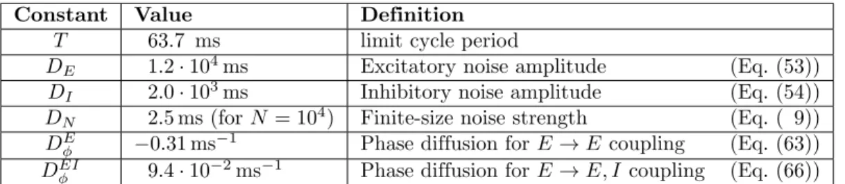
T 63.7 ms limit cycle period

DE 1.2 · 104ms Excitatory noise amplitude (Eq. (53))

DI 2.0 · 103ms Inhibitory noise amplitude (Eq. (54))

DN 2.5 ms (for N = 104) Finite-size noise strength (Eq. ( 9))

DE

φ −0.31 ms−1 Phase diffusion for E → E coupling (Eq. (63))

DEI

φ 9.4 · 10−2ms−1 Phase diffusion for E → E, I coupling (Eq. (66))

Table 1. Computed constants. Values of the constants defined in the text for the E-I module limit cycle with the reference parameters (solid circle in Fig. 1A) wEE = 1.6 mVs,

wEI = 0.32 mVs, wIE= 2.0 mVs.

function SEI(∆φ) plotted in Fig. 2D. For a small phase difference, SEI(∆φ) behaves as

SEI(∆φ) ' −2∆φ DEIφ , (15)

with the constant DEI

φ depending on the characteristics of the oscillation cycle (see

Eq. (66) in Methods). The constant DEI

φ is found to be positive (see Table 1 for its value

at the reference point wIE = 2 mVs). Eq. (15) shows that a zero phase lag between the

two modules is a dynamically stable configuration, in contrast to our previous results for E → E connectivity (compare with Fig. 2C). Eq. (15) predicts that an initial activity difference between two oscillating E-I modules should vanish exponentially. As shown in Fig. 2E, this is indeed observed in simulations with a rate of decrease that agrees well with the one predicted by Eq. (15) (see Fig. 2F).

We have checked that this synchronizing effect of long-range excitation persists for stronger long-range excitation strengths. We have found the two-module fully synchronized regime to be linearly stable for all couplings for which we computed its stability matrix (see Methods: Stability analysis of full synchronization for two coupled E-I modules). Moreover, numerical simulations with different initial conditions did not show any other stable pattern. Therefore, we conclude that in the context of the present model with instantaneous synapses and no propagation delays, long-range excitation with E → E, I connectivity between two E-I modules always tends to fully synchronize their activities.

Comparison with spiking networks and influence of stochastic activity fluctuations For a single E-I module, we already found a good match between the oscillatory dynamics in the rate-model framework and simulations of a spiking E-I network, as described in the first section of the results. Finite-size fluctuations were found to play an important role for modules of moderate sizes and were found to be well accounted for by our stochastic rate model. We now pursue this comparison in the two-module case by taking the firing rates rE,nand rI,nin Eqs. (11),(12) or (14) expressed in terms of the respective currents

by the stochastic relations Eq. (5) and Eq. (6) which account for the finite number of neurons in the networks.

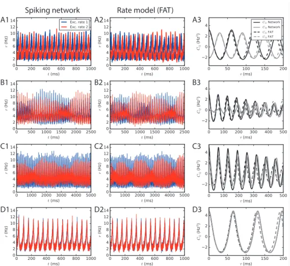
Fig. 3 shows the close correspondence between the rate-model results and networks with a large number of neurons (N ∼ 106_{) for E → E connectivity. The different}

dynamical regimes for two E-I modules coupled by long-range E → E connectivity are all observed in simulations of networks spiking neurons. Both antiphase (Fig. 3A), alternating dominance (Fig. 3B), modulated dominance (Fig. 3C) and full synchrony (Fig. 3D) are observed for parameters that quantitatively correspond to those predicted by the rate-model analysis. Similarly, in the case of E → E, I connectivity, two large E-I modules oscillate in full synchrony as predicted by the rate description (not shown).

Spiking network Rate model (FAT) A1 A2 A3 B1 B2 B3 C1 C2 C3 D1 D2 D3

Figure 3

Fig 3. Two large E-I modules coupled by long-range excitation. (1,2) E-I modules with a large number of neurons, N = 1.6 · 106, and E → E connectivity. The different dynamical regimes depicted in Fig. 2 for different coupling strengths are clearly visible both in (1) spiking network simulations and in (2) the corresponding rate-model simulations. The respective auto-and crosscorrelations of the excitatory activities are shown in panels (3). The coupling strengths are as follows: (A) flr= 0.01 (light grey cross in Fig. 2B), (B) flr= 0.015, (C) flr= 0.02, (D)

flr= 0.05.

For smaller number of neurons, stochastic effects compete with deterministic effects both in simulations of spiking networks and in the rate-model description, when stochas-ticity arising from finite-size effects is accounted for. Interestingly, both descriptions continue to agree well when fluctuations play a major role in the dephasing of the two E-I modules, as shown in Fig. 4.

For E → E connectivity, the correlation between the activities of the two networks clearly displays the signature of the antiphase regime at weak coupling for N = 2 · 105

neurons, whereas it is not apparent for N = 104_{when stochasticity is stronger (Fig. 4A,B).}

At larger coupling, even small fluctuations lead to modules exchanging their roles and make more complex regimes difficult to identify even for N = 2 · 105 _{neurons. This is}

illustrated by simulations with a coupling parameter in the modulated dominance regime (flr = 0.02, Fig. 4C). The ratio of cross- and auto-correlation functions at zero time lag

shows that the transition between different regimes as a function of coupling is blurred by stochasticity as N decreases (Fig. 4E,F).

!

"

#

$

%

&

'

(

)

*

+

,

Excitatory-to-excitatory cross-coupling only

Excitatory-to-excitatory & excitatory-to-inhibitory cross-coupling

Figure 4

Fig 4. Stochastic effects due to network size for two E-I modules coupled by long-range excitation. Auto- and crosscorrelations C11 and C12of the activities of E-I modules

with a finite number of neurons N = 104and 2 · 105 for different coupling strengths flr= 0.01

and 0.02 with long-range excitation targeting only excitatory populations (A-D) or targeting both excitatory and inhibitory neurons (G-J) (parameter values are stated in the panels’ lower left corner). Summary plots with the ratio of equal-time crosscorrelations over autocorrelations for varying N and flrare shown in (E,F) and (K,L), respectively. In the E → E case, oscillatory

synchrony between the two modules disappears when the coupling strength flrdiminishes ((C)

vs. (D)), but the dynamical regimes of Fig. 2 are blurred by stochastic effects when the network size N decreases ((A,B) vs. (C,D)). In the E → E, I case, no other dynamical regimes than oscillatory synchrony are expected, but synchrony increases both with coupling strength flr

and, more strongly, with network size N .

this case, two effects can be observed. On the one hand, synchrony decreases at fixed coupling strength when N is decreased due to larger noise (Fig. 4G,H). On the other hand, synchronization of the two networks increases when coupling strength increases at fixed N (fixed noise) as shown in Fig. 4G,I and Fig. 4H,J. Both effects are quantified in Fig. 4K,L.

One should note that whereas the precise targeting of the long-range excitation plays a crucial role in the instability of in-phase oscillations for large networks (N ∼ 106_),

it is much less important for smaller (N ∼ 104_{) networks. For these smaller networks,}

the dominant role of fluctuations in the dynamics of the two individual E-I modules modifies the connectivity synchronization properties. It leads to similar synchronization

effects of long-range excitation, whether one module only targets the other E population (E → E connectivity) or targets both E and I populations in the other module (E → E, I

connectivity) (compare Fig. 4B to Fig. 4H).

Analysis of the competition between synchronization and noise

We thought it interesting to try and analyze more precisely the competition between synchronization and stochastic fluctuations, given that it arises for E-I modules of biologically realistic sizes. We chose to precisely study the case of E → E, I connectivity when stochastic fluctuations simply compete with full synchronization promoted by long-range connectivity. We developed two approaches which both assume that fluctuations are of an amplitude moderate enough that they can be treated as perturbations of the deterministic limit cycle.

A classical approach is available for weakly coupled modules and small noise. It was previously used to study noisy coupled oscillators [19] as well as neural systems [25]. In the present case, the outcome of this approach is that finite-size fluctuations in the rate-model description add a stochastic component to the previous Eq. (13) for the phase difference between the two modules (see Eqs. (78) and (84) in Methods). (It also provides an estimate to the small shift of oscillation frequency due to small noise [51, 52] which we do not consider here). This leads to a very explicit quantification of the difference of oscillation phases between the two modules induced by fluctuations,

h(φ1− φ2)2i =

DN

2flrDφEI

. (16)

In this expression, the constant DN is simply the amplitude of stochastic fluctuations

in a single module (Eq. (9)), whereas flrDEI quantifies the synchronization strength

due to long-range connectivity (Eqs. (66) and (15)). As intuitively expected, the mean square phase difference between the two oscillators increases with the noise strength and decreases when the synchronization strength increases.

Eq. (16) provides a simple estimate of the competition between stochastic dephasing and synchronization. In order to compare it to numerical simulations, one can compute the respective phase of oscillations of two oscillatory E-I modules. Alternatively, Eq. (16) can be transformed into a prediction of the average spike-rate difference between the two modules, taking into account that the firing rate is a periodic function of the oscillatory phase (Eq. (82) in Methods). The latter is chosen to compare with results of numerical simulations of both FAT rate-model and spiking network implementations of two coupled E-I modules in Fig. 5. The mean square difference of excitatory rates between the two modules are quite comparable in the noisy FAT (Fig. 5A) and spiking networks (Fig. 5B), again showing the quantitative accuracy of the FAT rate-model description.

However, Fig. 5 shows that the predicted rate difference fluctuations obtained from Eq. (16) (“phase approximation” in Fig. 5) are accurate only for very small coupling between the two modules.

The underlying assumption in Eq. (16) is that the phase difference plays a dominant role in the difference of activities between the two E-I modules because the phase difference mode has a much smaller restoring strength than the other (amplitude) mode between the two modules. The respective eigenvalues of the two modes are shown in Fig. 6G as a function of the fraction of long-range connection flr. Indeed, for weak

coupling (flr 1), one eigenvalue µA1 is close to 1, so that the restoring strength 1 − µA1

of the corresponding (phase) mode is much smaller than 1 − µA

2, the restoring strength

of the other mode. However, an explicit computation shows that µA

1 quickly decreases as

flr increases (see Eq. (76) in Methods). Therefore, the two modes soon play comparable

Figure 5

Fig 5. Competition between synchronization and noise for two E-I modules with E → E, I connectivity: theory vs. simulations. The variance of excitatory activity between the two modules hδr2

Ei = h(r1,E− r2,E)2i/2 is shown as a function of coupling strength flr.

(A) Simulations of the stochastic rate model (FAT, duration 100 s, averaged over 3 repetitions) for different noise strengths (color symbols), as specified in the insert in term of the number of neurons N in the individual E-I module. These simulation results are plotted against theoretical predictions with different approximations. For very small coupling strengths, the phase approximation with the full limit cycle dynamics (Eqs. (16, 82), dotted lines) gives a good account of the observed synchronization, while for larger couplings both phase and amplitude modulations have to be considered (two-mode calculation, Eq. (97), solid black line). Note that for very small couplings, the two-mode calculation coincides with the phase approximation with linearized limit cycle dynamics (Eqs. (16,80), dashed black line), which does not take into account the periodicity of the firing rate as a function of the phase and which predicts an unphysical diverging activity difference for vanishing coupling. (B) Same as in (A) with the results for the network simulations of Fig. 4K,L (colored solid lines corresponding to different E-I module sizes, as sprecified in the inset), shown as hδr2

Ei = C11(0) − C12(0).

We developed another approach, valid for small noise but for arbitrary coupling flr, in

order to check this origin of the inaccuracy of Eq. (16) as well as to obtain a quantitatively precise description of the competition between synchronization and stochasticity. The approach is simply based on accounting for the effect of stochastic perturbations at a linear level around the fully synchronized state where all modules are in the exact same states (see Methods: Competition between synchronization and stochasticity for two coupled E-I modules of finite size. Weak noise at arbitrary coupling). As shown in Fig. 5, this two-mode computation produces precise estimates of the mean square excitatory rate difference of the two modules, h(r1,E− r2,E)2i, even for modules with

only 104 _{neurons when stochasticity is quite high. This second approach is thus quite}

successful in quantitatively capturing the observed competition between synchronization and stochasticity.

Phase gradients in a chain of oscillatory E-I modules coupled by

long-range excitation

Having analyzed the synchronization dynamics and effects of finite-size fluctuations for two E-I modules, we now turn to a fuller description of spatially-structured connectivity. We consider a chain of E-I modules, with each module’s long-range excitation targeting other modules in a distance-dependent way. Interestingly, the effects that we uncovered in the two-module setting, such as desynchronization at weak coupling for E → E connectivity and competition of synchronization with stochastic finite-size fluctuations, reappear in a more elaborate form. Moreover, the computational techniques that we developed for the two-module case turn out to be directly applicable to the chain of modules.

!

"

#

$

%

&

'

(

)

***

***

Figure 6

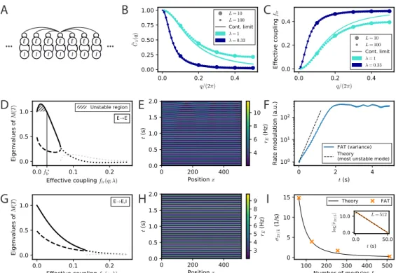
Fig 6. Spontaneous appearance of phase gradients in a chain of E-I modules. (A) Sketch of the chain of E-I modules coupled by long-range excitation. Excitatory neurons in one module target excitatory neurons (E → E) or excitatory and inhibitory neurons (E → E, I) in the other modules with a distance-dependent excitation profile. (B) Fourier transform of the coupling function ˜Cλ(q) (Eq. (106)) for perturbations of wavenumber q when the long-range

excitation has an exponential profile (Eq. (20)), for space decay constants λ = 1 (turquoise) and λ = 0.33 (dark blue). For λ  1, the chain of modules can be approximated by a continuous system. (C) Effective long-range coupling flr(q; λ) = (1 − ˜Cλ(q))/2 for perturbations

of wavenumber q. (D) Stability spectrum for perturbations of wavelength q as function of the effective coupling flr(q; λ) for E → E connectivity. For small coupling strengths, i.e. long

wavelengths, the largest eigenvalue (thick solid line) is larger than 1, and the perturbations are unstable (flr< flr∗, hatched region). While both eigenvalues are real and positive for small

coupling strengths, they become complex conjugated for larger couplings (real part, thick dotted black line; imaginary part, thick dotted grey line). (E) Excitatory activity rE for a chain of

deterministic E-I modules over time (L = 512, with 0.1 mV noise on initial condition). (F) Growth of the variance of excitatory activityPL

n=1(rn,E−PLm=1rm,E/L)2over time, with the

predicted rate for the fastest-growing mode shown on top (dashed black line). (G,H) Same as (D,E) but for E → E, I connectivity. Note that all modes are stable (G) and no instability develops over time (H). (I) Rate of decay of longest wavelength perturbation σ2π/Lfor different

chain lengths L (orange crosses) against the theoretical prediction (Eq. (23), black line). Inset: Decay of the spatial modulation of excitatory activity over time (L = 512). For all simulations shown, λ = 1/3.

Spontaneous appearance of phase gradients due to long-range excitation specifically targeting excitatory neurons

The setting of our analysis is sketched in Fig. 6A. E-I modules with locally unstructured connectivity are coupled by long-range excitation. For E → E connectivity, the

dynamics of L coupled E-I modules are described in the rate-model framework (3,4) by τE(IE,n) dIE,n dt = −IE,n+ I ext E + wEE X m=1,··· ,L C(n, m)rE,m− wEIrI,n (17) τI(II,n) dII,n dt = −II,n+ I ext I + wIErE,n (18) with C(n, m) = C(|n − m|).

For E → E, I connectivity, Eq. (18) is replaced by τI(II,n) dII,n dt = −II,n+ I ext I + wIE X m=1,··· ,L C(n, m)rE,m. (19)

The connection strength decreases monotonically with the distance l between modules [17], as described by the function C(l). Our analytical expressions are valid for a general functional form. For the numerical simulations, we have chosen, for illustration, an exponential decrease which appears compatible with experimental data in the primate motor cortex [16]. We specifically take

C(l) = Aλ[exp(−λ|l|) + exp(−λ(L − |l|))] , Aλ=

1 − exp(−λ)

[1 − exp(−λL)][1 + exp(−λ)] (20) where Aλ implements the normalizationPl=0,··· ,L−1C(l) = 1. The second exponential

corresponds to choosing periodic boundary conditions for the chain. While this is not realistic for the cortex, it minimizes boundary effects in the simulations and should not significantly modify the results in the regime when L is large compared to 1/λ (i.e., when exp(−λL)  1).

We first analyze the dynamics in the framework of deterministic rate equations, before considering the effects of fluctuations and comparing with spiking networks in the next section.

A perfectly synchronized oscillating chain, with zero phase difference between the oscillations of different modules, is always a possible network state at the level of the rate-model description. It needs however to be tested whether full synchronization is resistant to perturbations or whether some perturbations are amplified by the dynamics and full synchronization is unstable. Interestingly, the linear stability analysis of a periodic lattice such as the considered 1D chain, exactly reduces to that of a two E-I module network with an effective coupling flr. More precisely, any small perturbation

of the fully synchronized state is the linear sum of periodic perturbations with different wavenumbers q which evolve independently of each other. Perturbations of wavenumber q evolve in the same way as perturbations in the two E-I module network considered in the previous section, provided the coupling in the two-module network is chosen as

flr(q) = [1 − ˜Cλ(q)]/2 , (21)

where ˜Cλ(q) is the Fourier transform of the long-range excitation profile C(l) (Eq. (106)

in Methods). C˜λ(q) and the corresponding “effective” coupling in the two-module

network, flr(q), are displayed in Fig. 6B,C for an exponentially decreasing long-range

excitation profile C(l) ∼ exp(−λ|l|). It is seen in Fig. 6C that small wavenumbers q correspond to weak effective coupling flr(q), with flr(q) → 0 when q → 0. While deriving

the exact relation (21) requires mathematical analysis (see Methods: Stability analysis of full synchronization for a chain of oscillatory E-I modules), it can be intuitively understood. For perturbations of small wavenumbers (q → 0), only distant parts of the chain are in distinct oscillating states. The relative dynamics of these distant parts is

thus effectively only weakly coupled by excitation since long-range excitation decreases with distance. The relation (21) allows one to directly transcribe for the E-I module chain the results previously obtained for the two E-I module case. As before, we compare two connectivities for long-range excitation.

We first consider the case of E → E connectivity, when long-range excitation only targets excitatory neurons. The effective coupling flr(q) decreases monotonically with

the wavenumber q and vanishes as q → 0. The stability diagram displayed in Fig. 2B then shows that full in-phase synchronization is unstable for chains sufficiently long to accommodate modulations of small enough wavenumber q. The associated stability eigenvalues are shown in Fig. 6D. In-phase synchronization is unstable when flr becomes

smaller than a critical f∗

lr that depends on the single E-I module synaptic parameters.

For the the chain of modules, this implies that spatially-periodic perturbations grow when their wavenumber q lies below a critical q∗, defined by

cos(q∗) = 1 − 2f ∗ lrcosh(λ) 1 − 2f∗ lr , or q∗' s 2f_lr∗ 1 − 2f∗ lr λ , (22)

where λ controls the exponential decrease with distance of the long-range excitation. The second equality in Eq. (22) is valid for small λ; the used approximate relation between flr and q is shown in Fig. 6C, it can be seen that it is already very accurate for λ = 1/3.

Eq. (22) predicts that for a network of sufficient spatial extent L > 2π/q∗, spontaneous phase gradients should appear along the chain. This is confirmed by direct numerical simulations of the rate-model equations, shown in Fig. 6E. The exponential growth of the modulation of excitatory activity along the chain is shown in Fig. 6F, starting from a weakly perturbed fully synchronized state. This directly confirms the linear instability of full synchronization. One further notable feature in Fig. 6E is that the phase gradients develop on a spatial scale that is quite long (i.e. ∼ 30 modules) compared to the spatial scale of the long-range excitation profile C(l) (∼ 1 in Fig. 6D). This stems from the fact that in-phase synchronization is unstable only for small flr(q), that is, for small q or long

wavelengths compared to the characteristic module coupling length. For our reference parameters and wIE = 2 mVs, Eq. (22) gives for the critical wavelength q∗ ' 0.24λ.

Similarly, one obtains qm' 0.15λ for the wavenumber qmof the fastest-growing mode,

which corresponds to the largest eigenvalue in Fig. 6D.

For E → E, I connectivity, when long-range excitation targets both excitatory and inhibitory neurons, the previous two E-I module synchronization analysis shows that full synchronization is stable up to vanishingly low coupling flr. The stability eigenvalues

are shown in Fig. 6G. For all wavelengths, their real part is less than 1. This linear analysis thus predicts that any modulation of activity along the chain should disappear exponentially. This is indeed what is observed in direct simulations of a chain of modules, as illustrated in Fig. 6H. Moreover, our stability analysis shows that the longest wavelength modes are the slowest to vanish. Their relaxation rate is obtained (Eq. (107) in Methods) as σq = DEI φ 2[cosh(λ) − 1]q 2_{. (23)}

The relaxation rate σq vanishes when q → 0 and decreases with increasing modulation

wavelength. The smallest wavenumber that can be accommodated in a chain of L modules is 2π/L. Fig. 6I shows that σ2π/Las given by Eq. (23) precisely describes the

approach to full synchronization in our simulations of a E-I module chains of different lengths with long-range E → E, I connectivity.

Figure 7

!

"

#

$

%

&

'

(

)

*

+

,

Fig 7. (see next page)

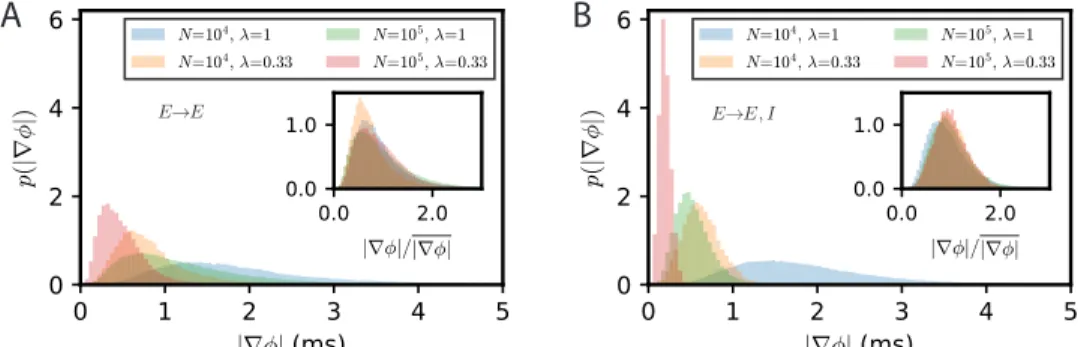
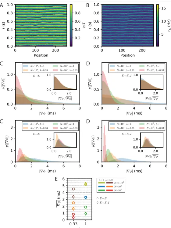
Phase gradients emerging from stochastic fluctuations in E-I modules of finite size Spontaneous stochastic fluctuations of activity are present in each E-I module with a finite number of neurons, as already emphasized. In the two E-I module case, these were seen to compete with synchronization and promote phase differences between different E-I modules. Finite-size fluctuations similarly act in a chain of E-I modules. This is shown in Fig. 7, where the results of stochastic rate-model simulations are displayed for both E → E and E → E, I connectivity. Both the phases of oscillation of different modules (Fig. 7A,D) and the activity of excitatory neurons (7B,E) show that in both connectivity cases differences between neighboring modules are present. The histograms of phase differences between nearest modules are displayed in Fig. 7C,F for E → E and for E → E, I connectivity, respectively. In both cases, differences in phases decrease when the number of neurons in the modules increases, i.e., when stochastic fluctuations decrease. They also decrease when the range of long-range excitation increases and neighboring modules become more strongly coupled. The similarity between the two connectivity cases shows that stochastic fluctuations play the dominant role in creating phase differences between neighboring modules, for modules of size lower than N = 105.

The stochastic fluctuations along the two chains of E-I modules are further quantified in Fig. 7G,H by computing the power in different spatial modes. These clearly show that for both connectivities, power is highest in the longest wavelengths. This qualitatively

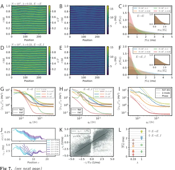
Fig 7 (previous page). Appearance of phase gradients and stochastic fluctuations in a chain of E-I modules. (A,B) Simulation of the stochastic rate model (FAT) for a chain with E → E connectivity, a space constant λ = 0.33 and network size N = 104. (A) Instantaneous phase as obtained from the Hilbert transform of bandpass-filtered excitatory activity, where the (unfiltered) rates are shown in (B). (C) Distributions of local phase gradients ∇φ = φx+1− φx for different noise strengths and space constants for E → E connectivity.

Inset: distributions of gradients normalized to the respective mean value. (D,E) Phase and excitatory activity for the same parameters as in (A,B) but with E → E, I connectivity. (F) Same as in (C) but for E → E, I connectivity. (G,H) Power spectra of the spatial activity profiles (averaged over 5 s) for different module sizes and space constants λ, for E → E (G) and E → E, I (H) activity, respectively. The spectra obtained from spiking network simulations (N = 5000: L = 128; N = 104: L = 32) are shown in light thick lines, spectra obtained from rate-model simulations are shown in dark thin lines (L = 256). (I) Comparison of the spectra obtained from simulations (FAT, solid lines) and theoretical predictions for E → E, I connectivity. Similar to the two-module case, the modes with larger effective couplings are well described by the two-mode calculation (dashed lines, Eq. (136)), while for smaller couplings, or vanishing q, non-linear effects due to the periodicity of the limit cycle, which are not captured by the linearized two-mode dynamics, become dominant. This limit is better captured by the phase approximation and taking the periodicity of the limit cycle dynamics into account (dash-dotted lines, Eq. (123)). Network size N and space constant λ as in (G,H). (J) Example of a spatially extended phase gradient (upper panel) that gives rise to a the apparent propagation from left to right of a (negative) bump of activity in space (lower panel). Phase and excitatory firing rate are shown over a length of 15 modules for different instances in time, see color code legend. (K) Correlation of spatially extended phase gradients ∇φ (averaged over 5 modules and retained when the absolute average gradient is larger than the standard deviation of local phase differences) with phase propagation velocities vφdetermined from frame-to-frame correlations

between spatial phase profiles (see Methods). (L) Summary plot of average phase gradients for different network sizes N and connection decay space constants λ for E → E connectivity (circles) and E → E, I connectivity (diamonds).

agrees with a generalization of the two-module result Eq. (16) for the chain. This result, given in Eq. (127), is obtained by assuming that oscillatory phase differences dominate the fluctuations between modules. While this is true for very long wavelengths, it does not quantitatively agree with the measured spectra for the smaller wavelengths of interest in the present context (Fig. 7I). A generalization of the two-module computation that we developed to take into account both phase and amplitude modes (see Methods: Charac-terization of the E-I module chain stochastic activity profile) is required to quantitatively describe the simulation results, which is also shown in Fig. 7I.

The above results were obtained by simulating chains of E-I modules using the FAT rate-model description. Equivalent simulations for spiking networks are too demanding in computational power for us to perform. We have however checked that for shorter chains of modules (L = 128 for N = 5000, L = 32 for N = 104_{), the stochastic FAT}

rate model reproduces well the results of spiking network simulations (Fig. 7G,H). This renders us confident that this would be the case for longer chains as well.

Phase waves and propagation of activity

We have shown that stochastic fluctuations in a chain of E-I modules create phase differences in the oscillations of E-I modules along the chain. In the presence of phase differences, activity in different modules peaks at different times and may produce “phase waves” (also described as traveling waves, e.g. in [2, p1219]), as shown in Fig. 7J. The propagation velocity vφ of phase waves is kinematically related to the phase gradient

and the distance between E-I modules (which is also the linear size of an E-I module), vφ=

d

∇φ, (24)

where ∇φ denotes the phase variation between neighboring modules (recall that the phase has the unit of time with our convention) and d is the physical distance between these module centers.

These transient phase waves bear some resemblance to the observation of traveling waves in the motor cortex during episodes of beta oscillations [10–14]. Thus, it appears of interest to better characterize them in the present setting and to compare them to propagation of activity. Phase waves covering a notable spatial range correspond to phase gradients that extend over several modules. Although phase differences between modules are mostly correlated on short length scales, extended phase gradients nevertheless exist. For our purpose, we determined gradients of activity that extend over five modules (see Methods: Simulations and numerical analysis. Detection of propagation events in an E-I module chain), and computed the corresponding phase wave velocity. Furthermore, we independently assessed the spatio-temporal propagation of activity for these occurrences by correlating successive frames of simulations (see Methods: Simulations and numerical analysis. Detection of propagation events in an E-I module chain). These two independently measured velocities are strongly correlated as shown in Fig. 7K. In our simulations, phase gradients and the associated phase waves thus explain the detected propagation of neural activities.

The probability distributions of spatially extended phase gradients are shown in Fig. S4, for the two different considered connectivities and two space decay constants λ of long-range excitation, as well as for different numbers of neurons in the E-I modules. The corresponding mean values of these gradients are summarized in Fig. 7L. In order to compare these values to neural recordings, values for the size of an E-I module and the range of long-range horizontal connections should be determined. Data are available for different species and for different areas [16, 17, 59–61]. For instance, for mouse somatosensory barrel cortex, identifying an E-I module with a barrel column would give d ' 175 µm for the distance between neighboring modules (which is also the linear size of an E-I module) and λ ' 0.7 for layer 2/3 horizontal connections since synaptic excitatory charge is measured to decay to 26% two columns away from an excited column [60].

For the motor cortex of adult monkeys, data are available from intra-cortical micro stimulation and recordings with single and multielectrodes [16]. Response amplitudes vary with the protocol and exact location of the electrodes, but a space decay constant of 1.5 mm seems representative. An E-I module size of d ' 500 µm and N ' 2 · 104

neurons then gives λ ' 0.33 for the long-range connectivity. For this last case, our numerical results give ∇φ ' 0.5 ms (E → E, I) or 1 ms (E → E) depending on the precise connectivity (Fig. 7K). With the above estimate of d, Eq. (24) then gives a phase velocity vφ ∼ 1 m/s or 0.5 m/s, respectively. In both cases, this is significantly larger

than the beta wave velocities recorded in the motor cortex of monkeys. Increasing the local noise on each module increases the dephasing between modules, e.g. ∇φ ' 1.4 ms for N = 5 · 103 _{and (E → E, I) connectivity (Fig. 7K), and correspondingly lowers}

vφ. Thus, in this framework, stochastic dephasing between modules could account for

the experimental results only if other sources of “noise” are present beyond the one coming from the finite size of local modules. This would suggest that different E-I modules receive different inputs, shared at the level of individual modules but varying independently from module to module, as further discussed below.

We assessed one other possibility of increasing local noise with respect to the long-range synchronization of neighboring modules. It would consist of diminishing the importance of long-range coupling relative to purely local excitation, without modifying