-1
The Design and Implementation of a 3D Graphics Pipeline
for the Raw Reconfigurable Architecture
by
Kenneth William Taylor
B.S., Computer and Systems Engineering and Computer Science
Rensselaer Polytechnic Institute, 2002
Submitted to the Department of Electrical Engineering and Computer Science
in partial fulfillment of the requirements for the degree of
Master of Science in Electrical Engineering and Computer Science
at the
MASSACHUSETTS INSTITUTE OF TECHNOLOGY
June 2004
@
Kenneth William Taylor, MMIV. All rights reserved.
The author hereby grants to MIT permission to reproduce and distribute publicly
paper and electronic copies of this thesis document in whole or in part.
Author ...
Department of Electrical Engineering and Computer Science
May 20, 2004
Certified by...
/
Accepted by ...
Anant Agarwal
Associate Professor, CSAIL
Thesis Supervisor
Arthur C. Smith
Chairman, Department Committee on Graduate Students
MAssACHUSETTS INS TE OF TECHNOLOGY
The Design and Implementation of a 3D Graphics Pipeline for the Raw
Reconfigurable Architecture
by
Kenneth William Taylor
Submitted to the Department of Electrical Engineering and Computer Science on May 20, 2004, in partial fulfillment of the
requirements for the degree of
Master of Science in Electrical Engineering and Computer Science
Abstract
This thesis presents the design and implementation of a 3D graphics pipeline, built on top of the "Raw" processor developed at MIT. The Raw processor consists of a tiled array of
CPUs, caches, and routing processors connected by several high-speed networks, and can
be treated as a coarse-grained reconfigurable architecture. The graphics pipeline has four stages, and four-way parallelism in each stage, and is mapped on to a 16-tile Raw array. It supports basic rendering functions such as hardware transform and lighting, perspective correct texture mapping, and depth buffering, and is intended to be used as a slave processor receiving rendering commands from a host system. The design process is described in detail, along with difficulties encountered along the way, and a comprehensive performance evaluation is carried out. The paper concludes with many suggestions for architectural and performance improvements to be made over the initial design.
Thesis Supervisor: Anant Agarwal Title: Associate Professor, CSAIL
Acknowledgments
I would like to thank my thesis advisor, Anant Agarwal, for first introducing me to the Raw architecture and all the interesting thesis ideas revolving around that rich project. I also thank Anant for being so patient with me in the hours nearing the submission deadline. I would also like to thank the members of the Computer Architecture Group, who either directly or indirectly assisted me greatly on this project: from the innumerable maintainers of the starsearch testing suite and all its amazingly useful examples, to the maintainers of the BTL simulator (notably, Michael Taylor, who personally fixed one bug just for me), to others such as Paul Johnson who set me up with the CAG computer system, on which I did a large amount of the work for this project.
I also tip my hat to Kurt Akeley and Pat Hanrahan, whose online lectures for their Stanford Real-Time Graphics course originally inspired me to do a graphics architecture project, even though I knew very little about the subject to begin with.
Finally, I would like to send many, many thanks to April for her support and sympathy through the last few weeks of this project, and also for spending a large amount of her time helping me proofread.
Contents
1 Introduction and Motivation 15
1.1 G oals . . . . . 16
1.2 M ethodology . ... .. ... . 16
1.3 Outline of this Thesis ... 16
2 3D Rendering Algorithms 19 2.1 Introduction to 3D Rendering in General . . . . 19
2.1.1 Defining a Scene . . . . 20
2.1.2 Geometry Transformation . . . . 20
2.1.3 Rasterization and Interpolation . . . . 23
2.1.4 Rendering to the Framebuffer . . . . 26
2.2 3D Rendering Implementation of this Project . . . . 27
2.2.1 Geometry Transformation . . . . 27
2.2.2 Rasterization and Interpolation . . . . 29
2.2.3 Texture Mapping and Blending . . . . 32
2.2.4 Rendering to the Framebuffer . . . . 33
2.3 Sum m ary . . . . 33
3 Designing the Parallel Rendering Architecture 35 3.1 Design G oals . . . . 35
3.2 Basic Parallelization . . . . 36
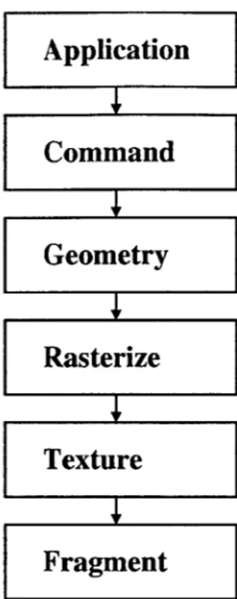
3.2.1 Graphics Pipelines . . . . 36
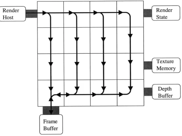
3.2.2 Mapping Parallel Pipelines to the Raw Architecture . . . . 39
3.3 Difficult Design Problems . . . . 39
3.3.1 Distributing Primitives Across the Pipelines . . . . 41
3.3.1.1 Communication in the Raw Architecture . . . . 41
3.3.1.2 Choosing a Network for Commands . . . . 42
3.3.1.3 Techniques for Using the Static Network Dynamically . . . 42
3.3.1.4 Developing the Distribution Algorithm on the Switch . . . 43
3.3.1.5 Improving on Round Robin Distribution . . . . 45
3.3.2 Maintaining Sequential Correctness . . . . 46
3.3.2.1 Dealing With Sequence Number Rollover . . . . 48
3.3.3 Synchronization in the Compositing Stage . . . . 50
3.3.3.1 Attempts at Cache Coherence . . . . 50
3.3.3.2 A Simpler Approach . . . . 51
3.3.4 Other Difficult Issues . . . . 52
3.3.4.2 Switching Modes and Flushing the Pipeline . . . . 52
3.4 Sum m ary . . . . 53
4 Implementation of the 3D Processor 55 4.1 Overview of Architectural Organization . . . . 55
4.2 Detailed Description of Implementation . . . . 58
4.2.1 The Boot Sequence . . . . 58
4.2.2 Command Mode . . . . 58
4.2.2.1 Render State Commands . . . . 62
4.2.2.2 Texture Management Commands . . . . 62
4.2.2.3 Depth and Framebuffer Commands . . . . 63
4.2.2.4 Miscellaneous Commands . . . . 63
4.2.3 Scene Streaming Mode . . . . 63
4.2.3.1 Distributing Commands Among the Pipelines . . . . 64
4.2.3.2 Stage 1 . . . . 65
4.2.3.3 Stage 2 . . . . 68
4.2.3.4 Stage 3 . . . . 69
4.2.3.5 Stage 4 . . . . 69
4.3 Interfacing the Graphics Architecture in a System . . . . 70
4.3.1 The Framebuffer Side . . . . 70
4.3.2 The Host Side . . . . 72
4.4 Summary . . . . 72
5 Testing, Validation and Performance Results 73 5.1 The Testing Framework . . . . 73
5.1.1 The BTL Simulation Environment . . . . 73
5.1.2 Framebuffer Controller . . . . 74
5.1.3 Render Host Interface . . . . 76
5.1.3.1 External Program Control . . . . 76
5.1.3.2 Performance Profiling . . . . 77
5.2 Feature Validation . . . . 78
5.3 Performance Results . . . . 79
5.3.1 Performance Model . . . . 80
5.3.2 Empirical Performance Results . . . . 82
5.4 Sum m ary . . . . 87
6 Improvements and Suggestions for Future Work 89 6.1 Improving Parallelization Efficiency . . . . 89
6.1.1 Reducing Pipelining Overhead . . . . 89
6.1.2 Reducing Parallelization Overhead . . . . 90
6.1.3 Improving Load Balancing . . . . 91
6.1.4 Improving Parallelization Bottlenecks . . . . 92
6.2 Improving Raw Performance . . . . 93
6.3 Scaling the Graphics Architecture . . . . 94
6.4 Ways to Extend This Thesis. . . . . 94
6.5 Sum m ary . . . . 95
A Additional Rendered Images 99
B Single-Tile Code Listing 103
B.1 SingleTilexc... 103
C Full Implementation Code Listing 151 C.1 Common-sw.h... 151 C.2 Common-sw.S... 152 C.3 render-datatypes.h...153 C.4 Stagel1-datatypes. h...160 C.5 ZBuLdatatypes.h... 164 C.6 render-cmds.h... 165 C.7 Stagel-Mainxc... 169 C.8 StagelI-Main-sw. S...189 C.9 Stagel-Aux.c... 190 C.10 Stagel-Commonxc... 192 C.11 Stagel-sw.S... 210 C.12 Stagel-sw-0.S...212 C.13 Stagel-sw-.S .. .. .. .. ... ... .... ... ... ... .... ... .. 217 C.14 Stagel-sw-2.S .. .. .. .. ... ... .... ... ... ... .... ... .. 222 C.15 Stagel-sw-3.S .. .. .. .. ... ... .... ... ... ... .... ... .. 227 C.16 Stage2-Commonx.c.. ... ... ... .... ... ... ... .... ... 230 C.17 Stage2-sw.S. .. .. .. ... ... ... ... .... ... ... ... ... 241 C.18 Stage3-Commonx.c.. ... ... ... .... ... ... ... .... ... 242 C-19 Stage3-sw.S. .. .. .. ... ... ... .... ... ... ... ... ... 255 C.20 Stage4-Commonx.c.. ... ... ... .... ... ... ... .... ... 256 C.21 Stage4-sw.S. .. .. .. ... ... ... .... ... ... ... .... ... 267
D Verification Framework Code Listing 271 D.1 Renderlnterface.bc .. .. .. .. ... .... ... ... ... .... ... .. 271 D.2 renderlframebuffer.bc .. .. .. ... ... .... ... ... ... .... .. 272 D.3 renderlhost.bc. .. .. .. .. ... ... ... .... ... ... ... ... 284 D.4 renderlframebuffer.h .. .. .. .. ... .... ... ... .... ... .... 294 D.5 render-.client.h. .. .. ... ... ... ... .... ... ... ... ... 298 D.6 triangletest-c .. .. .. ... ... ... .... ... ... ... .... ... 318 D.7 cubetest.c. .. .. .. ... ... ... .... ... ... ... ... .... .. 327 D.8 texturetest.c. .. .. .. .. ... ... .... ... ... ... ... .... .. 335 D.9 ordertest.c .. .. .. .. ... ... ... ... .... ... ... ... ... 339
List of Figures
Orthographic vs. Perspective Projection . . . Interpolation in Screen Space . . . . Primitives that Intersect the Clipping Plane . Transformation of Normals . . . . Triangle Rasterization to Pixels . . . .
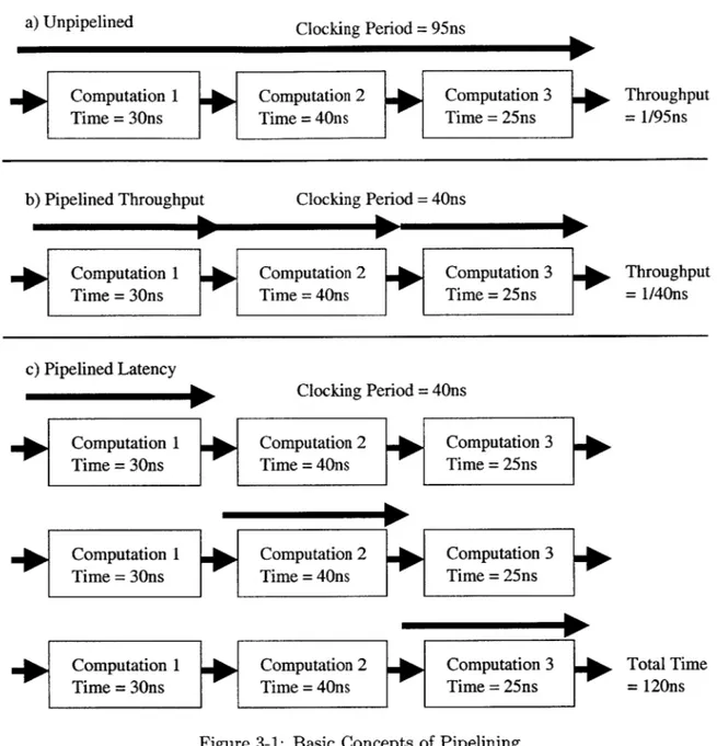
3-1 Basic Concepts of Pipelining . . . . 3-2 A Simple 3D Graphics Pipeline . . . . 3-3 Basic Pipeline Layout on Raw . . . . 3-4 Problems with Simple Sequencing . . . . 4-1 Overview of Implementation . . . . 4-2 State Transition Diagram for a Typical Stage 1 Switch Processor 4-3 The Processor in a System Context . . . .
. . . . 21 . . . . 24 . . . . 28 . . . . 29 . . . . 30 . . . . 37 . . . . 38 . . . . 40 . . . . 47 . . . . 57 . . . . 67 . . . . 71 . . . . 75 . . . . 79 . . . . 80 . . . . 83 . . . . 85 . . . . 86 . . . . 88 Framebuffer Message Header . . . .
Sample Screenshots . . . . Triangle Performance Test Pattern . . . . Performance: Speedup, Utilization, and Estimated Overhead . . Performance: Utilization per Stage . . . . Performance: Active Cycles per Stage . . . . Performance: Triangles and Pixels per Second . . . .
2-1 2-2 2-3 2-4 2-5 5-1 5-2 5-3 5-4 5-5 5-6 5-7
List of Tables
2.1 Coordinate Mapping in Different Texture Modes . . . . 32
3.1 Sequence Numbers Assigned to a Stream of Primitives . . . . 48
4.1 Render State Variables Stored in the First Pipeline Stage . . . . 59
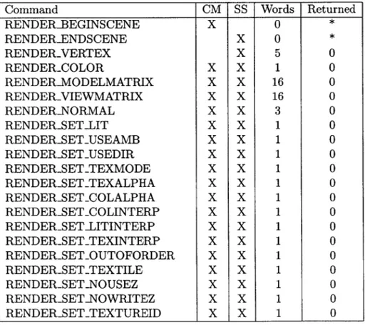
4.2 Rendering Processor Commands . . . . 61
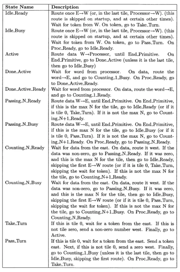
4.3 Full State Transition Table for Stage 1's Switch Code . . . . 66
Chapter 1
Introduction and Motivation
The "Raw" Architecture [21] is a tiled microprocessor array with tightly coupled interpro-cessor networks, programmable static routing, and direct software access to pin I/O. The architecture can be implemented on a single chip, and supports a wide variety of parallel processing paradigms, such as shared memory, message-passing, and systolic array process-ing. A Raw Processor is, at its basic level, an array of microprocessors; however, it can also be configured and treated as a deeply pipelined stream processor [8], a wide-issue processor for instruction-level parallelism [22], or a coarse-grained reconfigurable architecture.
This latter use is of particular interest in this paper, and was one of the original moti-vations for the Raw project. The idea was to create, with Raw, an architecture that could be fine-tuned to different tasks, but which was coarser-grained than FPGAs and therefore on which datapath and other higher-level structures were easier to implement, and perhaps more efficient in terms of performance and space cost, as well.
In this vein, the paper presents an implementation of an architecture for real-time 3D graphics on the Raw processor, hoping that, while not being as efficient as a full-custom design, the processor will attain a large performance improvement over a software-only implementation on a general-purpose CPU. Also, it is hoped that implementing the processor on Raw will prove a much easier engineering task than a full-custom design might be.
A real-time 3D graphics processor is, in general, a co- or slave processor which receives rendering commands from a host processor and outputs a rendered image to a memory known as a "framebuffer." The framebuffer may also be connected to a Video DAC (digital to analog converter) for display on a screen, but this is not strictly necessary. The goal is to offload the chore of rendering 3D images from the main processor so that it may continue to do other useful work, and also to provide a highly optimized datapath for that 3D rendering to attain performance that a general processor would not be able to attain. 3D rendering hardware is used in a wide range of applications, from high-end workstations for scientific and medical imaging to consumer devices such as video game consoles. 3D graphics accelerators have become increasingly popular as consumer-level add-ons to computers, especially for use with video gaming. In this market, the engineering goals include not only high performance, but also low cost and moderate power usage.
The actual process of performing 3D rendering (explained in more detail in Chapter 2) is highly parallelizable due to the typical lack of much dependence between separate parts of a rendered image. Modern graphics processors generally gain large amounts of performance through a combination of pipelining the computation, and running several computations in
parallel. Such a structure might map nicely to a two-dimensional mesh like that of the Raw processor. Additionally, the Raw processor's many modes of communication - streaming messages, dynamic messages, shared-memory - and large amount of I/O bandwidth would prove very useful in a complex multi-featured device such as a 3D rendering processor. For more detail regarding the parallelization of 3D algorithms and how it was applied to the Raw see Chapters 3 and 4.
1.1
Goals
The major goal of this thesis was to design and verify a 3D rendering architecture on a Raw chip from scratch in order to gain insight into the major performance and implemen-tation issues that would come up, especially those specific to the Raw architecture itself. The 3D architecture itself does not need to support state-of-the-art features, but should implement some relatively interesting (if well-known) techniques such as texture mapping, alpha blending, directional lights, and hardware transform and lighting operations. The performance should be reasonable - as in, it should be feasible that the architecture could operate interactively, even if that would require very low resolution or simple scenes. De-tailed performance measurements should be possible, to allow for a good deal of insight into the performance issues that come up. It was hoped that by the end of the project, much more would be known about the bottlenecks and performance pitfalls about implementing such an architecture on Raw, and that this knowledge would be useful to advise future endeavors in the area.
1.2
Methodology
The project described in this thesis was implemented solely as a simulation, although it could conceivably be implemented on existing hardware. A framework was developed around the simulation to be able to verify its correct functionality and to measure detailed information about its performance. Several simple tests were run to verify functionality - not a full test suite by far but enough for reasonable confidence that the device was functioning correctly for the most part. One such test was modified to allow it to run over many different combinations of rendering modes and parameters, and output large batches of performance results to the disk to be analyzed later by scripts. These results were distilled down, and are presented in this thesis along with an intuitive performance model to try to pinpoint where the inefficiencies stemmed from. This information is then used to motivate suggestions for future improvement in similar lines of inquiry.
For more details about the testing methods used in this thesis and their results, see Chapter 5.
1.3
Outline of this Thesis
This thesis begins with a general introduction to 3D rendering algorithms in Chapter 2, both to serve as background information for those not familiar with the topic, and to describe the algorithms used in this project so that the rest of the paper can concentrate on the architectural features of the design. Chapter 3 talks about the design process of trying to parallelize those rendering algorithms on to the Raw, including several hurdles and abandoned ideas along the way. The final design of the rendering architecture as presented
in this thesis is described in detail in Chapter 4. Chapter 5 introduces the verification and performance framework used with the architecture, and presents the performance results along with some discussion. The majority of the discussion, however, is left for Chapter 6, which analyses many ways in which this architecture could be improved upon, and its performance made more competitive with today's technology. Chapter 7 quickly summarizes the thesis.
Additionally, there are several appendices attached to this paper. Appendix A presents some additional rendered images to ease the image clutter in Chapter 5. Appendices B through D present the actual code used to program the Raw, and to build the verification and testing framework. Finally, Appendix E lists the raw data that were used to generate the performance results seen in Chapter 5.
Chapter 2
3D Rendering Algorithms
This chapter serves to introduce the 3D rendering algorithms used by the architecture described in this paper. How these algorithms are parallelized across the Raw chip is described in Chapter 4. The purpose of this chapter is twofold: firstly, as background information on how real-time 3D rendering is generally done, for those readers who may not be very familiar with the subject, and secondly, to describe the specific algorithms used in this project, as a reference for the rest of the paper which assumes this information is known.
As this thesis is intended to study architecture and not algorithms, the actual rendering methods used are relatively standard and simple. Enough rendering features are supported to allow exploration of some non-trivial aspects of the architecture, but many advanced and complex features (which most modern rendering processors support) were not implemented due to the limited time available and scope of the thesis. Namely, features such as bump mapping, environment mapping, programmable shaders, mip-mapping, trilinear filtering, anisotropic filtering, anti-aliasing, and multi-texturing, which have become common on modern graphics cards, were not implemented in this project. However, in the interest of presenting a reasonably usable and interesting rendering pipeline, features such as hardware geometry transform, hardware lighting (supporting one directional hardware light and one ambient), perspective-correct texture mapping (in fact, perspective-correct interpolation of all values), smooth or "Gouraud" shading, hardware z-buffer support, and transparency were implemented, and the algorithms used for these features, among others, are presented here. A good comprehensive source on many aspects of rendering is [11]
Several sources were consulted in the process of writing the rendering algorithms used in this project, primarily the lecture notes available at [3]. and [1].
2.1
Introduction to 3D Rendering in General
3D Rendering is the process of presenting a three-dimensional model as a two-dimensional
image, with correct perspective such that its three-dimensionality is recognizable. More precisely, 3D Rendering is a projection of the three-dimensional model to a two-dimensional plane, and the subsequent rasterization of that projection to a digital image, which is usually displayed on a computer monitor. The projection to a two-dimensional plane may be a perspective projection, in which objects further from the virtual viewer appear smaller, or it may be an orthographic projection, in which objects appear proportional to their original size no matter what distance they are from the viewer.
Real-time 3D Rendering requires that the digital images of a scene be produced very quickly - ideally at least 30 frames per second and typically 60 frames per second and beyond - in order to fool the eye into believing that the scene is in constant motion, and also to allow instantaneous feedback to user controls or other inputs, such as in a video game. Generally, certain methods of 3D Rendering are suitable for real-time rendering while others are not, though the latter may create images of improved quality or realism. For example, ray-tracing [13] is almost exclusively used for non-real-time rendering. 2.1.1 Defining a Scene
When rendering a 3D image, the geometry of the world is generally broken down into sim-pler shapes, known as primitives. With real-time rendering, these primitives are almost exclusively flat triangles, although quadrilaterals are sometimes used as well. Some advan-tages of triangles are that three points uniquely describe a triangle, and that all triangles are guaranteed to fall completely in a plane (which is defined by the same three points as the triangle). Flat surfaces can be easily broken down into patterns of these primitives, and curved surfaces must be approximated as a mesh of primitives. From here on in this paper, it will be assumed that all primitives in the scene are triangles, and the terms "triangle" and "primitive" will be used interchangeably.
Each triangle may have other information associated with it, such as color, texture, light reflectance, transparency, normals (vectors parallel to the original surface of the ob-ject which are used for smoother lighting), and blending mode, to be used in drawing the triangle. More advanced renderers may even support shaders, which are custom programs that determine how to draw each triangle. Additionally, the scene has information asso-ciated with it, such as ambient light and location of lights, position of the camera (which defines the view to be rendered), and so on.
2.1.2 Geometry Transformation
The first step in drawing a scene is to transform the coordinates of the vertices of the trian-gles to coordinates in the two-dimensional image that is to result. In a 3D transformation, straight lines in the scene will always map to straight lines in the final image, and therefore triangles will map to triangles (or polygons to polygons, etc). Actually, this transformation is usually a larger set of transformations each applied consecutively. For example, a scene may contain a model of a desk. That desk model, for the convenience of whomever created the scene, may have its own local coordinate system in which all its primitive vertices are defined. The desk may then be scaled, rotated, translated, and skewed (though desks are rarely askew) to its final position in world coordinates. In fact, it may go even further than this, as there may be a pencil sharpener model on the desk itself, with its own local coor-dinate system. In this case, the pencil sharpener could to be transformed into the desk's coordinate system, and then the desk (plus sharpener) could be transformed into world coordinates. This structure of local coordinate systems for objects, built into compound objects, and finally built into a scene is known as a scene hierarchy
Once all primitives are defined in world coordinates, they are then transformed into the local coordinate system of the viewer, also known as eye space or camera space. In eye space, one axis is generally aligned in the direction that the eye is looking, and the other two specify up-down and left-right directions. For example, the z coordinate may specify distance from the camera, while the y and x coordinates specify up-down and left-right
Image Plane- IaePae
,
~
3D Geometry Eye Point 3D Geometry
Projected' Projected'
Image Image
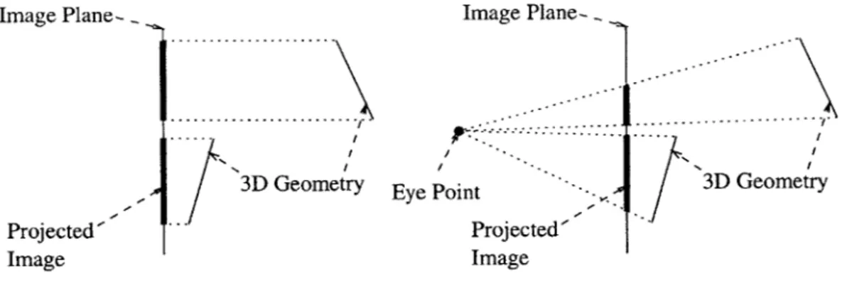
a) Orthographic Projection b) Perspective Projection Figure 2-1: Orthographic vs. Perspective Projection
Figure 2-la shows an orthographic projection, where the depth coordinate is truncated and the geometry appears as a direct projection from the scene to the final image plane.
Figure 2-1b shows the same world geometry with a perspective projection, which causes more distant objects to appear smaller on the image plane. With perspective projection,
there is a virtual "eye point" where all the lines of projection converge.
coordinates respectively.
Next, these three-dimensional coordinates must be projected into two-dimensional co-ordinates for use in the final image. There are several ways to perform this projection. Orthographic projection would simply discard the z coordinate, resulting in a direct projec-tion to the 2D plane. Perspective projecprojec-tion, however, would divide the x and y coordinates by the distance from the viewing plane (which is related to, but not generally the same as
z). This makes distant objects look smaller, creating an image that looks like a realistic two-dimensional representation of a three-dimensional scene. Figure 2-1 illustrates how the scene geometry is projected to the final image plane using orthographic and perspective projection.
Other transformations usually occur, as well. For example, often times the geometry is transformed into a set of coordinates that specifies the visible parts of the scene within a normalized range (such as 0 to 1 or -1 to 1), and any geometry that has coordinates outside that range is partially or fully off the screen (or to close to or too far away from the viewer). These are known as normalized device coordinates, and the range of visible coordinates defines what is known as the viewing frustum. Discarding objects outside of that frustum before further processing is known as culling. Sometimes, objects appear partially within the frustum and must be split up, so that the part outside of the frustum can be culled; this process is called clipping. Generally, culling and clipping is done for performance reasons, although some geometry must be culled for correct operation - most notably, any geometry that has a vertex on the eye point must be culled to avoid a divide by zero error when doing perspective projection, and any geometry behind the image plane usually must be culled to
avoid rendering geometry that appears behind the virtual viewer.
Finally, the coordinate system is transformed to the actual coordinate system of the resulting digital image, where each pixel is addressed by an integer coordinate.
To specify all these transformations, matrices are used, and coordinates expressed as vectors multiplied with matrices result in the new, transformed coordinates. In fact, if several multiplications must happen sequentially, all the matrices for those transformations
Imagie
may be multiplied together to produce one matrix that performs all the transformations in one step. This can result in a large performance gain over doing every transformation individually for every single vertex in the system.
In general, a three-dimensional coordinate can be represented by a column 3-vector, and transformed with a 3x3 matrix, like so:
(
1 0 0[
a d g b eh
c
f
i
\
x y z)
Here are some examples of matrices used for various transforms (adapted from [5]): cos 9 sin 9 0 - sin 9 cos 9 0 0 0 1 A rotation by 9 about the z axis.
I
0
01
cos0 -- sin0 sin9 cos9 A rotation by 9 about the x axis.
sE 0 0 0 sy 0 0 0 sz
Scaling by sx, sy, and sz.
However, this simple matrix multiplication cannot represent all the transformations one would be interested in performing. For example, translations are not representable, and neither are perspective projections. To represent all these transformations, 4x4 matrices are used, along with four-dimensional vectors for the coordinates:
C
a e i m bf
j
n c g k0
d h1
pIC
x y z wThree-dimensional coordinates are represented in the four-dimensional vector by treating w specially - the true values of x, y, and z are obtained by dividing them all by the value of w. Coordinates represented in this way are known as homogeneous coordinates. Most of the time, w = 1, and the rest of the coordinates can be treated normally. Homogeneous coor-dinates are used because now translations and perspective projections of three-dimensional coordinates can be represented in a 4x4 matrix:
1 0 0 t 0 1 0 ty
0
0 1tz
0 0 0 1I
A translation by t , ty, and tz (from [5]).[
1 0 0 0 0 1 0 0 0 0 0 0 1 11
0
0A simple perspective projection, where x and y coor-dinates are divided by the distance z (from [2]).
Generally, if w is nonzero, then the homogeneous coordinates specify a point in space that can be translated, scaled, rotated, etc. However, if w is zero, then the coordinates specify a direction (towards a point at infinity). Directions can be scaled and rotated, but cannot be translated. Normals to surfaces and light directions are two values for which representation as a direction would be appropriate1.
As stated earlier, a large number of transformations can be combined together into one matrix, to speed computation. Generally, geometry is transformed from whatever model space it is in to normalized device coordinates. Then culling occurs, and perspective
divide (where the three coordinates are divided by the value of w). Finally, the resulting coordinates are transformed into pixel addresses for display on the screen (though this can be done by a simple scaling, and does not require a full matrix multiplication). One exception is that normals to surfaces are transformed to world coordinates, rather than directly to normalized device coordinates, for use in lighting calculations (as lights are generally also defined in world coordinates).
2.1.3 Rasterization and Interpolation
Once the image pixel coordinates that correspond to triangle vertices are calculated, then the triangles can be "filled in" with pixels, and this process is called rasterization. One method of performing rasterization is to trace one edge of a triangle, and fill in the rest horizontally from that edge. Another method is to calculate three inequalities, one for each edge, and use them to determine whether a pixel is inside the triangle. Then, for all pixels in a bounding box around the triangle, if it is inside the triangle, draw it.
Along with simply drawing the correct pixels, values from the vertices are interpolated across the triangle. These values can include color, texture coordinates, light intensity, and depth (depth for each pixel is used for depth buffering, described later). Alternatively, each triangle may use the same value for color and light intensity across the entire shape, instead of smoothly interpolating values.
One way to linearly interpolate the values from the three vertices of the triangle is to solve a plane equation of the form v = Ax + By + C, which takes the location on the screen (x, y) and returns an interpolated value at that point, v. The values for A, B and C can be solved for using routine linear algebra using the known solutions at the three vertices of the triangle. Also, to speed things up, instead of calculating the entire formula for every pixel (which requires two multiplies and two adds), one can calculate an initial value for each row of pixels, and an incremental value for the row, which is how much the equation changes for each pixel (O-Ax, where Ax is the spacing between pixels, generally 1). For each pixel in the row, this incremental value is added to the current total, which only requires one addition per pixel.
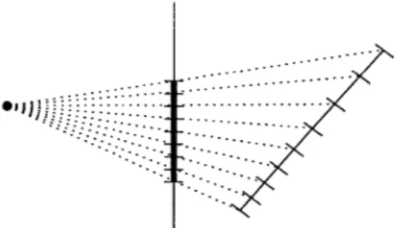
However, unless the primitive is aligned parallel to the image plane, simply interpolating the parameters of the vertices linearly across the screen will not produce accurate results. The reason for this is illustrated in Figure 2-2. Equally spaced points on the screen are spaced further apart on a primitive as it becomes more distant from the viewer, and likewise equally spaced points on the primitive are spaced more closely together on the screen as the primitive becomes more distant. The result is that the parameters, which are assumed to be distributed linearly across the primitive's surface, are distributed in a non-linear fashion on the screen. Interpolating in screen space is usually acceptable for smooth parameters such as color and light intensity, since the inaccuracy will not be easily noticeable. However, with texture coordinates, the resulting textures can easily look incorrect with simple screen-space interpolation, and so-called perspective correct interpolation is generally a must.
To determine how to interpolate variables correctly, recall that in a perspective projec-tion, the coordinates of a vertex in screen space are divided by the distance from the viewer
with a nonzero w. This was simply an oversight, and special logic was needed to make sure normals were not affected by translations.
Figure 2-2: Interpolation in Screen Space
Equally spaced points across the screen result in nonlinearly spaced points across the surface of the primitive, and vice versa. Therefore, interpolating a parameter linearly across the screen will not result in the same values for the pixels as interpolating linearly across the primitive. Interpolating correctly in these situations is called perspective correct
interpolation.
(non-linear interpolation is only required in perspective projections). Before this perspec-tive division, equally spaced coordinates on a triangle's surface can be linearly interpolated across the triangle from its vertices due to the planar nature of a triangle. After the per-spective divide, however, each coordinate on the surface of a triangle must be divided by the distance from the viewer, Z, to produce the equivalent screen coordinate. If x1 and
X2 are the x coordinates of one edge of a triangle before perspective divide, and zi and Z2
are the depths of each of those points respectively, and s is a parameter that is stepped in equally spaced increments from 0 to 1, then a set of undivided x coordinates that are evenly interpolated across the primitive is given by X1 +s(X2 - x1), and a set of screen-space
coordinates that correspond to these undivided x coordinates on the triangle's edge is given by (from [4]):
X1 + s(X2 - X1)
Z1 + s(Z2 - Z1)
However, polygon filling algorithms work the other way: they step linearly across the screen, and need to determine how far along the primitive's surface they have gone for each position on the screen. That is, if x' and x' are (post-perspective-divide) coordinates of the edge
of a triangle in screen-space, which correspond to points x1 and X2 with depths z, and Z2
before perspective divide, and t is a parameter that is stepped in equally spaced increments from 0 to 1 as the rasterizing algorithm is moving across the primitive, then the current screen coordinate that corresponds to t is given by (from [4]):
xi
+tXx'+
- )=+t
(X2 _X1Z1 \Z2 z1
The challenge is to determine a value for s, and hence the distance along the surface of the triangle, for every value of t, which represents the distance along the projected image of the triangle on the image plane. To do this, we set screen coordinates equal to screen coordinates:
x1 + X2 _X1 X1 + s(X2 - X1) zi Z2 Z1 Z1 + s(Z2 - Z1)
and solve for s in terms of t (also from [4]): tzi Z2 + t(zi - Z2)
Now as t is stepped linearly in screen space during rasterization, the corresponding distance along a primitive's surface can be found with the above formula, and the value of s used to interpolate any parameter from one vertex to the other. The resulting interpolated values of the parameter will be perspective correct. This method can be easily extended to two dimensions.
In practice, the above method is rarely used directly, as calculating the formula to map t to s for every pixel is relatively expensive - tzi must be interpolated, which at best requires an addition per pixel for incremental interpolation; then s must be calculated which requires an add and a divide (assuming that the z value in the denominator is incrementally interpolated); and finally the actual parameter must be calculated using vI+s(v2-vi), which requires a multiply and two adds. Instead, parameters at each vertex are pre-multiplied with - as part of the perspective divide step, then are interpolated linearly in screen space, and finally are divided by the screen-space interpolated value of - for that point to produce the interpolated parameter. Assuming incremental interpolations, this method requires two adds and a divide per pixel, in contrast to the 4 adds, one multiply, and one divide required for the straightforward method. This method can be shown to be correct by substituting
for s in vi + S(V2 - vi), to get:
tz (
z2 +
t(zi
- Z2) Manipulating this formula further results in:tl1
VZ
+ Z2(v
2 -vi)
1 1 1)1
V1 -+t - - - +t-V2-t-V11+t
1(Z2 [Z Z1 Z2 Z2 Z1 G2 Z1 1 1 V 1 t 1 1 + t 1 V 2)1
-1 - t-V1 + t- 2)
+t1
1 i - i ) Z1 Z1 ( ZThis is exactly what we are looking for: the value, v, pre-multiplied by 1, linearly interpo-lated in screen space (due to the parameter t), divided by . linearly interpointerpo-lated in screen space. The value v can represent any parameter that is defined at the vertices of the trian-gle that must be interpolated in a perspective-correct manner, such as texture coordinates, color value, light intensity, and so on.
The resulting pixel objects, which contain x and y screen coordinates along with a depth value and interpolated (or perhaps flat-shaded) values of all its parameters, are called fragments. Fragments go through an optional texture lookup, then all their values are blended together to get the final value to be sent to the resulting image, which for the
purposes of this paper is stored in special memory known as the framebuffer.
2.1.4 Rendering to the Framebuffer
When fragments from primitives are drawn to the final buffer that stores the resulting digital image, care must be taken to make sure that closer objects are drawn on top of more distant objects. One method to ensure this is known as the painter's algorithm, in which primitives are first sorted from back-to-front, and then drawn in this order to ensure that closer fragments are overwriting those that are further away, and not vice-versa. However, the painter's algorithm has a hard time dealing with intersecting primitives, and is not very efficient for parallelized rendering schemes, and so a different method is used. This method, known as z-buffering or depth buffering, uses another buffer, separate from the framebuffer, where the current depths of the pixels stored in the framebuffer are kept. When a fragment is to be drawn, first its depth is compared with the pixel already in the framebuffer, by looking up the latter's depth in the z-buffer. If it is in front of that pixel; it is rendered, otherwise it is discarded. Note that even with a z-buffer, translucent primitives must be drawn back-to-front to ensure that they are correctly blending with the polygons behind them, but that opaque polygons can be drawn in any order.
The value stored in the z-buffer is typically not the actual z coordinate of the pixels, but rather a value 1) monotonically related to the depth, so that fragments maintain the correct depth ordering relative to one another, and 2) that when linearly interpolated in screen space provide the same depth ordering as perspective-correct interpolated z values, so that the overhead of perspective-correct interpolation can be avoided in the rasterization stage (see Section 2.1.3). A typical value that could be used in the z-buffer is
(far
+
near) - 2near -fart
far
- nearwhere near and far are the distances of the near and far clipping planes of the viewing frustum, respectively (see Section 2.1.2). The projection matrix can be arranged to auto-matically produce this value for the transformed z' coordinate, after perspective divide.
Using these nonlinearly distributed values instead of z directly also causes the precision of the z-buffer to be much higher closer to the viewer than in the distance, which is usually desirable, depending on the application. When z-buffer precision is not high enough to accurately discern between two very close fragments, then unwanted visual effects can occur. To reduce the likelihood of these effects, the values are stored in the z-buffer with as much numerical precision as possible, usually using 16 or 32-bit fixed point numbers. It is also recommended that the programmer place the near clipping plane as far away from the viewer as possible, and the far clipping plane as close as possible, to make best use of available precision.
This section has introduced the basics on which the 3D rendering algorithms used in this project are based, intended for those without much background on the subject. The
next section details the actual implementation of these algorithms used in this project, for reference use with the rest of this paper, which expands on the parallelization of these
2.2
3D Rendering Implementation of this Project
A single-processor version of the 3D Rendering code used in the processor described in this paper is available in Appendix B. This code is basically a stripped-down version of the fully parallelized code (Appendix C), with code used for parallel synchronization removed and code spread across multiple processors placed into one thread. However, it still retains some elements of the structure of the parallelized code, as it was not written from scratch. The parallelized code and the rendering architecture in general is described in more detail in
Chapters 3 and 4. This section serves to describe the actual 3D rendering algorithms used in the project - to this end, the actual structure of the code and some implementation details are not considered to be very important.
2.2.1 Geometry Transformation
The processor receives from an external source input that is primarily organized by prim-itive, consisting of the coordinates of three vertices to define a triangle, and the texture coordinates for those vertices. The rest of the info that is needed for each vertex (color, normal, texture mode, lighting mode, transparency, etc) is taken from the current render state. The external source can send commands at any time to change the render state, and the new render state will take effect for all subsequent vertices and primitives.
The render state also specifies the transformation matrices that are currently in use - the external controlling program provides a matrix that transforms from the current model coordinates to world coordinates, ModelToWorld, and a matrix that transforms from world coordinates to normalized device coordinates, as well as performing any perspective projection desired, WorldToView. Internally, two more matrices are kept: ModelToView, which is the matrix multiplication of WorldToView and ModelToWorld, and is used to transform incoming geometry directly to normalized device coordinates in one step; and NormalToWorld, which is used specifically to transform vertex normals from model-space to world-space for lighting calculations, and is discussed further below. The WorldToView matrix, after the transformed vector is normalized by dividing all the coordinates by the resulting w value (the fourth coordinate), causes all the x, y, and z coordinates within the viewing frustum to lie in the range -1 to 1. x specifies the horizontal screen coordinate and increases from left to right. y specifies the vertical screen coordinate and increases from top to bottom. z specifies the depth value to be stored in the z-buffer, and therefore should be linearly interpretable as described in Section 2.1.4, and increases from near to far coordinates.
The model-space x, y, z vector is multiplied by the ModelToView matrix, to result in pre-perspective-divide coordinates (this is sometimes known as clipping space). Simple clipping is performed here to remove any geometry that is closer than the near clipping plane, which both removes geometry behind the viewer and vertices that are too close to the eye point. This must occur before perspective divide, as a point too close to the eye point could result in w ~ 0, and a possible divide by zero. Since the perspective divide has not occurred yet, z is compared against ±w instead of +1. Also, the case of w being close to zero is checked for explicitly, in case the transformation matrix is badly formed, or just doing something unexpected.
If a primitive intersects the near clipping plane (rather than being fully on one side or the other), it is simply dropped. Tests against the other planes in the frustum were not implemented due to limited time, although a full implementation would ideally perform
Clipping Plane
a) Original Primitive b) Primitive Split into Three Figure 2-3: Primitives that Intersect the Clipping Plane
Ideally, a primitive that partially intersected a clipping plane would be split into smaller primitives that are either entirely without or outside of the viewing frustum. However, the project described in this paper does not implement this algorithm due to time constraints.
these. Also, a full implementation, instead of dropping a primitive that intersected one of the clipping planes, would instead break the primitive up into smaller primitives, so that each would be fully in or out of the frustum, resulting in a better quality rendering (Figure 2-3). This feature was also not implemented due to time constraints.
At this point, if the primitive is still visible, a quick backface culling check is performed2.
Backface culling removes any polygons that are facing away from the viewer - where in this case having vertices specified in a clockwise order is defined as facing the viewer. Backface culling is done for performance (as most objects are solid, and the sides' backfaces are interior to the object and cannot be seen), and also because the rasterization algorithm used (Section 2.2.2) requires primitives to be oriented in this fashion for it to work correctly. A programmer who desires a double-sided primitive can either render two primitives back to back, or re-arrange vertices in software as necessary.
If the primitive turns out to not be visible at this point, it is discarded and the code moves on to the next primitive. If it is visible, then next up comes the directional and ambient lighting calculations, if lighting is enabled for this primitive. Ambient light's intensity is modulated with the primitive's reflectivity, using a fixed point representation which uses 0-255 to represent 0.0-1.0. The code also uses one global directional light, and the intensity of the light is calculated at every vertex by the negative dot product of the global light direction vector and the "normal" of the vertex. The normal defines a direction perpendicular to the surface of the object at the vertex, and if light is shining directly along the normal it should be brightest, while if it is shining parallel to the surface (at a 90* angle to the normal), it should be darkest. Light shining from the other side of the surface should have no effect (i.e., negative results from the dot product are treated as zero).
The normals for the vertices need to be transformed to world coordinates before they are compared with the light vector, which is also stored in world coordinates. However, there are
2
Actually, it was discovered late in the process that this is implemented incorrectly - backface culling should be performed after perspective division, as the division can re-arrange the vertices and change the primitive's orientation with respect to the viewer. However, this was discovered too late to be able to fix, test, and re-run simulations with the new code, so the older version remains in this paper.
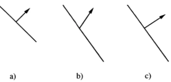
a) b) c) Figure 2-4: Transformation of Normals
Figure 2-4a shows a surface and its normal before translation. Figure 2-4b shows the normal transformed using the same matrix as the geometry, which results in a skewed image. Figure 2-4c shows a correctly transformed normal under the same geometry
transformation.
two things one must be careful of when transforming normals: 1) that normals should not be translated, and 2) that under certain transformations, the normal cannot be transformed to world coordinates by the same matrix that is used for the geometry vertices. The code creates a special transformation matrix to be used on normals called NormalToWorld, using the function MatrixInvTrans. This function ensures the former consideration by only using the upper 3x3 part of the matrix, which results in no translation. The latter problem is illustrated in Figure 2-4. To correctly transform a normal under all circumstances, one must use the transpose of the inverse of the geometry-to-world transformation matrix. However, the scaling of the normal is not important, as it is normalized after it is transformed; therefore, only the adjoint needs to be calculated instead of the full inverse (which is the adjoint divided by the determinant). The code to do this calculation is from [11]. Given the input matrix M, the transposed adjoint is:
mllm 22 - m 12m 2 1 m 1 2m 2O - mlOm 22 mIOm21 - m1 1m 20 0 m21mO2 - m22mOl m2 2mOO - m20mO2 m20mOl - m2 1mOO 0 molm12 - m02m1 1 m02m10 - moom12 mOm 1 1 - m0 1m1 0 0
0 0 0 1]
Finally, the vertices' new coordinates x', y', and z', the color and alpha values r, g, b, and a, the texture coordinates u and v, and the light intensity intensity are all multiplied by }, if applicable. i is also stored as wi, and all these values, along with mode information, are sent to Stage 2, which performs rasterization and interpolation.
2.2.2 Rasterization and Interpolation
To rasterize the triangle, the code first calculates a bounding box around the triangle using the min and max coordinates of its vertices. Then it sets up the incremental interpolation for each parameter that is to be interpolated, scans across the entire bounding box region, and for every pixel within the polygon, sends an "Untextured Fragment" to the next stage, along with its interpreted parameters.
Before the triangle is rasterized, however, the final transformation step is performed: transforming from normalized coordinates to screen pixel coordinates, where the pixel coor-dinates run from 0 to VWIDTH and VHEIGHT, which are defined at compile time. Vertex coordinates are defined as floating point numbers, where 0 is the left or top screen edge,
0.25 1.875 3.25 0 0- - -- -- - -- - 0.25 0.5 - - 1.5---2.5 - -2.675 3.5- --4 ---...-.-- .. 3.875 0 4 0.5 1.5 2.5 3.5
Figure 2-5: riangle Rasterization to Pixels
The dotted grid represents the actual screen pixels, with the black dots in the center of each square representing the center of the pixel. The coordinates to the left and bottom are screen-space coordinates. A triangle to be rendered has heavy dashed lines, and dots for its vertices, with its vertex coordinates given above and to the right of the image. The
black rectangle represents the initial bounding box used for rasterization of the triangle, and the shaded pixels are those which are actually generated once rasterization is
complete.
and VWIDTH + 1 and VHEIGHT + 1 are the right and bottom edges, respectively. Pixels are centered on .5 values - 0.5, 1.5, 2.5, etc., up to VWIDTH + 0.5 or VHEIGHT + 0.5. In this system, a floating point value can simply be truncated to give you its nearest screen pixel neighbor. When rasterizing, a pixel is only filled in if its center point is within the primitive - therefore, the actual bounding box need only include those pixels whose centers are within the primitive's general (floating point) bounding box. An example triangle on a small grid of pixels is shown in Figure 2-5, with the bounding box shown, and pixels within the primitive shaded grey.
Next, the stage sets up the equations for each line of the primitive, as well as each variable that is to be interpolated (see Section 2.1.3). To determine whether a pixel is within the triangle, three plane equations are set up, one for each line, that evaluate to less than or equal to zero if the pixel is on the "inside" side of the line, or on the line, and greater than zero if the pixel is on the "outside" side of the line. The sides are determined by assuming that the triangle vertices are given in a clockwise ordering. If any pixel evaluates all three line equations to less than or equal to zero, then it is inside the triangle and a fragment is generated. Given line vertices (x1, yi) and (x2, y2), the equation for each line is:
1 = ax
+
by + c a = Y2 -Yi
C = y1X2 - Y2Xl
where 1 < 0 means the pixel (x, y) is on the right-hand side of the line going from (x1, yi) to (x2, Y2), which is the inside of the triangle made up of three of such lines defined in a clockwise order.
The set-up of equations to interpolate the vertex parameters is the same for each pa-rameter to be interpolated (color r, g, b, alpha a, texture coordinates u and v, depth z', light intensity i, and perspective correction factor 1). The generic parameter p, along with the parameter's values at each of the vertices, po, p1, and P2, where the vertices themselves have coordinates (x0, yo), (xI, yi), and (x2, Y2), will be used in place of the above variables to demonstrate the form of the set-up equations:
P = Pax+ PbY + Pc
1
Pa = (PO(Y1 -Y2) - YO(PI - P2) + be)
det M 1
Pb = (xO(PI - P2) - P0(x1 - x2) + b2e) det M
1
Pc
= det M (Pome - x0bie - yob2e) 1 _1det M x0(y1 -y2) - Y0(X1 - X2) + me
me = Xly2 - X2Y1 bie = P1Y2 - P2Y1
b2e = X1P2 - X2P1
The det M, me, bie, and b2e variables are calculated separately as they are used in more than one location, and calculating them once saves set-up time3.
When stepping through the bounding box to perform the rasterization, the equations for the triangle's lines and for each of the parameters are evaluated incrementally. The initial value for each row is calculated, as well as an incremental amount that is added to the value for each pixel traversed. Since all the equations are linear, this generates a very accurate solution very quickly (one add per pixel). In the case of generic parameter p, the incremental value is RAx, where Ax is the spacing between pixels, and with a pixel spacing of 1, this ends up being simply pa (which would be called "pdx" in the code). The starting value of each row is also generated incrementally from the starting value of the previous row, by adding 2Ay, which is simply Pb, or "pdy" in the code. One final optimization performed is that when pixels within the triangle are found in a row, the loop ends as soon as another pixel outside of the triangle is found, instead of always going to the end of the bounding box.
One exception is that the z values are calculated from the full equations each time instead of via incremental evaluation. They are also stored in a fixed point representation from this point forward. Both of these are to help increase the dynamic range of the z-buffer - however, the current implementation of this code does not take full advantage of
3
Note that there may be vastly more efficient ways to perform these same calculations, and all the calculations in this project. This project was mostly concerned about generating a correct and reasonably fast implementation, so not as much time was spent on trying to optimize it as much as possible, nor research the best possible algorithms for the job
Texture Coordinates
Original -1.4 -1.2 -1.0 -0.8 -0.6 -0.4 -0.2 0.0 0.2 0.4 0.6 0.8 1.0 1.2 1.4 1.6 1.8 2.0 2.2
Repeat 0.6 0.8 0.0 0.2 0.4 0.6 0.8 0.0 0.2 0.4 0.6 0.8 0.0 0.2 0.4 0.6 0.8 0.0 0.2
Mirror 0.6 0.8 1.0 0.8 0.6 0.4 0.2 0.0 0.2 0.4 0.6 0.8 1.0 0.8 0.6 0.4 0.2 0.0 0.2
Clamp 0.0 0.0 0.0 0.0 0.0 0.0 0.0 0.0 0.2 0.4 0.6 0.8 1.0 1.0 1.0 1.0 1.0 1.0 1.0 Table 2.1: Coordinate Mapping in Different Texture Modes
This table shows how the original texture coordinates for each fragment get mapped into a 0-1 range for texture lookup. Repeat repeats the same texture over and over in either direction; Mirror does the same but flips every other instance of the texture; and Clamp sets the coordinate to the closest edge of the 0-1 range (actually, Clamp uses the color of
the last texel on either edge instead of 0.0 and 1.0 exactly, which have different interpretations when used under bilinear filtering).
the range available with the fixed point notation, as the calculation still occurs with 32-bit floating point numbers.
Each untextured fragment generated by this algorithm is passed then to Stage3, where texturing and blending occur.
2.2.3 Texture Mapping and Blending
At this point, the fragment's texture value is looked up if necessary, and the final color value and alpha of the fragment is determined from the texture value, the light intensity, the color value, and its blending modes.
Texture coordinates are defined as floating point values from 0 to 1, where 0 is the left or top edge of the texture, and 1 is the bottom or right edge. Just like with screen coordinates, the texture pixels' (or texels') centers fall on 0.5, 1.5, 2.5, etc. Values less than 0 and greater than 1 are allowed, and they are interpreted according to the primitive's wrapping mode: none, repeat, mirror, and clamp. A wrapping mode of "none" means that texels outside of the 0-1 range should be left black. "Repeat" means that the texture should be treated as an infinite tiled array, such that a coordinate of 1.3 should be treated as 0.3, 4.6 should be treated as 0.6 and -3.9 should be treated as 0.1. "Mirror" is similar to repeat, except that alternating tiles are flipped, so that adjacent tiles are mirrors of one another. "Clamp" simply takes the texel value of the closest actual texture edge (0 or 1) and uses that value forever in either direction. Table 2.1 demonstrates the mapping of coordinates in different texture modes.
The normalized texture coordinates are then multiplied by the width or height of the texture to generate texel coordinates - these coordinates are simply truncated in nearest-neighbor mode, which produces a blocky-looking texture but renders more quickly. Also available is bilinear filtering, which interpolates linearly between texel colors to create a smoother appearance (it is called bilinear because the interpolation occurs on a two-dimensional texture). For bilinear filtering, the colors of the four texels that surround the given point are retrieved from memory, and the final color is a weighted average of the texels according to the given point's distance from their texture centers. To make this easier, the code shifts everything by 0.5, so that pixel centers are aligned with integers, and then the actual texel coordinates are compared with the truncated coordinates, and the truncated coordinates plus one. Special care must be taken so that the Repeat, Mirror, and Clamping modes work correctly under bilinear filtering, by re-wrapping after the shift occurs, and