Data-Driven Methods for Statistical Verification of
Uncertain Nonlinear Systems
by
John Francis Quindlen
M.S., The Pennsylvania State University (2012)
B.S.,The Pennsylvania State University (2010)
Submitted to the Department of Aeronautics and Astronautics
in partial fulfillment of the requirements for the degree of
Doctor of Philosophy
at the
MASSACHUSETTS INSTITUTE OF TECHNOLOGY
February 2018
c
○
Massachusetts Institute of Technology 2018. All rights reserved.
Author . . . .
Department of Aeronautics and Astronautics
December 13, 2017
Certified by. . . .
Jonathan P. How
R. C. Maclaurin Professor of Aeronautics and Astronautics
Thesis Supervisor
Certified by. . . .
Ufuk Topcu
Assistant Professor of Aerospace Engineering and Engineering
Mechanics
Certified by. . . .
Girish Chowdhary
Assistant Professor of Agricultural and Biological Engineering
Certified by. . . .
Russ Tedrake
Toyota Professor of Electrical Engineering and Computer Science
Accepted by . . . .
Hamsa Balakrishnan
Associate Professor of Aeronautics and Astronautics
Chair, Graduate Program Committee
Data-Driven Methods for Statistical Verification of
Uncertain Nonlinear Systems
by
John Francis Quindlen
Submitted to the Department of Aeronautics and Astronautics on December 13, 2017, in partial fulfillment of the
requirements for the degree of Doctor of Philosophy
Abstract
Due to the increasing complexity of autonomous, adaptive, and nonlinear systems, engineers commonly rely upon statistical techniques to verify that the closed-loop sys-tem satisfies specified performance requirements at all possible operating conditions. However, these techniques require a large number of simulations or experiments to ex-haustively search the set of possible parametric uncertainties for conditions that lead to failure. This work focuses on resource-constrained applications, such as prelimi-nary control system design or experimental testing, which cannot rely upon exhaustive search to analyze the robustness of the closed-loop system to those requirements.
This thesis develops novel statistical verification frameworks that combine data-driven statistical learning techniques and control system verification. First, two frameworks are introduced for verification of deterministic systems with binary and non-binary evaluations of each trajectory’s robustness. These frameworks implement machine learning models to learn and predict the satisfaction of the requirements over the entire set of possible parameters from a small set of simulations or experiments. In order to maximize prediction accuracy, closed-loop verification techniques are devel-oped to iteratively select parameter settings for subsequent tests according to their expected improvement of the predictions. Second, extensions of the deterministic verification frameworks redevelop these procedures for stochastic systems and these new stochastic frameworks achieve similar improvements. Lastly, the thesis details a method for transferring information between simulators or from simulators to exper-iments. Moreover, this method is introduced as part of a new failure-adverse closed-loop verification framework, which is shown to successfully minimize the number of failures during experimental verification without undue conservativeness. Ultimately, these data-driven verification frameworks provide principled approaches for efficient verification of nonlinear systems at all stages in the control system development cycle. Thesis Supervisor: Jonathan P. How
Acknowledgments
The past few years have been an interesting and enlightening phase of my life. My time at MIT has introduced me to countless new concepts and ideas that will serve me well in the future and has cultivated my professional development. It’s been quite a journey and I’d like to acknowledge the following people for their help and support along the way.
First, I would like to thank my advisor, Professor Jonathan How for his guidance and wisdom. Throughout the years, I was always amazed by his ability to remember the smallest of details from our previous conversations and his breadth of knowledge about all things “control.” His inputs would often highlight previously unknown limitations of existing work and help me solidify and buttress the contributions of my research. Through his guidance, I was able to become a significantly better researcher and ask the right questions about a problem.
I would also like to thank my thesis committee, Professors Girish Chowdhary, Ufuk Topcu, and Russ Tedrake, for their invaluable input and support. I’ve worked with Girish since my first days in ACL and have greatly benefited from his continued advice over the past years. Unbeknown to me at the time, my earliest conversations with Ufuk were some of the most critical as they ultimately led me down the direction taken in this thesis. He helped me understand the strengths and weaknesses of the various analytical and statistical verification techniques and their implementation. I would also like to thank Russ for his help in narrowing down my thesis topic and connecting it to the wider class of applications.
I am very grateful to my thesis readers, Dr. Nghia Trong and Dr. Stefan Bieni-awski, for their help in the last stages of this thesis. Nghia has not been at MIT long, but already I’ve picked his brain about all things active learning and statistical inference. Likewise, Stefan was a fantastic supervisor during my internship at Boeing and that experience also directly motivated this thesis research. Myself and this work have continued to benefit from his insights on industry’s challenges and procedures with respect to flight control system design and verification.
Without my labmates and friends, I would never have made it to this point. I would like to thank my labmates past and present - Brett Lopez, Steven Chen, Justin Miller, Mark Cutler, Shayegan Omidshafiei, Mike Everett, Kris Frey, and everyone else - for their collaboration on psets, advice on research, funny banter, and helping me stay grounded. They made our office space as enjoyable as possible, especially during all those late nights and weekends. I’m glad to have my friends Tony Tao, Matt Keffalas, Jess Hebert, and Andrew Owens for their support here at MIT. I appreciate all those Friday nights where we would unwind and watch movies or play games after a long week. The same goes for my old roommates Bobby Klein and David Clifton. I also need to thank my friends from Penn State who are up in the greater Boston area: Alan Campbell, Andrew Weinert, Charlie Cimet, and Pei Wang. I would have never guessed we would still be living in the same area after our time in undergrad. I also can’t forget my best friends scattered across the country: Joe Wood, Matt Sowa, and Henry Ball. All these friends got me through the up and downs of grad school (and there were many downs).
Finally, I would like to thank my family for all their unending support. My parents have always encouraged me to pursue my passions, whatever they were, and worked tirelessly for my sister and I. There is no way I would be in my current position without them and I am eternally grateful.
Contents
1 Introduction 21 1.1 Motivation . . . 22 1.2 Problem Statement . . . 26 1.2.1 Challenges . . . 26 1.3 Literature Review . . . 281.3.1 Analytical Verification Methods . . . 28
1.3.2 Statistical Verification Methods . . . 30
1.4 Summary of Contributions . . . 33
2 Background 37 2.1 Support Vector Machines . . . 37
2.1.1 Linear Classifiers . . . 38
2.1.2 Nonlinear Classifiers . . . 38
2.2 Gaussian Process Regression Models . . . 41
2.2.1 Training . . . 42
2.2.2 Predictions . . . 44
2.2.3 Hyperparameter Optimization . . . 46
2.3 Temporal Logic . . . 48
3 Deterministic Verification with Binary Evaluations of Performance 51 3.1 Problem Description . . . 51
3.1.1 Discrete Evaluations of Performance Requirement Satisfaction 54 3.1.2 Region of Satisfaction . . . 55
3.2 Deductive Verification Methods . . . 56
3.2.1 Limitations . . . 58
3.3 Statistical Data-Driven Verification . . . 60
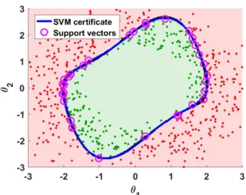
3.3.1 SVM Classification Models . . . 60
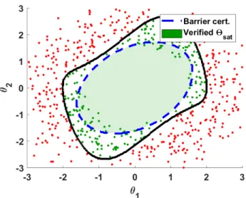
3.3.2 Comparison to Simulation-Guided Barrier Certificates . . . 65
3.4 Closed-Loop Statistical Verification . . . 66
3.4.1 Sample-Selection Criteria . . . 68
3.4.2 Sequential Sampling . . . 70
3.4.3 Batch Sampling . . . 72
3.5 Simulation Results . . . 76
3.5.1 Van der Pol Oscillator . . . 76
3.5.2 Concurrent Learning Model Reference Adaptive Controller . . 81
3.5.3 Adaptive System with Control Saturation . . . 85
3.6 Summary . . . 88
4 Deterministic Verification with Improved Evaluations of Trajectory Robustness 89 4.1 Problem Description . . . 90
4.1.1 Continuous Measurements of Performance Requirement Satis-faction . . . 90
4.2 Regression-based Binary Verification . . . 93
4.2.1 Gaussian Process Regression Model . . . 94
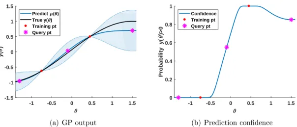
4.2.2 Prediction Confidence . . . 98
4.3 Closed-Loop Statistical Verification . . . 100
4.3.1 Sample-Selection Criteria . . . 101
4.3.2 Sequential Sampling . . . 107
4.3.3 Batch Sampling . . . 109
4.4 Simulation Results . . . 116
4.4.1 Concurrent Learning Model Reference Adaptive Controller . . 117
4.4.3 Adaptive Control with Complex Temporal Specifications . . . 127
4.4.4 Lateral-Directional Autopilot . . . 131
4.5 Summary . . . 134
5 Stochastic Verification with Gaussian Distributions of Trajectory Robustness 137 5.1 Problem Description . . . 138
5.1.1 Distribution of Trajectory Robustness Measurements . . . 140
5.1.2 Satisfaction Probability Function . . . 143
5.2 Regression-based Stochastic Verification . . . 145
5.2.1 Gaussian Process Regression Model . . . 145
5.2.2 Measuring Prediction Accuracy . . . 149
5.3 Closed-Loop Statistical Verification . . . 152
5.3.1 Sample-Selection Criteria . . . 153
5.3.2 Sampling Algorithms . . . 160
5.4 Extension: Heteroscedastic Gaussian Distributions . . . 163
5.4.1 Heteroscedastic Gaussian Process Regression Model . . . 166
5.4.2 Modifications to the Stochastic Verification Framework . . . . 169
5.5 Discussion: Non-Gaussian Distributions . . . 171
5.6 Simulation Results . . . 173
5.6.1 Concurrent Learning Model Reference Adaptive Controller . . 173
5.6.2 Robust Multi-Agent Task Allocation . . . 186
5.6.3 Lateral-Directional Autopilot . . . 189
5.7 Summary . . . 194
6 Extension: Stochastic Verification with Bernoulli Evaluations of Per-formance 197 6.1 Problem Description . . . 198
6.2 Probabilistic Classifiers for Stochastic Verification . . . 201
6.2.1 Expectation Propagation Gaussian Process Models . . . 202
6.3 Simulation Results . . . 206
6.3.1 Concurrent Learning Model Reference Adaptive Controller . . 208
6.3.2 Stochastic Van der Pol Oscillator . . . 211
6.4 Summary . . . 216
7 Multi-Stage Verification and Experimental Testing 217 7.1 Forward Transfer in Multi-Stage Verification . . . 218
7.1.1 Forward Transfer with Nonzero Priors . . . 219
7.2 Impact of Failures in Experimental Testing . . . 224
7.2.1 Region of Safe Operation . . . 225
7.2.2 Problem with Trajectory Robustness Measurements . . . 227
7.3 Failure-Adverse Closed-Loop Verification . . . 229
7.3.1 Forward Transfer of Simulation-Based Predictions . . . 230
7.3.2 Selection Criteria . . . 233
7.3.3 Sampling Algorithms . . . 236
7.4 Demonstration of Failure-Constrained Verification . . . 240
7.5 Summary . . . 246
8 Conclusions and Future Work 249 8.1 Future Work . . . 251
A Concurrent Learning Model Reference Adaptive Control 257
B Robust Multi-Agent Task Allocation for Aerial Forest Firefighting 263
C Lateral-Directional Autopilot Model 269
List of Figures
1-1 Crash of the NASA Helios aircraft . . . 24 1-2 Verification as a step within a broader control system design process . 25 3-1 Illustration of simulation-guided barrier certificates on a Van der Pol
oscillator . . . 58 3-2 Lyapunov function-based predicted region of satisfaction for a Van der
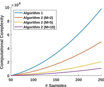
Pol oscillator . . . 59 3-3 SVM-based predicted region of satisfaction for a Van der Pol oscillator 66 3-4 Computational complexity of the sequential and batch closed-loop
ver-ification procedures for binary measurements . . . 76 3-5 Example 3.5.1: Ranking of prospective sample locations for the VDP
example . . . 78 3-6 Example 3.5.1: Sample selections for different batch sizes . . . 79 3-7 Example 3.5.1: SVM-based prediction model after 250 samples . . . . 79 3-8 Example 3.5.1: Misclassification error convergence of statistical
verifi-cation techniques . . . 80 3-9 Example 3.5.1: Estimation error for online validation methods . . . . 82 3-10 Example 3.5.2: Ranking of prospective sample locations . . . 83 3-11 Example 3.5.2: Prediction model and misclassification error convergence 84 3-12 Example 3.5.2: Estimation error for online validation methods . . . . 85 3-13 Example 3.5.2: Effect of increasing false-positive penalties . . . 86 3-14 Example 3.5.3: Total misclassification error convergence . . . 88
4-1 Comparison of two trajectories with the same binary evaluation but different continuous measurements . . . 92 4-2 Illustration of prediction confidence for GP-based deterministic
verifi-cation . . . 100 4-3 Binary classification entropy as a function of prediction confidence . . 104 4-4 Computational complexity of the sequential and batch closed-loop
ver-ification procedures for non-binary measurements . . . 116 4-5 Comparison of the chosen samples for the different batch sampling
techniques . . . 117 4-6 Example 4.4.1: Regression surface corresponding to the actual
satis-faction of the performance requirement over Θ . . . 119 4-7 Example 4.4.1: Initial prediction model after an initial training dataset
of 50 trajectories . . . 120 4-8 Example 4.4.1: Final prediction model after 350 samples . . . 120 4-9 Example 4.4.1: Misclassification error convergence of Algorithm 6 in
comparison to the other approaches . . . 121 4-10 Example 4.4.1: Ratio of runs where Algorithm 6 directly outperforms
the competing approaches . . . 123 4-11 Example 4.4.1: Illustration of confidence levels in the predictions . . . 124 4-12 Example 4.4.1: Rate of misclassification error in the 95% prediction
confidence level . . . 124 4-13 Example 4.4.1: Average misclassification error of the closed-loop
pro-cedures with and without hyperparameter optimization . . . 126 4-14 Example 4.4.2: Rate of misclassification errors for Algorithm 3 and the
competing approaches . . . 128 4-15 Example 4.4.2: Ratio of runs where Algorithm 3 directly outperforms
the competing approaches . . . 128 4-16 Example 4.4.3: Misclassification error convergence of Algorithm 6 in
4-17 Example 4.4.3: Ratio of runs where Algorithm 6 directly outperforms the competing approaches . . . 130 4-18 Example 4.4.3: Rate of misclassification error in the 95% prediction
confidence level . . . 131 4-19 Example 4.4.4: Misclassification error convergence of Algorithm 6 in
comparison to the other approaches . . . 134 4-20 Example 4.4.4: Ratio of runs where Algorithm 6 directly outperforms
the competing approaches . . . 134 4-21 Example 4.4.4: Rate of misclassification error in the 95% prediction
confidence level . . . 135 5-1 Illustration of the effects of stochasticity in the closed-loop trajectory 140 5-2 Distribution of robustness measurements for trajectories with the same
initialization . . . 142 5-3 Illustration of the satisfaction probability function as the cumulative
distribution of the Gaussian PDF . . . 144 5-4 Illustration of prediction error resulting from uncertainty over the mean
of the distribution . . . 150 5-5 Approximation of CDF variance using the 1st order Taylor series
ex-pansion . . . 152 5-6 Binary classification entropy fails to quantify prediction uncertainty in
stochastic systems . . . 155 5-7 Comparison of homoscedastic and heteroscedastic Gaussian distributions165 5-8 Example 5.6.1: Histogram of robustness measurements from 500
re-peated trajectories at the same parameter setting . . . 174 5-9 Example 5.6.1: True satisfaction probability function for the stochastic
CL-MRAC system . . . 176 5-10 Example 5.6.1: Deterministic measurements from Example 4.4.1 for
comparison to the mean of the noisy measurements in this stochastic variation on the problem . . . 176
5-11 Example 5.6.1: Predicted satisfaction probability function at the initial training step . . . 177 5-12 Example 5.6.1: Illustration of the CDF variance selection criterion and
the chosen set of future training locations . . . 178 5-13 Example 5.6.1: Predicted satisfaction probability function halfway through
the verification process after 250 trajectories . . . 179 5-14 Example 5.6.1: Predicted satisfaction probability function at the end
of the verification after all 450 trajectories . . . 179 5-15 Example 5.6.1: Mean absolute error convergence of Algorithm 8 in
comparison to the other sampling strategies . . . 180 5-16 Example 5.6.1: Mean absolute error convergence with static
hyperpa-rameters . . . 180 5-17 Example 5.6.1: Ratio of runs where Algorithm 8 directly outperforms
the competing sampling strategies . . . 181 5-18 Example 5.6.1: Concentration of prediction error in points with the
top 1% of CDF variance . . . 183 5-19 Example 5.6.1: Concentration of prediction error in points with the
top 5% of CDF variance . . . 183 5-20 Example 5.6.1: Changes in the probability of requirement satisfaction
associated with increases and decreases in process noise . . . 184 5-21 Example 5.6.1: Mean absolute error convergence with lower process noise185 5-22 Example 5.6.1: Mean absolute error convergence with higher process
noise . . . 185 5-23 Example 5.6.2: Mean absolute error performance with low
measure-ment variance . . . 187 5-24 Example 5.6.2: Mean absolute error performance with high
measure-ment variance . . . 187 5-25 Example 5.6.2: Concentration of prediction error in points with the
5-26 Example 5.6.2: Concentration of prediction error in points with the top 5% of CDF variance . . . 188 5-27 Example 5.6.3: Comparison of mean absolute error convergence
as-suming the standard measurement distribution . . . 190 5-28 Example 5.6.3: Comparison of mean absolute error convergence after
the requirement is loosened by 10 feet . . . 191 5-29 Example 5.6.3: Comparison of mean absolute error convergence after
the requirement is loosened by 20 feet . . . 191 5-30 Example 5.6.3: Concentration of prediction error in points with the
top 1-5% of CDF variance . . . 192 5-31 Example 5.6.3: Changes in variance across the set of all operating
conditions as the result of a heteroscedastic Gaussian distribution . . 193 5-32 Example 5.6.3: Degradation in mean absolute error if the baseline GP
is applied to a heteroscedastic distribution. . . 194 5-33 Example 5.6.3: Comparison of mean absolute error convergence using
homoscedastic vs. heteroscedastic GP models. . . 195 6-1 Binomial distributions for empirical estimation of the probability of
requirement satisfaction at a particular parameter setting . . . 201 6-2 Example 6.3.1: True probability of requirement satisfaction for the
stochastic CL-MRAC system . . . 209 6-3 Example 6.3.1: Predicted satisfaction probability function at the initial
training step and after 20 iterations of Algorithm 11. . . 209 6-4 Example 6.3.1: Comparison of mean absolute error convergence for the
different sampling strategies . . . 210 6-5 Example 6.3.1: Ratio of runs where Algorithms 10 and 11 directly
outperform or match the MAE levels of the other sampling approaches. 211 6-6 Example 6.3.2: True probability of requirement satisfaction for the
6-7 Example 6.3.2: Predicted satisfaction probability function at the initial training step and after 20 iterations of Algorithm 11. . . 213 6-8 Example 6.3.2: Comparison of mean absolute error convergence for the
different sampling strategies . . . 214 6-9 Example 6.3.2: Ratio of runs where Algorithms 10 and 11 directly
outperform or match the MAE level of the other sampling approaches. 214 6-10 Example 6.3.2: True probability of satisfaction with higher variance . 215 6-11 Example 6.3.2: Comparison of mean absolute error convergence for the
different sampling strategies for the high variance case. . . 215 7-1 Illustration of zero- and nonzero-mean priors . . . 222 7-2 Example of a safety requirement for an aircraft with unequal costs of
satisfactory and unsatisfactory trajectories . . . 225 7-3 Illustration of the region of safe operation . . . 226 7-4 Selection of the most robust point according to the simulation predictions.232 7-5 Example 7.4: True probability of satisfaction and safe operating region
for the simulation stage . . . 242 7-6 Example 7.4: True probability of satisfaction and safe operating region
for the real-world dynamics . . . 242 7-7 Example 7.4: Comparison of prediction error convergence and the
num-ber of failures using the previous active sampling approaches . . . 244 7-8 Example 7.4: Illustration of the effects of small number of failures
upon the prediction accuracy when using the previous active sampling approaches . . . 244 7-9 Example 7.4: Evolution of the predicted region of safe operation with
each additional experiment . . . 245 7-10 Example 7.4: Comparison of a batch version of Algorithm 12 against
7-11 Example 7.4: Comparison of a batch version of Algorithm 12 against the previous active sampling approaches modified with a restricted search area . . . 247 7-12 Example 7.4: Comparison of sequential Algorithm 12 against the
pre-vious active sampling approaches modified with a restricted search area 247 B-1 Illustration of realized mission score as a function of wind parameters 266 C-1 Components of the lateral-directional autopilot and flight control
sys-tem for the de Havilland Beaver flight simulation model . . . 270 C-2 Satisfaction of the heading autopilot’s requirements over an example
List of Tables
3.1 Comparison of SVM and barrier certificate prediction accuracy for a Van der Pol oscillator . . . 66
Chapter 1
Introduction
Control systems are employed to ensure an open-loop system adequately satisfies a set of performance objectives. For instance, possible open-loop plants under consid-eration may range from localized subsystems like a computer hard-drive to physical vehicles such as an aircraft or automobile, or even higher-level system-of-systems like a team of interacting robotic agents. All of these applications will typically require some form of control system and more complex systems-of-systems will include mul-tiple layers of control.
As the demand for higher performance, efficiency, and autonomy grows, advanced control techniques will be increasingly relied upon to meet these demands. Complex methods such as model reference adaptive control (MRAC) [1], reinforcement learn-ing [2], and a variety of other robust nonlinear control architectures [3] will replace traditional linear control techniques which simply cannot meet the demands. These advanced control approaches have already experimentally demonstrated the ability to control damaged aircraft [4–6], aerobatic helicopters [7–9], and drifting racecars [10], and have been proposed as key enablers for brand new applications such as hyper-sonic [11] and lightweight flexible aircraft [12,13].
The largest obstacle impeding wider acceptance and implementation of advanced control techniques is the lack of trust in the robustness of the closed-loop system. The complexity and nonlinearity of the control architectures which allow them to perform so well also complicates predictive analysis of the closed-loop system’s trajectory. For
instance, reinforcement learning will eventually converge towards a locally-optimal controller, but there is no guarantee an intermediate controller will not cause catas-trophic failure let alone satisfy the performance requirements. The difficulty in ana-lyzing the robustness is further compounded by the fact the systems of interest are usually expected to operate over a wide range of possible conditions with little-to-no human oversight. Given the various conditions and nonlinear evolution of the states, it is extremely difficult to guarantee all the possible trajectories will meet the objec-tives. Until the approach is shown to either work robustly or gracefully degrade, any new control architecture is of rather limited utility even if experimental results point to large potential improvements. In fact, the Office of the US Air Force Chief Scien-tist [14] recently stated that “establishing certifiable trust in autonomous systems is the single greatest technical barrier that must be overcome to obtain the capability advantages that are achievable by the increasing use of autonomous systems” and “this level of autonomy will be enabled only when automated methods for verification and validation of complex, adaptive, highly nonlinear systems are developed.” This thesis develops data-driven, black-box methods for statistical verification of nonlinear systems without the need for human supervision or restrictive modeling assumptions. The chapters will demonstrate these new verification techniques on multiple examples with adaptive, nonlinear, or otherwise complex control systems.
1.1 Motivation
The fundamental goal of control system verification is to identify at which operating conditions the closed-loop system will satisfy a certain set of performance require-ments and at which conditions it will not. These requirerequire-ments may cover a wide range of possible criteria such as simple concepts like stability and boundedness of the states to more complex functions of state and time. These well-defined requirements are provided by relevant certification experts or authorities, such as military [15] and civilian [16] aviation agencies. Regardless of the exact specifics, the closed-loop sys-tem must successfully meet all the given requirements in order for the control syssys-tem
to be considered “satisfactory” for final implementation.
There are multiple approaches that can be taken towards verification, but they typically fall into two general categories: deductive analytical techniques and statis-tical methods. Analystatis-tical verification approaches encompass proof-based certificates or numerically-exact solutions which provably guarantee the closed-loop system will satisfy the requirements under specific modeling assumptions. In contrast, statistical techniques relax the modeling assumptions and apply to a wider class of systems, but replace the provable guarantees with less absolute probabilistic bounds. Despite their implementation differences, both these verification approaches must contend with the same issues and considerations.
First, closed-loop systems are expected to successfully meet a wide range of dif-ferent performance criteria. As discussed earlier, these requirements may include everything from stability to nonlinear functions of space and time, but the closed-loop systems may also have to simultaneously address multiple requirements with potentially competing objectives. For instance, high performance aircraft such as a F-16 fighter jet will have to satisfy high speed and maneuverability requirements to complete the assigned combat missions, but also meet slow speed and docile handling requirements for landing [17]. Given a set of competing requirements, the closed-loop system will likely not be able to satisfy all the requirements by a large margin. Ulti-mately, it is not immediately obvious whether the closed-loop system will meet those requirements and verification will be a nontrivial endeavor.
Second, verification requires a sufficiently-realistic representation of the actual system to capture the change in performance at various conditions. For analytical verification problems, a sufficiently-realistic representation would require the full set of equations of motion of the true system to be known or approximated. For statisti-cal verification, this representation is typistatisti-cally a simulation model of the closed-loop system dynamics, but could also include a physical prototype for experiment-based testing. In the statistical verification case, simulation models will have to be of high-enough fidelity to meet the certification authority’s acceptable level of realism. While certain applications may allow simple equations of motion for verification purposes,
(a) Helios before breakup (b) Helios after exceeding failure limits
Figure 1-1: NASA Helios aircraft which broke apart due to failure modes of the flight control system inadvertently missed by linear verification methods. Image source [23]
the minimum level of realism for most applications will generally require complex simulators with models of full nonlinear dynamics and relevant saturation, logic, and switching modes. It may even require surrogate models with the most realistic depic-tion of a physical system as possible, such as FAA-approved flight-training simulators that are judged realistic enough to replace real-world flight hours for airline pilot training and currency [18].
Likewise, the verification model may be more complex than the model used to construct the control policy under consideration. For instance, many control systems are designed using a reduced-order model of the full system dynamics [19–21]. While this eases design and optimization of the controller, verification should be performed on the full-order model rather than the simplified representation. For instance, one of the root causes leading to the crash of NASA’s Helios Unmanned Aerial Vehicle (UAV) was the lack of control system verification on a nonlinear model with inter-actions between aircraft subsystems and the effects of different meteorological condi-tions [22, 23]. The reliance upon linear methods “did not provide the proper level of complexity to understand the technology interactions on the vehicle’s stability and control characteristics” [22] and missed failure modes for the flight control system that ultimately led the lightweight, flexible aircraft to break apart (Figure 1-1). The end result highlights the need for the verification model to adequately capture the dynamics that adversely affect the performance of the actual system.
(a) Simple control design process
(b) Simulation and experimental verification within a more complex design process
Figure 1-2: Verification as a step within a broader control system design process.
Lastly, verification is usually one step in a much larger control system design and optimization process. For instance, consider the generic iterative control design process shown in Figure 1-2(a). Verification is used to identify whether the candidate controller produces an acceptable level of robustness to uncertainties. If the system fails to meet the minimum level of robustness or some other objective function, the process is repeated until a suitable controller is produced. Although the specific implementation details differ, various control design works [24–26] employ verification methods within some form of similar iterative process. Likewise, verification may even occur at multiple stages within a control policy design cycle, as shown in Figure 1-2(b). For example, a low-cost UAV design procedure used simulation and hardware-in-the-loop testing to prune out poorly-performing control system designs earlier in the process before experimental flight testing [27]. This multi-stage verification approach could be extended even further to include multiple simulation models of increasing fidelity in conjunction with hardware-based testing. A similar approach has already been used for multi-fidelity reinforcement learning [28] and would easily transfer to verification applications. All these various examples simply serve to highlight that verification tends to be performed multiple times over the course of a control system design and optimization process.
1.2 Problem Statement
The goal of this work is to develop data-driven methods for statistical verification of nonlinear closed-loop systems. While analytical verification techniques provide prov-able guarantees, their restrictive modeling assumptions and conservativeness limit their utility and availability in complex nonlinear systems. For example, the large state and parameter spaces associated with industrial applications challenge analytical methods [29,30]. In many of these applications, simulation-based statistical methods are significantly easier and faster to perform than it is to compute an analytical so-lution, if that is even feasible [30, 31]. Some analytical methods are able to scale to arbitrarily complex systems; however, they typically require very restrictive or con-servative assumptions and abstractions to achieve that result. While they do produce a solution, the resulting guarantees may not reflect the full response of the actual system. Therefore, statistical verification is often a more suitable approach towards verification of arbitrary closed-loop systems with adaptive, nonlinear, or complex control systems.
1.2.1 Challenges
The implementation considerations discussed in Section 1.1 illustrate a number of challenges associated with verification of complex nonlinear systems. These challenges present major obstacles or hindrances to existing statistical verification procedures and motivate the approach taken in this thesis.
The primary challenge is the large overhead cost required for statistical verifica-tion using full nonlinear simulaverifica-tion models or, to an even greater extent, real-world experimentation. One of the leading reasons for this is the large range of possible operating conditions faced by the system. In aerospace applications, the operating conditions include various uncertainties such as weight and center of gravity location. Even when the number of uncertain variables is small, these terms span a continuous spectrum of potential values rather than a small, discrete set of possible conditions. Similarly, the aforementioned need to employ sufficiently-realistic models also
con-tributes to the overhead cost in model-based verification. In order to adequately capture the interaction of the uncertainties with the system dynamics, verification re-quires a high-fidelity simulation model and a small numerical integration timestep for the simulations. These simulation models require significant computational resources and may take several minutes on a suitable computer to generate a single simulation test [32]. These issues will only be further exacerbated when verification is part of an iterative process (Figure 1-2).
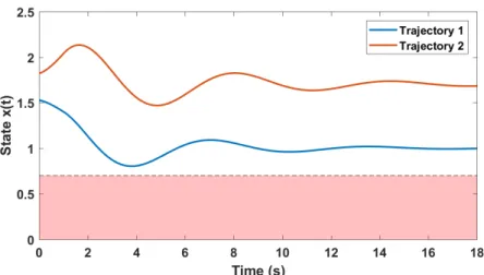
Additionally, one secondary challenge faced during verification is stochasticity and the randomness it introduces into the system dynamics. Stochasticity is present in many physical systems, commonly as process and/or measurement noise in the underlying dynamics. While the system’s trajectories will still vary according to the operating conditions, the stochastic noise terms will also affect the evolution of the states. Due to the randomness introduced by stochasticity, no two simulations or experiments will ever be the same, even if they are performed at the same parameter setting. In fact, when multiple trajectories are performed at the same operating condition, some trajectories may satisfy the designed requirement(s) while others may not, as shown later in Figure 5-1. Ultimately, the fact multiple trajectories at the same operating condition may produce different results means a stochastic system will no longer always satisfy or fail to satisfy the designated requirement at a particular operating condition, but will instead have a probability of satisfying the requirement.
Lastly, the incorporation of prior verification work in the later stages of a multi-stage verification analysis (Figure 1-2(b)) is another secondary challenge. In those problems, it is desirable from a cost perspective to transfer the results from the preceding stages into later stages and speed up the process; the question is how to do this in a correct manner. The differences in the dynamics between lower- and higher-fidelity simulation models will cause inaccuracies in the certification output from the lower-fidelity model. The same type of inaccuracy is experienced between simulation models and experimental results. These inaccuracies are usually slight but their existence does complicate forward transfer of verification output from an earlier
stage of the process into later stages.
1.3 Literature Review
There exists a wide range of verification techniques that have been used to address some form of control system verification or testing. This section will overview these various techniques and discuss their merits or limitations with respect to the verifi-cation challenges identified in Section 1.2.1.
1.3.1 Analytical Verification Methods
Analytical verification encompasses a variety of disparate approaches with either closed-form or numerically-exact solutions for theoretically-proven robustness. For discrete-time dynamical systems, methods originally developed for rapidly-exploring random trees (RRTs) can be used to analyze the closed-loop trajectories from simple linear or linearized nonlinear models. In particular, chance-constrained, closed-loop RRT (CC-CL-RRT) methods [33–35] are able to efficiently propagate the effects of stochastic noise in closed-loop trajectories by placing Gaussian distributions around a nominal trajectory to model the stochasticity in the system’s states. Although this has been demonstrated on relevant aerospace applications [36], the method’s applicability is limited due to it’s reliance upon linear or linearized models. More importantly, there is no readily-apparent extension to incorporate parametric uncer-tainties in non-state variables and the verification analysis would have to be repeated for each realization of the parameterized, linear model.
A second type of approach focuses on finite abstractions of the nonlinear closed-loop dynamics. These approaches either assume the closed-closed-loop dynamics are pre-sented as a finite transition system or approximate the dynamics in such a way. For example, Markov chain analysis methods [37,38] assumes the set of all possible states is a n-dimensional hypercube (or similar shape) and models stochasticity in the dy-namics as transition probabilities between those states. Similar common verification tools such as SpaceEx [39] approximate the state space with a finite lattice and
com-pute the approximate reachability of a hybrid system. Although more recent work [40] has applied parametric transition systems to discretize both the state and parameter spaces in adaptive control problems, the utility of finite transition systems is lim-ited by the discretization of the dynamics. As the complexity of the system grows, the level of discretization required becomes intractable and further exacerbated in high-dimensional systems.
Satisfiability modulo theorem (SMT) solvers [41, 42] verify the 𝛿-satisfiability of logic requirements in overapproximations of the reachable state space. These tech-niques construct proofs to provably guarantee whether a set of requirements will be satisfied given nonlinear differential equations representing the system’s closed-loop dynamics. The approach has also been extended to include stochastic systems [43]. Even though these techniques have been shown to handle polynomial and logrith-mic nonlinear systems with simple discrete mode transitions, they fail to scale well to higher-dimensional and -complexity systems and suffer from the same issues with uncertain parameters as the previous approaches.
The most relevant approach for verification of complex, uncertain nonlinear sys-tems is bounding function-based analysis. As the name suggests, these techniques rely upon analytical functions such as Lyapunov, barrier, or storage functions to bound the reachability of the system’s trajectory. For instance, the Lyapunov func-tion common to MRAC systems defines a convex, quadric hypersurface that bounds the reachable set of states from a given set of initial conditions and parametric un-certainties [1, 44]. More advanced methods like barrier certificates [45–47] and LQR trees [48] can be constructed for a variety of nonlinear systems with stochasticity and complex performance requirements. While these analytical techniques produce extremely powerful certificates that provably verify the set of reachable states, they can be difficult to construct for arbitrary nonlinear systems [49]. The existence and conservativeness of the certificate is tied to the choice in Lyapunov function, but the correct or best function representation may not be known in advance. Likewise, as the complexity or number of states and parameters increases, the minimum complex-ity for an appropriate Lyapunov function also increases and complicates finding a
useful verifying certificate. Recent work [29] has been able apply these techniques to higher-dimensional systems, but does so by introducing additional conservatism. Simulation-Guided Analytical Verification Methods
In order to more easily find and construct analytical certificates, simulation-guided barrier certificates [50–53] and LQR trees [54] were developed to automate the ver-ification process. As the choice of function representation is inherently coupled to the conservativeness of the certificate, but the best choice is generally unknown, it is difficult to compute a maximizing bounding set without prior knowledge or experi-ence. These methods use simulation traces and the gradient of candidate Lyapunov functions to determine suitable Lyapunov functions and calculate their maximizing invariant set, effectively automating the process. These techniques also serve as a bridge between analytical verification methods and statistical ones.
1.3.2 Statistical Verification Methods
On the opposite side of the spectrum, statistical verification methods are brute-force approaches that return statistical certificates or bounds based upon large sets of trajectory data. In comparison to analytical techniques, statistical approaches are much more straightforward, but usually more data intensive. In extreme cases, the system can be treated as a black-box model with zero information on the internal model structure/dynamics.
One popular, recent development is falsification-guided software tools such as Breach [55] or S-TaLiRo [56,57]. These approaches use temporal logic properties and nonlinear optimization to intelligently search for counterexamples to a given perfor-mance requirement and simulation model. Although they have been demonstrated on multiple relevant applications, falsification approaches address a similar, but dif-ferent type of problem. Rather than identify the set of operating conditions for which the system will satisfy the performance criteria, falsification methods utilize optimization techniques to converge towards a single trajectory (counterexample) of
the system that fails to meet the requirement. This underlying optimization pro-cess controls falsification-guided testing and will direct the search towards areas with lower robustness; however, falsification methods may encounter problems similar to those seen in non-convex optimization. Just as optimization may repeatedly fall into the same local optimums, falsification searches may inadvertently return the same counterexample, even if they are initialized at different starting points. While these methods are extremely useful for quickly finding a single counterexample, they are not perfectly suited to problems where multiple counterexamples exist and the goal is to identify the entire set of unsatisfactory operating conditions. For this reason, falsification-guided techniques are of limited use to the particular problem of interest in this thesis.
The most general, widely-used, and versatile approaches are Monte Carlo methods [30,31,58–69]. Part of the reason for their popularity and versatility is their simplicity: they randomly generate a large number of trajectories and reason about the system’s robustness from this finite number of observations. Monte Carlo methods are practical tools for measuring the effects of stochasticity [58–60] and parametric uncertainties [25,26,61,70] in the dynamics and have been used in conjunction with various tools like S-TaLiRo [58,62,63], PRISM [64,65], and other statistical model checking approaches [30,31,66–69]. The main drawback of Monte Carlo methods is that they rely upon the law of large numbers to provide bounds or statistical estimates [59,60], meaning a large amount of data is required. Importance sampling and cross-entropy methods [60,61, 63,67] have been developed to reduce the number of samples required for statistically-relevant results, but are still inherently random and require many samples.
Additional techniques like Dirichlet Sigma point processes [24], set-oriented mod-els [71], and box thresholding [72] all attempt to circumvent the limitations of Monte Carlo approaches with finite, structured groupings. Rather than randomly sample from the set of all operating conditions, these approaches select some subset of condi-tions explicitly chosen for their perceived informativeness about the results over the full set. Design of experiments techniques [73, 74] can also be considered to roughly fall within this category or the intersection between it and Monte Carlo methods.
While these approaches offer an alternative to pure Monte Carlo methods, they can still be viewed as sample inefficient because they rely upon pre-generated grids or lattices covering the set of all possible operating conditions. These structured group-ings will typically require a fine discretization or some equivalent in order to observe the changes in performance satisfaction with adequate resolution and will therefore require a nontrivial number of simulations or experiments.
The closest approach to the work in this thesis are the Gaussian process-based methods for safe learning of regions of satisfactory performance [75,76]. These meth-ods combine Lyapunov analysis from analytical verification techniques with Bayesian optimization to efficiently estimate the region verified by a Lyapunov function-based barrier certificate. While these methods straddle the line between analytical and statistical verification techniques, they ultimately break analytical techniques’ funda-mental assumption of provable guarantees of closed-loop performance with the use of Bayesian predictions. This fact shifts the methods’ implementation closer to statis-tical techniques, but their reliance upon a given Lyapunov function for verification of the system causes them to suffer the same limitations as analytical techniques. In effect, these methods are useful for searching the set of uncertainties to estimate the limits of a barrier certificate, but are not able to provide provable guarantees like the aforementioned analytical methods nor do they posses the same versatility of most statistical methods.
One important observation is that all of the discussed approaches, both analytical and statistical methods, do not present an explicit solution to the challenge of forward transfer of predictions from prior verification stages in a multi-stage process. Although these earlier stages indirectly aid later steps by pruning out unsatisfactory candidate controllers, none of the approaches posses a mechanism for direct incorporation of previous results. In fact, many of these approaches will lose all guarantees once applied to a different model. For instance, barrier certificates are coupled to the model of the system dynamics used to construct the proof and lose any guarantees as soon as the later stage’s dynamics deviate from the original equations. The results from proceeding stages can be used to inform initializations of later steps, but there
is no mechanism to transfer the output. Effectively, the later verification procedure will be performed without any direct knowledge of the earlier predictions or proofs and will have to replicate those results. This presents an obvious inefficiency and can prove extra costly in experiment-based verification if the later experiment-based stage crashes or destroys a prototype at an operating condition that was already identified as dangerous by the preceding stage(s).
1.4 Summary of Contributions
This thesis proposes a unified framework to address all the aforementioned challenges with statistical verification. At a high level, this work combines control system veri-fication with machine learning to produce novel, data-driven procedures for efficient statistical verification in resource-constrained environments. The thesis is structured around three sets of major contributions corresponding to 1) the baseline problem with verification of deterministic systems, 2) verification of stochastic systems, and 3) multi-stage verification (Figure 1-2(b)) with multiple, sequential verification steps. These contributions build upon one another to address the fundamental challenges in Section 1.2.1 that plague efficiency and tractability in statistical verification of complex, nonlinear control systems.
The first major set of contributions concentrates on verification of determinis-tic systems where each reinitialization of the trajectory will produce the same exact result. This work shows deterministic verification is ultimately a binary classifica-tion problem - a trajectory will either satisfy a performance requirement or it will not - and introduces new machine learning algorithms aimed at that problem. The contributions for deterministic verification are as follows:
∙ The development of a new machine learning framework for statistical verification called data-driven verification certificates. Unlike barrier certificate methods, this framework directly translates raw trajectory data into a predictive cer-tificate without intermediate analytical, proof-based steps. These data-driven
to apply to a significantly wider class of systems. Chapters 3 and 4 introduce two parallel modeling techniques each tailored to exploit one of the two most common sources of feedback on a trajectory’s performance.
∙ The introduction of validation techniques for online quantification of prediction accuracy. Section 3.3.1 extends traditional machine learning methods for model validation to data-driven verification certificates and analyzes their effectiveness in statistical verification. Most importantly, Section 4.2.2 designs a completely new approach for online computation of prediction confidence without reliance upon external validation datasets or retraining of the prediction model. This latter validation technique minimizes the amount of additional computational overhead and guarantees the predictive certificate will explicitly answer both relevant questions for each query:
– Is the trajectory going to satisfy the requirements? – How confident is the model in that prediction?
The second question is almost as important as the prediction itself, but is fre-quently not addressed in statistical verification and relevant machine learning techniques.
∙ The development of closed-loop verification algorithms to maximize the accu-racy of prediction certificates while limited to fixed sample budget. A major part of this contribution is the introduction of new entropy-based selection met-rics (Section 4.3) to evaluate the informativeness of prospective trajectories and select future training samples to produce the largest expected improvement in prediction confidence. Several examples demonstrate closed-loop tion’s improvement in prediction accuracy over comparable analytical verifica-tion techniques, open-loop (non-iterative) verificaverifica-tion approaches, and compet-ing iterative procedures adapted from existcompet-ing machine learncompet-ing methods. The second set of contributions extends data-driven verification to stochastic
sys-certificates will no longer apply without heavy modification. This set of contributions reproduces the same high-level concepts behind data-driven certificates and closed-loop verification for the separate and distinct stochastic problem. These contributions include:
∙ The development of data-driven verification frameworks to model the probabil-ity of satisfaction or failure in stochastic systems. Specifically, Chapters 5 and 6 introduce different approaches to model the various distributions of performance feedback evaluations possible with stochastic dynamics. These techniques all predict the likelihood of an unsatisfactory trajectory given a small set of individ-ual trajectories (Chapter 5) or limited groups of repeated trajectories (Chapter 6).
∙ The redevelopment of closed-loop verification algorithms to address the changes with stochastic systems. Sections 5.2 and 5.4 introduce new selection criteria to rank prospective trajectories based upon their expected reduction in prediction error. Several examples in Sections 5.6 and 6.3 again demonstrate the improve-ment in prediction accuracy over open-loop verification approaches afforded by closed-loop verification and the novel selection metrics’ further improvement over relevant procedures adapted from existing machine learning methods. The last major set of contributions in Chapter 7 builds upon the preceding chap-ters to address implementation issues in multi-stage verification. These contributions mainly focus on the value of prior verification work during later stages of the pro-cess and its use to further maximize accuracy in the presence of restrictive testing constraints. The contributions are:
∙ The demonstration of a principled approach for forward transfer of earlier ver-ification analysis of the same control policy on a verver-ification model from an earlier stage. In particular, Section 7.1 details the use of nonzero-mean pri-ors taken from the output of earlier prediction models to explicitly incorporate their effects into later stages. Simultaneously, this approach avoids naïve
as-sumptions about the accuracy of earlier, lower-fidelity models and allows for posterior prediction models to vary drastically from their priors.
∙ The introduction and formalization of a variant of multi-stage verification called failure-constrained statistical verification (Section 7.2). This subproblem con-siders the challenge of statistical verification in experimental domains where unsatisfactory trajectories lead to unacceptable costs. Failure-constrained sta-tistical verification places limits on the maximum allowable number of failures during testing at the experimental stage.
∙ The development of new closed-loop verification algorithms for failure-constrained statistical verification. Section 7.3 introduces two novel algorithms, one adap-tive and one static, to simultaneously minimize the number of failures while maximizing informativeness of the prediction model. Section 7.3 also introduces a new selection criteria specifically tailored to maximize the informativeness of each experiment while limiting the likelihood of failure. Results in Section 7.4 demonstrate the limitations and unacceptable costs of existing procedures when applied to failure-constrained statistical verification and the improvement offered by the new algorithms.
Chapter 2
Background
This chapter introduces and details a number of tools used throughout the thesis. These sections are intended to provide basic background and motivation for the tools as well as present implementation details. Each subsequent chapter will discuss its particular application of these tools and any relevant extensions.
2.1 Support Vector Machines
Support vector machines (SVMs) are one of, if not the, most common tools for binary classification [77–82]. In binary classification problems, the SVM will classify all elements of the feature set Θ ⊂ R𝑝 as either an exclusive element of set Θ
− or its
complement Θ+, where Θ = Θ−∪ Θ+ and Θ−∩ Θ+= ∅. This work assumes there are
only two classes (Θ−, Θ+), although other work has considered SVMs for multi-class
classification [81, 83, 84]. Additionally, set Θ, the set of all feasible features, may be either discrete/countable or uncountable. As will be discussed later in the thesis, this work assumes the feasible set Θ is an uncountable set, but will accurately approximate it with a finely-discretized countable set.
In short, a support vector machine is a supervised learning technique that con-structs an optimum maximum-margin classifier with respect to a set of training data. This training dataset consists of 𝑁 input vectors {𝜃1, 𝜃2, . . . , 𝜃𝑁}with corresponding
con-structed classifier will then predict the label for any arbitrary element of Θ, vector 𝜃 ∈ Θ.
2.1.1 Linear Classifiers
In the simplest form of the problem, it is assumed label 𝑦𝑖 is the output of a linear
model
𝐻R(𝜃) = w𝑇𝜃 + 𝑏, (2.1)
with decision function
𝐻(𝜃) =sign(w𝑇𝜃 + 𝑏) (2.2)
such that 𝑦𝑖 = 𝐻(𝜃𝑖). Elements with w𝑇𝜃 + 𝑏 > 0 are said to belong to set Θ+,
while those with w𝑇𝜃 + 𝑏 < 0 belong to set Θ
−. A linear optimization program can
then be used to compute optimal w and 𝑏 with respect to the training dataset. These terms define a hyperplane in the R𝑝 space that is used to separate 𝜃 datapoints. In
this simplest form, the data is assumed to be linearly separable, meaning there exists two parallel hyperplanes that separate all points with 𝑦(𝜃) = +1 from those with 𝑦(𝜃) = −1. The optimal w and 𝑏 then correspond to the unique maximum-margin hyperplane, which minimizes the distance between the decision boundary given by the hyperplane and any of the training samples [81]. As mentioned earlier, these optimal terms can be computed via the following primal linear optimization problem:
minimize w,𝑏 1 2||w|| 2 such that 𝑦𝑖(w𝑇𝜃𝑖+ 𝑏) ≥ 1 𝑖 = 1, . . . , 𝑁. (2.3)
2.1.2 Nonlinear Classifiers
In practice, the linear model and classifier are not adequate for all types of problems and applications, particularly the ones considered in this thesis. The nonlinearities in dynamical systems often result in nonconvex regions in R𝑝 which simply cannot
classifi-training dataset.
In place of the linear model from (2.1), nonlinear classifiers can be constructed from nonlinear basis functions that are functions of the input vector 𝜃. This new representation is given by
𝐻R(𝜃) = w𝑇𝜑(𝜃) + 𝑏, (2.4)
where 𝜑(𝜃) ∈ R𝑞 is a vector of basis functions and typically 𝑞 > 𝑝. The decision
function 𝐻(𝜃) and the resulting classification rule for elements of Θ− and Θ+ are
mostly unchanged from (2.2), with basis vector 𝜑(𝜃) replacing 𝜃. The new primal optimization program is also similar to (2.3):
minimize w,𝑏 1 2||w|| 2 such that 𝑦𝑖(w𝑇𝜑(𝜃𝑖) + 𝑏) ≥ 1 𝑖 = 1, . . . , 𝑁. (2.5)
In addition to nonlinear models, the baseline SVM classifier can be modified to accommodate datasets which are not linearly separable, as exact separation of the training data by hyperplanes is not possible in many applications [81]. Instead, a soft-margin nonlinear classifier will allow datapoints to fall on the “incorrect” side of the decision boundary, thus enabling a solution where the previous hard-margin SVM would fail. To accommodate possible inseparability in the dataset, a non-negative slack variable 𝜉𝑖 is introduced for each of the 𝑁 training points to relax
the constraints from (2.5). While these slack variables allow for misclassifications, the objective function is also modified with a hinge-loss function in order to penalize these misclassifications and minimize their presence in the optimal solution. The resulting soft-margin primal problem is given by the following quadratic program:
minimize w,𝑏 1 2||w|| 2 + 𝐶 𝑁 ∑︁ 𝑖=1 𝜉𝑖 such that 𝑦𝑖(w𝑇𝜑(𝜃𝑖) + 𝑏) ≥ 1 − 𝜉𝑖 𝑖 = 1, . . . , 𝑁 𝜉𝑖 ≥ 0 𝑖 = 1, . . . , 𝑁 (2.6)
and with a sufficiently-high penalty on non-zero 𝜖𝑖, the soft-margin classifier begins to
operate similar to a hard-margin SVM. Thus, the soft-margin nonlinear SVM is the most general form of classifiers and is capable of handling all the problems previously addressed by the hard-margin, linear and nonlinear SVMs. Due to the fact little-to-nothing is assumed in advance about the performance of the nonlinear systems of interest in this thesis, soft-margin nonlinear SVMs offer the most robust solution with the widest applicability.
Rather than compute the solution using the primal optimization problem in (2.6), it is generally easier to solve the problem in its dual form:
maximize 𝛼 𝑁 ∑︁ 𝑖=1 𝛼𝑖− 1 2 𝑁 ∑︁ 𝑖,𝑗=1 𝛼𝑖 𝛼𝑗 𝑦𝑖 𝑦𝑗𝜑(𝜃𝑖)𝑇𝜑(𝜃𝑗) such that 0 ≤ 𝛼𝑖 ≤ 𝐶 𝑖 = 1, . . . , 𝑁 𝑁 ∑︁ 𝑖=1 𝛼𝑖𝑦𝑖 = 0, (2.7)
with weighting terms now set to w =
𝑁
∑︁
𝑖=1
𝛼𝑖 𝑦𝑖 𝜑(𝜃𝑖). (2.8)
As the dimension 𝑞 of the feature space associated with 𝜑(𝜃) grows, computing the mapping w𝑇𝜑(𝜃) + 𝑏 becomes increasingly computationally demanding. Instead, the
“kernel trick” [79] is used to reduce this cost through a kernel function 𝜅(𝜃, 𝜃′
) : R𝑞× R𝑞→ R, defined such that
𝜅(𝜃, 𝜃′) = 𝜑(𝜃)𝑇𝜑(𝜃). (2.9)
This use of the kernel function enables a solution to the dual problem in (2.7) to be found without having to work in the potentially high-dimensional feature space for 𝜑(𝜃). Various forms of the mapping and kernel functions exist, such as polyno-mial, hyperbolic, and Gaussian radial basis function (RBF) [77,79,81]. In this work,
Gaussian RBFs are used unless otherwise noted. These RBF kernels are given by 𝜅(𝜃𝑖, 𝜃𝑗) =exp(−||𝜃𝑖− 𝜃𝑗||2/𝛾), (2.10)
with 𝛾 > 0. Finally, the decision function for the soft-margin, nonlinear SVM in its dual form is given by
𝐻(𝜃) =sign(︁ 𝑁 ∑︁ 𝑖=1 𝛼𝑖𝑦𝑖𝜅(𝜃, 𝜃𝑖) + 𝑏 )︁ . (2.11)
Note that not all of the 𝑁 training points are considered “active.” Only a subset of the training points are selected as support vectors (𝑁𝑠𝑣 ≤ 𝑁 ); all remaining points can be
considered to have 𝛼𝑖 = 0 and are thus not active. In practice, only the active subset
of 𝑁𝑠𝑣 support vectors are used for predictions, improving computational efficiency.
For the remainder of this thesis, the SVM optimization problem and its decision function will be shown and discussed in the format of the dual representation from (2.7) and (2.11).
2.2 Gaussian Process Regression Models
Gaussian process (GP) regression models, sometimes known as Kriging, are Bayesian nonparametric regression tools for modeling scalar target variables across a continuous input space [85–87]. Gaussian processes have been widely used throughout a variety of relevant applications such as adaptive control [88, 89], reinforcement learning [90, 91], and optimization [92]. In this thesis, GPs are used to model measurements of performance requirement satisfaction by the closed-loop system under consideration. The following material will provide background on the construction of GP regression models and explain certain steps which will be discussed later in the thesis.
While a Gaussian process is formally defined as the joint Gaussian distribution of a finite collection of random variables, it can more easily be thought of as a distribution over possible functions for ℎ(𝜃). Here, ℎ(𝜃) is a real, scalar function with input vector
𝜃 ∈ R𝑝. Additionally, the GP is completely defined by a scalar mean function 𝑚(𝜃)
and covariance function 𝜅(𝜃, 𝜃′
) such that
ℎ(𝜃) = 𝐺𝑃(︀𝑚(𝜃), 𝜅(𝜃, 𝜃′))︀. (2.12)
The overall aim of the GP regression model is to infer the true, but unknown, function ℎ(𝜃) from a limited number of sample locations {𝜃1, 𝜃2, . . . , 𝜃𝑁} and corresponding
observations of ℎ(𝜃), labeled 𝑦(𝜃𝑖). Both the cases where 𝑦(𝜃𝑖)are noisy and noiseless
measurements of ℎ(𝜃𝑖) are considered and will be discussed later. The resulting GP
regression model can then be used to predict function values ℎ(𝜃) at unobserved input vectors 𝜃. Rather than specifying a particular parameterized form of ℎ(𝜃) and attempting to infer the correct coefficients, the GP model treats ℎ(𝜃) as a random function. This allows the GP to be free of any restriction to a parameterized form, assuming one even exists, and improves its applicability.
2.2.1 Training
At its core, Gaussian process regression relies upon Bayesian inference to construct the predictive model. Model training is performed according to Bayes’ rule with a prior probability distribution and likelihood model of the data used to compute a posterior probability distribution. In this problem, the posterior probability distribution defines the distribution of ℎ(𝜃) values conditioned on the evidence provided by the training dataset of 𝑁 sample locations and corresponding observations mentioned earlier. For simplicity, this training set is labeled as ℒ = {𝒟, y} where set 𝒟 = {𝜃1, . . . , 𝜃𝑁}
contains the input locations and vector y = [𝑦(𝜃1), . . . , 𝑦(𝜃𝑁)]𝑇 is the corresponding
observations. The underlying true function values of ℎ(𝜃) at these training locations are labeled as vector h = [ℎ(𝜃1), . . . , ℎ(𝜃𝑁)]𝑇. The posterior distribution of h is
determined from the likelihood model formed by the observations in ℒ and a pre-specified prior probability distribution for h.
The prior probability distribution for h is assumed to be a joint, multivariate Gaussian distribution defined by mean vector m = [𝑚(𝜃 ), . . . , 𝑚(𝜃 )]𝑇 and 𝑁 × 𝑁
covariance matrix K = [𝜅(𝜃𝑖, 𝜃𝑗)]for 𝑖, 𝑗 = 1, . . . , 𝑁,
P(h|𝒟, 𝜓) = 𝒩 (h|m, K). (2.13)
The term 𝜓 refers to the kernel function’s hyperparameters. While there are many different possible kernel functions, this thesis always uses the default squared expo-nential kernel function with automatic relevance determination (SE-ARD) for GPs. The SE-ARD kernel is an RBF kernel much like the kernel in (2.9) for SVMs,
𝜅(𝜃, 𝜃′) = 𝜎𝑓2exp{−0.5(𝜃 − 𝜃′)𝑇Λ−1(𝜃 − 𝜃′)} (2.14)
Λ =diag(𝜎12, 𝜎22, . . . , 𝜎𝑝2),
but with a weighting term 𝜎1, . . . , 𝜎𝑝 for each dimension in 𝜃 ∈ R𝑝. The
ker-nel hyperparameters 𝜓 is the set of these terms along with the signal ratio 𝜎𝑓,
𝜓 = {𝜎𝑓, 𝜎1, . . . , 𝜎𝑝}. In comparison to isotropic squared exponential kernels,
SE-ARD enables the hyperparameters associated with each element of 𝜃 ∈ R𝑝 to vary
independently. Combined with the hyperparameter optimization process in Section 2.2.3, this allows the GP training process to automatically discover elements with low impact on ℎ(𝜃) and deemphasize them with a low 𝜎𝑖 or emphasize those with high
sensitivity with large 𝜎𝑖.
In addition to the choice of kernel function for K and its hyperparameters 𝜓, the prior mean m has a large impact upon the trained GP regression model. In the vast majority of applications, the prior mean m is set to 0 [85]. This ensures an unbiased prior probability distribution and has been shown to produce good results for countless problems [86], assuming 𝑁 ≫ 𝑝. The same zero-mean prior is used throughout the thesis, except for specific applications discussed in Chapter 7.
The likelihood model given the observations can be factorized amongst each of the 𝑁 training points
P(y|h, 𝜗) =
𝑁
∏︁
𝑖=1
where 𝜗 is the set of hyperparameters associated with the likelihood model. The posterior probability distribution for h is computed from Bayes’ rule
P(h|ℒ, 𝜓, 𝜗) ∝ P(y|h, 𝜗) P(h|𝒟, 𝜓). (2.16)
2.2.2 Predictions
The posterior probability distribution from (2.16) is then used predict the distribu-tion of ℎ(𝜃) at unobserved points in the input space condidistribu-tioned on the observed data ℒ. These unobserved query locations, assume 𝑁* in total, are labeled 𝒟* and
h* denotes their values of ℎ(𝜃). According to the GP prior in (2.13), the joint
proba-bility distribution of the training h and the prediction h* is a multivariate Gaussian
distribution P(h, h*|𝒟, 𝒟*, 𝜓) = 𝒩 (︃⎡ ⎣ h h* ⎤ ⎦ ⃒ ⃒ ⃒ ⃒ ⃒ ⎡ ⎣ m m* ⎤ ⎦, ⎡ ⎣ K K* K𝑇* K** ⎤ ⎦ )︃ . (2.17)
Note that the covariance matrix pictured is segmented into three components for easier viewing: the 𝑁 × 𝑁 covariance matrix K from the training data, K** the
𝑁* × 𝑁* covariance matrix of the query locations, and the 𝑁 × 𝑁* cross-covariance
matrix K*between the two sets of 𝜃 locations. From this, the conditional distribution
of h* given h is also a multivariate Gaussian,
P(h*|h, 𝒟, 𝒟*, 𝜓) = 𝒩(︀m* + K𝑇*K −1
(h − m), K**− K𝑇*K −1
K*)︀. (2.18)
Ultimately, the desired posterior predictive distribution of h* is the conditional
dis-tribution (2.18) marginalized over the posterior disdis-tribution (2.16), P(h*|ℒ, 𝒟*, 𝜓, 𝜗) =
∫︁
P(h*|h, 𝒟, 𝒟*, 𝜓) P(h|ℒ, 𝜓, 𝜗) 𝑑h . (2.19)
This posterior predictive probability distribution will change based upon the likeli-hood model of the observations. The two cases to consider are whether the
observa-tions of ℎ(𝜃) are noisy or noise-free. Noise-free Observations
The first case assumes the measurements of ℎ(𝜃) are noise-free, meaning y = h. Since ymeasures h directly, there is no posterior uncertainty about h after the observations. The posterior predictive distribution of h* reduces to
P(h*|ℒ, 𝒟*, 𝜓, 𝜗) = 𝒩(︀m*+ K𝑇*K −1
(h − m), K**− K𝑇*K −1
K*)︀, (2.20)
which is simply the conditional distribution (2.18). Noisy Observations
In the other case, the observations of ℎ(𝜃) are assumed to be corrupted by some noise term that prevents y from measuring h directly. Many possible types of noise exist, the simplest of which is the standard uniform Gaussian noise assumption made by the vast majority of GP literature [85–92]. The following paragraphs will discuss GP predictions using observations corrupted by uniform Gaussian noise. Later chapters will discuss variations on this noise model as they apply to problems of interest.
In the standard problem, the observations y are corrupted by a noise term 𝜖, which is assumed to follow a uniform Gaussian distribution 𝜖 ∼ 𝒩 (0, 𝜖2
𝑛) such that
𝑦(𝜃) = ℎ(𝜃) + 𝜖 and
P(y|h, 𝜖𝑛) = 𝒩 (y|h, 𝜖2𝑛). (2.21)
Due to the fact the noise variance 𝜖𝑛 is 𝜃-invariant and constant across the space,
uniform Gaussian noise is also referred to as homoscedastic Gaussian noise. When noise variance 𝜖𝑛 is known in advance, likelihood model hyperparameters 𝜗 = 𝜖𝑛 and
the likelihood model for the observations can be written as
![Figure 3-6: [Example 3.5.1] Comparison of sample selections for batch sizes of](https://thumb-eu.123doks.com/thumbv2/123doknet/14539521.535260/79.918.163.771.203.425/figure-example-comparison-sample-selections-batch-sizes-.webp)
![Figure 3-13: [Example 3.5.2] Effect of increasing false-positive penalties in the SVM predic- predic-tion model](https://thumb-eu.123doks.com/thumbv2/123doknet/14539521.535260/86.918.270.622.118.391/figure-example-effect-increasing-positive-penalties-predic-predic.webp)
![Figure 3-14: [Example 3.5.3]: Comparison of the misclassification error convergence of open- open-and closed-loop statistical verification techniques](https://thumb-eu.123doks.com/thumbv2/123doknet/14539521.535260/88.918.280.619.126.396/figure-example-comparison-misclassification-convergence-statistical-verification-techniques.webp)
![Figure 4-8: [Example 4.4.1] Final prediction model after 350 samples. The resulting pre- pre-diction boundary separating Θ̂︀](https://thumb-eu.123doks.com/thumbv2/123doknet/14539521.535260/120.918.147.755.582.823/example-prediction-resulting-separating-.webp)
![Figure 4-9: [Example 4.4.1] Misclassification error convergence of Algorithm 6 in comparison to the other approaches over the same 100 random initializations](https://thumb-eu.123doks.com/thumbv2/123doknet/14539521.535260/121.918.151.759.124.381/figure-example-misclassification-convergence-algorithm-comparison-approaches-initializations.webp)
