Application of the homotopy continuation method to low-eccentricity preliminary orbit determination

Application of the Homotopy Continuation Method to

Low-Eccentricity Preliminary Orbit Determination

by

Andrew Markland Stanley Hart

Submitted to the Department of Aeronautics and Astronautics on June, 1991, in partial fulfillment of the

requirements for the degree of

Master of Science in Aeronautics and Astronautics

Abstract

The homotopy continuation method is a method for solving a set of non-linear equa-tions.

This thesis examines the application of the homotopy continuation method to the preliminary orbit determination of satellites with low eccentricity orbits, extending and modifying techniques of R. L. Smith and C. Huang. Further improvements to the method, to allow more general orbit determination, are considered.

In particular this thesis deals with orbit determination using only six range mea-surements from a single ground-based tracking station. Application to the Landsat 6 satellite, which is due to be launched in May 1992, is considered.

Thesis Supervisor: Richard Battin

Title: Professor of Aeronautics and Astronautics

Thesis Supervisor: David W. Carter Ti tIe: Staff Member, Draper Laboratory

Acknowledgments

I would like to thank David Carter of The Charles Stark Draper Laboratory for the invaluable time and assistance he provided over the last eight months.

I would also like to thank the Massachusetts Institute of Technology for the finan-cial aid provided by it during that time.

A final note of thanks goes to Professor Richard Battin for his instruction in courses 16.46 and 16.47, which were both interesting and directly applicable to this work, for providing me with the opportunity to work on this subject and for acting as my thesis supervisor.

Biographical Note

The author graduated with first class honors in June 1989 from the University of Southampton, England, with a Bachelor of Engineering degree in Aeronautical and Astronautical Engineering.

While at The Massachusetts Institute of Technology the author spent six months as a research assistant doing experimental work in The Wright Brothers Wind Tunnel.

Contents

1 Introduction

1.1 Motivation.

1.2 Previous Work Concerning Preliminary Orbit Determination

9

9

11 1.3 Previous Work Concerning The Homotopy Continuation Method. 11

1.4

Outline of Thesis 12

2

The Method

2.1

Setting Up the Problem 2.2 Mechanics of the Method . .

2.3

Direct Newton- Raphson

2.4

Screening

...

3

Curve Following Algorithm

3.1

Starter . . . .

3.2

Step Size Selection

3.3

Predictor ..

3.4

Corrector

3.5

Monitor

..

3.6

Arc Length Correction

3.7

Solution State Collection

3.8

Critical State Collection

3.9

Termination of the Algorithm

3.9.1

Normal Termination

.

.

...

13

13

15

21

22

25

26

27

28

29

32

33

37

41

45 45

3.9.2

3.9.3

Optional Termination. . Abnormal Termination . 46 46

4 Details of the Newton-Raphson Corrector Scheme

5

Problems With the Algorithm

5.1 Algori thm Failure . . . 5.2 Inaccurate Results 48 58 59 63

6

Removing The Brouwer-Lydanne Singularity at Critical Inclination

66

7

Application to the Landsat Satellite

7.1 Landsat 4 Test Cases .

7.2 General Comments

8

Use of the Software

9

Conclusions

10

Recommendations for Future Work

10.1 The Extended Six-Level Scheme .. 10.2 Allowing for Hyperbolic States. 10.3 Sensitivity Study . . . .

lOA Atmospheric Drag Modeling

10.5 Improved Gravitational Field Modeling 10.6 Application to Non-Terrestrial Satellites

APPENDIX A

APPENDIX B

72

74

82

84

87

89

89

90

91

91

93

93

97

99

List of Figures

2-1 Schematic Diagram of a Simple Solution Curve 16

2-2 Schematic Diagram Showing the Possible Effects of Varying the A

Pri-ori Estimate on the Shape of the Solution Curve 17

2-3 Schematic Plot Showing a Case Where the A Priori Estimate and the Solution Which We Seek Lie on Different Loops . . . 19 2-4 Schematic Diagram Illustrating the Corrector Scheme Employed 20 2-5 Schematic Diagram of a Case Where the Simple Newton-Raphson

Method May Converge to the Wrong Solution . . . .. 23 2-6 Schematic Diagram of a Case Where the Simple Newton-Raphson

Method May Diverge 24

3-1 Schematic Diagram Illustrating How Correcting With Constant ..\Could

Cause Problems 30

3-2 Schematic Example of the Solution Curve Doubling Back 34 3-3 Schematic Example of the Solution Curve Skipping a Portion of the

Solution Curve Where it Pinches In 35

3-4 Schematic Diagram to Show the Effect of Limiting ..\ Step Between

Consecutive Points on the Solution Curve 36

3-5 Schematic Diagram Showing Potential Problem With Solution State

Collector 39

3-6 Schematic Diagram Showing Another Potential Problem With Solution

3-7 Schematic Diagrams Representing the Different Discard and Reset

Sce-narIOS 44

4-1 Simple 2-D Example Showing Why a Convergence Criterion on the

Size of the Correction Vector can be Poor 56

5-1 Plots Showing the Changing Shape of a Solution Curve as the A Priori

Epoch Estimate is Varied in a Real Case . . . .. 61

6-1 Plots of Exact and Replacement Factor vs Inclination 68 6-2 Plot of Replacement Function Divided by Exact Function vs

Inclina-tion 69

6-3 Plot of Inclination vs A Using the Exact Factor in a Real Case 70 6-4 Plot of Inclination VB A Using the Replacement Factor in a Real Case 71

10-1 A Plot Showing That Eccentricity on the Solution Curve Can be Large Even if the A Priori Estimate and the Real Solution Have Very Low Eccentricities . . . .. 92

Chapter

1

Introduction

The purpose of any satellite orbit determination method is to use tracking data to determine the orbit of a satellite at some epoch time so that predictions regarding the future path of that satellite can be made. This research addresses the use of the homotopy continuation method with only six range measurements from a single Earth based tracking station for orbit determination. A range measurement is simply a measurement of the distance between the tracking station and the satellite.

1.1

Motivation

Up until recently the Landsat program was owned and operated by the United States government (NASA). The tracking data available to the program consisted of range, range-rate and angle data from a number of different Earth tracking stations, as well as data from the Tracking and Data Relay Satellite System (TDRSS).

In 1984, the Landsat Remote Sensing Commercialization Act was passed by Congress. This act allowed a contract for the operation and expansion of the Landsat system to be awarded to a private firm through competitive bidding. The contract was awarded in September 1985 to the Earth Observation Satellite Company (EOSAT) which is based in Lanham, Maryland.

EOSAT is a partnership formed in 1984 by General Motors' Hughes Aircraft Com-pany, the General Electric Astro-Space Division, and Computer Sciences Corporation.

EOSAT is responsible for the development of the new Landsat and for worldwide marketing of Landsat data.

It

has initiated the development of the next generation Landsat satellite, Landsat 6.

EOSAT currently receives ephemeris and payload data from the .Goddard Space Flight Center( GSFC) in Greenbelt, Maryland, and through the Tracking and Data Relay Satellite System. Tracking data consisting of range, range-rate, and angle data is processed at NASA GSFC. This means that EOSAT does not have control over what data they receive. Also, they have to pay for that data. For these reasons, EOSAT is planning to replace the NASA and other u.S. Government facilities with its own facilities for Landsat 6. This will include a tracking and data reception station in Norman, Oklahoma.

Range-rate is measured by observing the Doppler frequency shift between the satellite transponder and the tracking station receiver. The planned Landsat 6 transponder will be operating at frequencies which experience a maximum of about only 2Hz Doppler shift horizon-to-horizon [10]. This means that range-rate measure-ments would have poor resolution. EOSAT plans to have some angle measurement equipment in the tracking station, but angle measurements are sensitive to atmo-spheric refraction, especially when the satellite is low over the horizon, and so may not be accurate enough to use for preliminary orbit determination. A preliminary or-bit determination method that requires only range measurements seems desirable. An in depth discussion of the history and functions of Landsat and EOSAT is contained in reference [11].

Out of the desire for a preliminary orbit determination method which requires only range measurements from a single Earth-based tracking station comes the motivation for the adaptation of the homotopy continuation method presented in this thesis.

1.2

Previous Work .Concerning Preliminary

Or-bit Determination

A variety of techniques using varying combinations of range, range-rate and angle data have been researched in the past. A number of the classical orbit determi-nation methods are presented in reference [9]. Chapter 9 of reference [8] presents algorithms using range and angle data. In reference [13] a preliminary orbit deter-mination method using satellite-to-satellite range and range-rate data is presented. Reference

[14]

presents a method requiring range-only data from a single station but the method only applies to circular orbit determination. Another range-only method is presented in reference [15], but the method is a least squares method and so has a limited radius of converegence, and it also uses satellite-to-satellite tracking.

1.3

Previous

Work Concerning

The Homotopy

Continuation Method

Many of the ideas for this research were derived from a National Aeronautics and Space Administration technical memorandum by R. L. Smith and C. Huang [1]. That memorandum addr~ssed a similar early orbit determination problem, based on the use of range and range-rate observational data as obtained from the Tracking and Data Relay Satellite System (TDRSS). In this work, only range data obtained from a single Earth-bound tracking station is considered.

A more condensed and easier to read version of the technical memorandum men-tioned above can be found in an American Institute of Aeronautics and Astronautics paper by the same authors

[2].

A theoretical basis for the homotopy continuation method is presented in refer-ence

[3].

Examples of the homotopy continuation method applied to several engineer-ing problems, not including orbit determination, are provided in reference

[6].

1.4

Outline of Thesis

This chapter presents some of the practical background that led to this particular piece of research and provides information about related research. Chapter 2presents a description of the homotopy continuation method as applied to preliminary orbit determination. Chapter 3 describes each of the steps in the algorithm designed to solve the early orbit determination problem. Chapter 4 presents a detailed discussion of the Newton-Raphson corrector step which is the major computational step in the algorithm. Chapter 5 discusses the problems associated with this method of preliminary orbit determination. Chapter 6 contains a discussion of the trick used to overcome the singularity at inclination ~ 63.50 _{in the Brouwer-Lyddane orbit}

propagator. Chapter 7 contains a sample of the results produced by running the program on some real Landsat 4 data. Chapter 8presents a good strategy for using the software developed during this research. Chapter 9 provides a list of the conclusions drawn from this research. In Chapter 10, recommendations for how this work could be extended and improved are suggested. Appendix A contains a brief description of the Gaussian quadrature technique for evaluating integrals. Appendix B contains a user's guide, provides information about the computer subroutines used in' this research, and also contains complete source code of the main program and all of the su b- programs.

Chapter

2

The Method

2.1

Setting Up the Problem

The problem is to carry out orbit determination of artificial satellite using only six range (distance between the tracker and the satellite) measurements from a single Earth based tracker. The method that is employed is the homotopy continuation method.

A clear and simple statement of the objective of this method is as follows: Given the following data:

• the Earth-fixed coordinates of a single tracking station

• the right ascension of Greenwich at some epoch time

• six fixed times relative to the epoch time

• six range observations at those six fixed times relative to epoch

• an a priori estimate to the satellite state at epoch

• an orbit state propagation model, that is, some orbital dynamics model such as two-body mechanics

Calculate the exact satellite state at epoch. In this thesis a satellite state consists of a set of six orbital elements.

Let a general epoch orbit state be represented by x, a general set of six ranges at the six observation times be represented by y and the function that maps the epoch state to the ranges be represented by f. This function includes an orbit prop-agator which propagates the epoch state to a current state at each of the six chosen times. Then those current states are converted to inertial Cartesian coordinates. The tracking station's position in inertial Cartesian coordinates, at each of the times, is also computed. Finally, the root sum of the squares is used to compute the ranges from the satellite and station positions at each of the six times. Note that f depends implicitly on the six times chosen and on the propagation model.

The a priori estimate of the epoch state is denoted by Xed, the set of ranges

calculated by evaluating

f(

Xed) is denoted by Yed and the observed set of ranges is

denoted by Ye:s:. Then, we can say that by definition:

(2.1)

and the problem may be restated as a search for the exact epoch state Xe:s:that solves

the equation :

(2.2)

Now consider the general set of ranges y given by :

(2.3)

where A is the homotopy parameter.

Consider also, the locus of solutions

(A,X)

to the equation:

(2.4)

Clearly, for A = 0,Xed is a solution and for A

=

1,Xe:z:is a solution. Note however

that for any given value of A the number of solutions to equation 2.4 may be zero, one, or more.

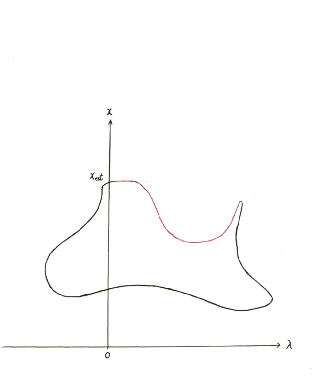
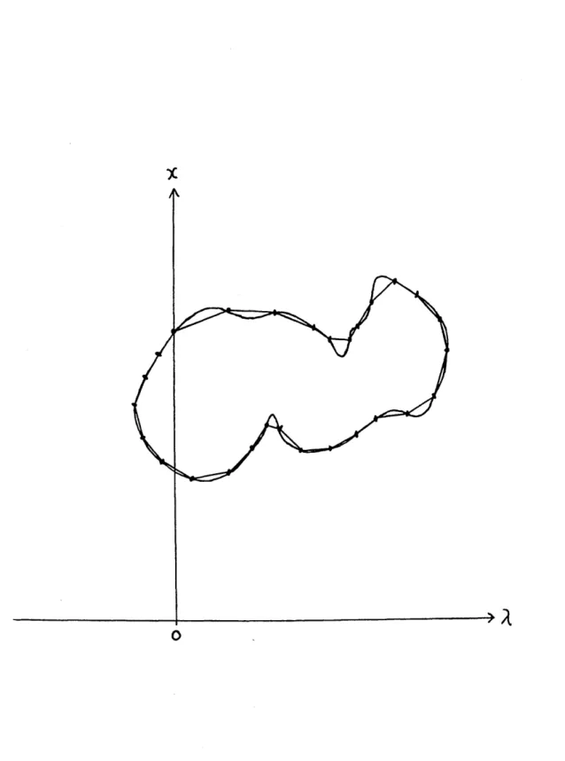
to equation 2.4 in the seven dimensional A~X space, is a set of one or more disjoint,

smooth, closed loops. A very simple example of a possible solution curve is shown in figure 2-1.

From the figure it is evident that in this simple case there is one solution at A

=

1, one solution at A

=

0, two solutions for all A in the range 0

<

A

<

1, and no solutions with A

<

0 or with 1

<

A.

It

is constructive at this point to consider the effect on the shape of the solu~ tion curve( s), of changing the a priori estimated epoch state, Xed' while keeping the

remainder of the problem parameters constant.

Logically, a different a priori estimate should have no effect whatsoever on the actual solution states, i. e. , the

A

=

1solutions. This is borne out by the fact that the set of ranges y given by equation 2.3 for A

=

1 is always Yez and so is independent of Xe6t. For all other values of

A

we would expect solutions to change as

Xed is changed, and so the overall solution curve should change shape. Furthermore,

we should expect that if the a priori estimate is varied smoothly, so too would the shape of the solution curve. Figure 2-2 shows an example of this taking place.

This figure serves to illustrate an additional point: as the a priori estimate varies, the solution curve can smoothly separate into two loops and in fact, for some special a priori estimate, the solution curve will be at a transition point between being one loop with two lobes and being two. separate loops. The significance of this type of transition point will be discussed later on in this thesis after the mechanics of the method have been addressed, something which will be dealt with in the very next section.

2.2

Mechanics of the Method

Theoretically, the method simply entails following the solution curve in the seven dimensional

(A,

x) space around from the a priori state, which is a point at ..\

=

0 on the curve, through all the ..\

=

1points( candidate solutions), recording them as we pass, back to initial start point at A

= o.

It

may be necessary to screen the solutions

x

o

1

x

----4---+--~i\

o t

o

X

o

t

CD

I 1

Figure 2-2: Schematic Diagram Showing the Possible Effects of Varying the A Priori Estimate on the Shape of the Solution Curve

in some way in order to pick out the solution which we seek. That is, the solution which agrees with existing a priori knowledge and which is sufficiently accurate to be useful for making good predictions about the satellite state at future times.

At this time, it should be pointed out that in a case where more than one disjoint loop exists there is no guara~tee that your a priori estimate will lie on the same loop as the solution which you seek [see figure 2-3J. However, it was found that the more accurate the a priori guess, the more likely it will be that that guess and the solution which you seek will lie on the same loop. What needs to be done if this ideal situation does not exist will be dealt with later on in this thesis. For now, it is constructive to assume that a good a priori estimate exists and so the a priori estimate and the solution which you seek do lie on the same loop. For the Landsat 6 case this a reasonable assumption because it will be launched southwards from the Western Test Range (WTR) in California and so its ascending node will have longitude very close to 180°+ the right ascension of WTR (which depends on the time of launch). Also, its inclination will be accurately known (~

98°).

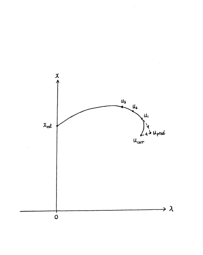
The curve following scheme is a simple predictor-corrector scheme. It consists of using three points on the loop that have already been calculated, to predict what another point further along the loop will be, and then to correct that prediction using a Newton-Raphson iterative scheme. Figure 2-4 illustrates this scheme.

The prediction is made according to quadratic Lagrange extrapolation of the so-lution curve by some previously determined curve length. There is a problem at the start because we only have one known point initially, that is, our a priori estimate. Thus, a special starter scheme is needed for calculating the second point along the loop. Once the second point has been found, those two points can be used to make a prediction based on linear extrapolation, which can then be corrected to give a third point. After each point is corrected, there are a number of procedures that need to be carried out before the next prediction step. A summary of the overall algorithm is shown below :

starter Implement starter scheme to get the second point along the loop and calcu-late the arc length between the two points on the loop.

o

1

Figure 2-3: Schematic Plot Showing a Case Where the A Priori Estimate and the Solution Which We Seek Lie on Different Loops

x

o

step size selector Calculate the step-size (in terms of arc length) that should be taken between the last point and the next point along the curve.

predictor Predict the next point using an extrapolation of the existing points and the step-size calculated.

corrector Correct that prediction using a Newton-Raphson iterative scheme with the prediction as an initial guess.

monitor Ensure that the corrector scheme converged and that the tangent vector at each of the last two corrected points do not differ by much. If either of these is not true, then return to the previous predictor step with a step-size that is halved.

arclength corrector Correct the arc length between the last two corrected points because during the transition from predicted point to corrected point the arc length may have changed from the initial step-size.

solution state collector Check for and store any crossings of the ,\

=

1hyperplane (candidate solutions)

critical point collector Check for and store any points that are extrema in,\. Such points are called critical points.

terminator Check for a return to the initial start point to see if the loop has been completed. If it has, terminate the algorithm. If not, return to step 2.

A more in depth description of each of these algorithm steps is the subject of the next chapter.

2.3

Direct Newton-Raphson

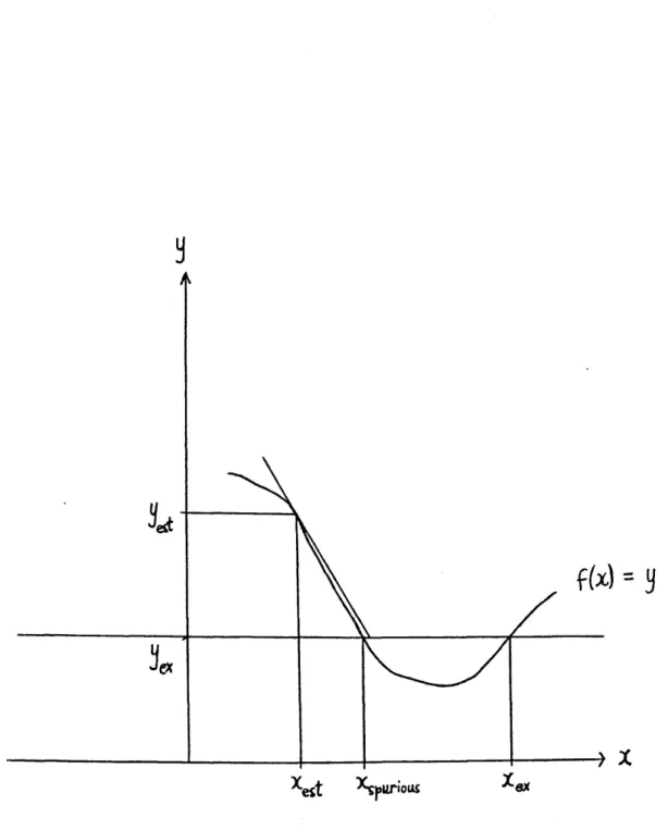
The more simplistic approach of applying the Newton-Raphson method directly to the non-linear equations is not satisfactory. One reason is that the Newton-Raphson

method has a very limited radius of convergence. That is, even a good a priori esti-mate can result in the Newton-Raphson scheme diverging. The second reason is that the problem can have several solutions and so even if the Newton-Raphson scheme converges it may converge to a spurious solution. That is why we need a method that collects

all

of the possible solutions and then screens out the solution which we seek. Figure 2-5 illustrates a case where the simple Newton-Raphson scheme converges to the wrong solution. Figure 2-6 illustrates a case where the simple Newton-Raphson scheme diverges.

An interesting study of the application of the Newton-Raphson method applied directly to the Landsat

6

problem is presented in reference

[16].

2.4

Screening

The screening method would depend on how much a priori information was available about the satellite. For example, some of the solutions may be ruled out by the fact that the amount of energy associated with that state may be greater than the maximum amount of energy that the launch vehicle was capable of imparting to the satellite. Possibly some of the solutions may have inclinations or ascending nodes outside of the limits within which the real inclination or ascending node is known to lie from a priori knowledge. Other solutions may be ruled out by the rough angle measurements made at the tracking station. However, even if there was absolutely no prior knowledge about the vehicle, we could use redundant observations to screen out the solution which we seek. In the case of Landsat orbit determination we will have good a priori knowledge and so we would not have to resort to using redundant observations as a screening method.

f(x)

=

Y

Xest

Figure 2-5: Schematic Diagram of a Case Where the Simple Newton-Raphson Method May Converge to the Wrong Solution

x.

Xest

F~gure 2-6: Schematic Diagram of a Case Where the Simple Newton-Raphson Method May Diverge

Chapter

3

Curve Following Algorithm

This chapter describes each of the steps in the algorithm in some detail, noting in particular any differences from the Smith paper

[1],

and giving reasons for those differences. The first difference to note is that Smith defined his orbit state in terms of position and velocity coordinates, while for this thesis, orbit states are defined in terms of orbital elements.

The algorithm is divided into nine steps, a starter step and then eight other steps which are repeated cyclically until the loop is completed. A good way to regard the starter is to consider it as the first cycle of eight steps; some of the steps in this cycle are left out because they are unnecessary and others are done differently because there is very limited information at the start.

A little notation is constructive at this point. A general point in the seven dimen-sional curve space is denoted by u where u

=

(;\,x). Distance along the curve from the start point is denoted by s and step size is denoted by

8s.

The last corrected point on the solution curve is denoted by Ut, the one before last corrected point on

the solution curve is denoted by U2 and its predecessor is denoted by U3- A predicted

curve point is denoted by Upred- The a priori point which is the first point on our

I . .. () ( (1) (2) (3) (4) (5) (6))

3.1

Starter

The technique used in the starter is as follows :

• Arbitrarily select a step size 5s

=

5sarb •

• Correct that prediction using a Newton-Raphson iterative corrector. The cor-rector scheme will be discussed in in the Corrector section of this chapter .

• If the iterative scheme fails, then change the prediction to

and try the corrector on that. If that fails, change prediction to

and try the corrector on that. If after going through this process of adding 5s to each of the components of Ued in turn, the iterative scheme has not converged

in any case, then let 5s = 5sarb

/2

and repeat the process. Keep halving 5s

until the iteration scheme converges and you have your second point on the solution curve.

Three important points to note here:

1. Assuming that the data is correct, the starter cannot fail although it may require

5s to be quite small.

2.

It

is better to make 5sarb small in the first place. This may save time in that the

algorithm will not have to go through the whole cycle too many times before a successful convergence takes place. Also , it ensures that the first step is a small one and so the arc length between the first two points can be accurately approximated by assuming the curve is straight between those two points.

. 3.

68

should really be scaled according to which component of

Ue.t

it is being added to. For example, adding 0.1 to an eccentricity of 0.001 changes the orbit a great deal more than adding 0.1 km to a semi-major axis of 8000 km.

The starter has parallels to the first five of the eight steps in the main cycle. It has step-size selection (arbitrary), it has a predictor (adding

68

to components of

ue.t),

it has the Newton-Raphson iterative corrector, it has a monitor

(if

corrector does not converge try adding

68

to a different component of Uut) and it has an arc

length corrector which calculates the arc length instead of simply using the

68

that led to convergence.

The three of the eight steps in the main cycle that have no parallels in the starter are omitted for good reasons. The critical state collector needs three corrected points to make sense, and so cannot be included. It is justifiably assumed that we could not have followed the entire loop around in just one small step, and so a check for termination is not necessary at this stage. Since the algorithm has been set up such that the first step is a small one, the curve cannot cross the

A

=

1hyperplane after that first step. Thus, a solution state collector is not necessary at this stage.

3.2

Step Size Selection

The selection of the step size for the next step along the loop depends on the last step size and on the number of iterations the corrector required for convergence at the last step. The maximum number of iterations allowed is set to be 10. That is,

if

the corrector performs 10 iterations and has not converged to the limit required, then a non-convergence is recorded even though the corrector may have been converging slowly. The step size selector says that if the number of iterations was 9 or 10, then the next step size is equal to the last step size. If the number of iterations was less than 9, then the step size is chosen to be a factor of 1.4 times the last step size. My experience with the selection of step size indicates that it makes little difference what number of iterations is used as the limit between increasing step size and leaving it as is. However, Smith [1] suggests that a more complicated step size selection scheme

can lead to a more time efficient algorithm.

The effect of the step size selector is that the algorithm automatically uses rela-tively small steps in areas where the solution curve has a small radius of curvature, and ':!ses relatively large steps in areas where the radius of curvature is large.

3.3

Predictor

The predictor of the next point on the loop uses Lagrange extrapolation based on the last three corrected points and the chosen step size to predict the next point, except when only two corrected points are known, i. e. , immediately after the starter. In that case, the extrapolation is based on only those two points. Note that the extrapolation could be based on any number of previous corrected points but the greater the number of points used, the more computation per step required, and there is no reason to believe the predictions will be better. Smith

[1]

notes that he found

3

or 4 to be an optimum number of back points to use. I found 2 or 3 to be optimum depending on the particular case.

The formulae used for the prediction are shown below, but first a little notation. To be consistent with notation already used, let 81 be the arc length up to the last

corrected point, 82 be the arc length up to the one before last corrected point, etc.

Let 8pred be the arc length at the predicted point, 8pred

=

81

+

08. Finally, let the

number of back points being used be denoted by n. Set

n

Upred

=

L

Li Ui

i=1

where the Lagrange coefficients

(L

i) are calculated according to : j=l j #i L_i

=

--n---II

(Si -

Sj) j=l j#i

3.4

Corrector

i = 1, ... ,n

(3.2)

The algorithm arrives at the corrector with a guess at a point on the solution loop,

Upred. The guess is corrected to a true point on the solution curve using an iterative

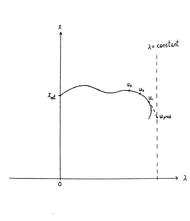
Newton-Raphson scheme. We can take one of two approaches to the problem of correcting this guess. We can insist on keeping A constant and correcting the X part

of Upred. ~his approach has the potential for leading to problems. For example, if

the curve is nearly parallel to a A hyperplane, as it will be near critical points, then convergence may be slow, leading to prohibitively small steps in that area. This point is illustrated by figure 3-1.

The other approach, which is the one used in this thesis, is to allow A to be a variable in the corrector scheme and to introduce the constraint that the correction at each iteration must be perpendicular to the tangent vector of the curve. For maximum accuracy the tangent vector should be calculated at the latest iterated value for the predicted point.

Each iteration involves solving a system of seven equations in the seven vari-ables, A,

x.

One equation is derived from the correction vector constraint. The other six equations are derived from making a linear Taylor Series approximation of equation 2.4 which is reproduced here as equation 3.3

A =

cons to.nt

I

I I

I

I

I

~ I

\

{ u

red.

I

P

o

Figure 3-1: Schematic Diagram Illustrating How Correcting With Constant A Could

The constraint equation is given by :

du

-

.5u

=

0

ds (3.4)

The evaluation of ~~ is discussed in detail in the next chapter.

Let a point on the solution curve be denoted by U.ol where U.ol

=

('\.01,

X.ol). This

point will satisfy equation 3.3 giving:

Rewri ting U.ol as :

U.ol

=

Upred

+

5u

=

('\pred

+

5'\,

Xpred

+

Sx)

and substituting equation 3.6 into equation 3.5 gives:

(3.5)

(3.6)

Now expanding the left hand side of equation 3.7 in a Taylor series and discarding the non-linear terms gives:

(3.8)

Equating the right hand sides of equation 3.7 and equation 3.8 gives :

Rearranging equation 3.9 gives us the six equations to go along with the constraint equation in making up the complete system of seven.

where

f( x)

IX=Xpnd is the set of six ranges calculated by propagating the predicted

state to the six chosen times, and

f'(x)

IX=Xpnd is the six-by-six matrix of partial

derivatives of those six ranges with respect to the six epoch orbital elements.

After the seven-by-seven system has been solved, the resulting 5u is added to the predicted state to give the new predicted state to be used in the next iteration. This process is repeated until the convergence criterion has been met or until the maximum ten iterations have been completed.

3.5

Monitor

This step consists of checking to ensure that three conditions regarding the last cor-rected point are satisfied. First, the corrector must have converged to the stipulated criterion. Second, the difference in the curve tangent vector between the last two corrected points must be less than some stipulated amount. Last, the difference in the

A

values for the last two corrected points must be less than some specified amount (0.1 was chosen in this case).

If any of the three conditions are not met then the last corrected point is discarded, the

58

is halved, and the algorithm returns to the predictor step. If all of the three conditions are satisfied then the point is accepted and the backpoint information is updated.

The first condition is obviously required because if the corrector has not converged, then the point in u space it returns with is not on the solution curve. The convergence criterion will be discussed in the next chapter which deals with the corrector step in greater detail.

The second condition is included in order to prevent the algorithm from doubling

back on itself. That is, when the algorithm comes to a part of the solution loop which is highly curved, it may turn around and follow the path along which it came, back to the start point, thereby allowing termination to occur without completion of the solution loop [see figure 3-2]. This condition also prevents the algorithm from skipping portions of the solution curve at points where the curve pinches in [see figure 3-3].

The condition is enforced by taking the dot product of the tangent vectors at the last two corrected points and requiring this dot product to be greater than 0.9. Smith [1] recommends that the dot product should exceed 0.95 in order to satisfy this condition, but I found that 0.90 is good enough and allows the algorithm to proceed faster since it is a looser criterion. The method used for evaluating the tangent vector at a point on the curve is discussed in the next chapter.

The third condition is not necessary but it is useful. Its purpose is to ensure that reasonably small steps in

A

are taken so that when plots of the orbit elements vs

A are made, they provide an accurate picture [see figure 3-4J. This condition is not included in Smith's work

[1J

because he was concerned with maximizing efficiency, not with ensuring that the plots of the solution loops were accurate. I would say that the condition could be excluded when the algorithm is being used in a real situation.

3.6

Arc Length Correction

The purpose of this step is to evaluate 8t, the arc length along the solution curve up

to the last corrected point, Ut. The arc length 82up to the one before last corrected

point, U2 is known, so we need only compute the arc length between the last two

corrected steps and add that to 82 to get 8t. Smith [1] says that the step size,

08,

between U2 and Upt'ed, may be a good enough estimate to the arc length between the

last two corrected points to render this step unnecessary. That is, he feels that the change in arc length due to the correction of Upt'ed to Ut is negligible. I found cases

in which the arc length can change significantly during the correction process, and so the arc length correction procedure is necessary.

An exact expression for the arc length between the last two corrected points, Ut

and U2 is :

(3.11)

Since 8t is precisely the thing we are trying to evaluate, we need to approximate the

8t in the upper limit of the integral in the above equation with 8pt'ed' Having done

x

o

o

'Figure 3-3: Schematic Example of the Solution Curve Skipping a Portion of the Solution Curve Where it Pinches In

o

Figure 3-4: Schematic Diagram to Show the Effect of Limiting A Step Between Con-secutive Points on the Solution Curve

a description of the Gaussian quadrature method. Evaluation of the tangent vector ~~ at the quadrature points, is done by differentiating the Lagrange interpolating polynomial discussed in the section on the predictor step. That produces:

where i=l, ... ,n (3.12) dLi 1 n n

--

_L

_II

(Spred - Sj) i

=

1, ... , n (3.13) ds n

II

(Si-Sj) k=t j=1 j=t k #;i j #; i j #;i j#;k

Carrying out this quadrature should give us an improved estimate of the value of

S1. If we insert this improved value back into the upper limit of the integral, we can

determine an even better estimate. The process can be iterated until changes in the estimate are less than some tolerance (1.0 e-8 was used in this case). This iteration represents a difference from Smith's work [1]: he only used one improvement of St.

Accurate recording of the arc length is useful for keeping the solution state collec-tor, the critical state collector and the terminator sub-algorithms working efficiently.

3. 7

Solution State Collection

This step detects when the solution loop has crossed the A

=

1 hyperplane, and then locates the exact point( s) on the solution curve which lie in this hyperplane. These points are stored in a file, so that after the algorithm has completed the loop, all of these solutions are available for the screening process.

Since each step can only have a maximum change of 0.1 In A (see section on monitor), then if neither Ut nor U2 have a

A

coordinate within 0.1 of 1.0, it is assumed

following process is carried out.

1. Interpolated states are computed, using the Lagrange formulae shown in the Predictor section, at equal intervals of arc length between 81 and 82. In this

case, the arc length is divided into 50 equal intervals requiring 49 interpolated states to be computed. The notation used for these interpolated states is that the nth interpolated state starting from the U2 side, is denoted by u~t.

2. If the sign of

(l-A~~I)

is opposite to the sign of

(l_A~nt),

the two interpolated states, U~n~l and u~nt, are corrected using the corrector sub-algorithm. The

corrected states are denoted by uup and Udown respectively.

3. A linearly interpolated state, Uapp, at A

=

1 is computed according to :

(1 -Adown)

(

)

uapp

=

Udown

+ (\ _ \

)

uup - Udown

"up

"down

4. This uapp is corrected using the corrector sub-algorithm

(3.14)

5. If the corrected

A

app is equal to 1 within a specified tolerance (1.0 e-8 in this

case), then this uapp is stored as a solution. If not, whichever of Uup or Udown has

a

A

component farther from 1.0, is replaced by Uapp. A new uapp is computed

as before, and this process is repeated until the corrected Aapp is equal to 1.0

wi thin the specified tolerance.

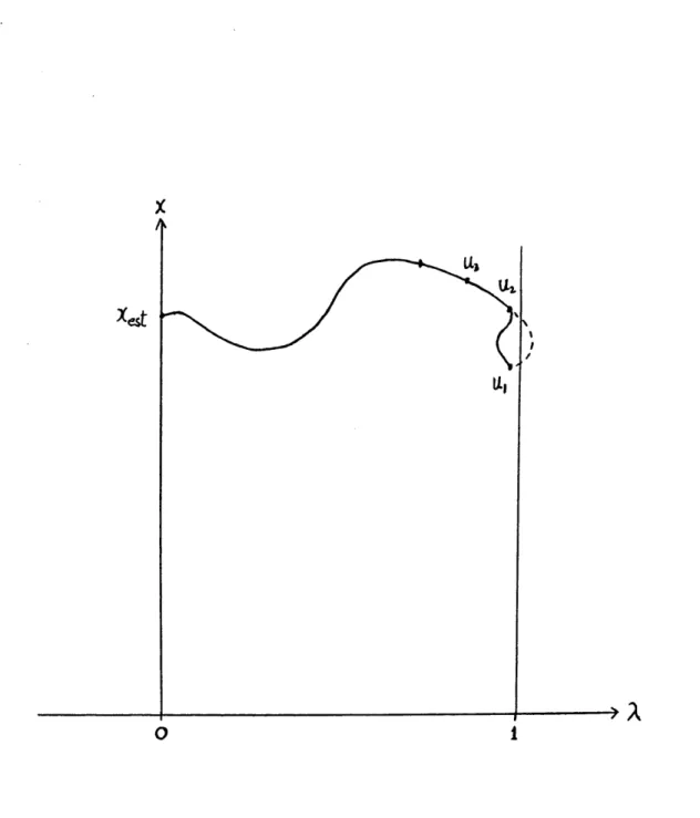
There are two conceivable situations that could cause problems with this scheme. ~ne possibility is that the interpolated curve between Ul and U2 crosses the

A

= 1

hyperplane, but the solution curve does not. For example, see figure 3-5. This situation would lead to a failure to converge in the corrector sub-algorithm. If this happens, the last curve point, Ul, is discarded,

os

is halved and and a new Ul is

computed.

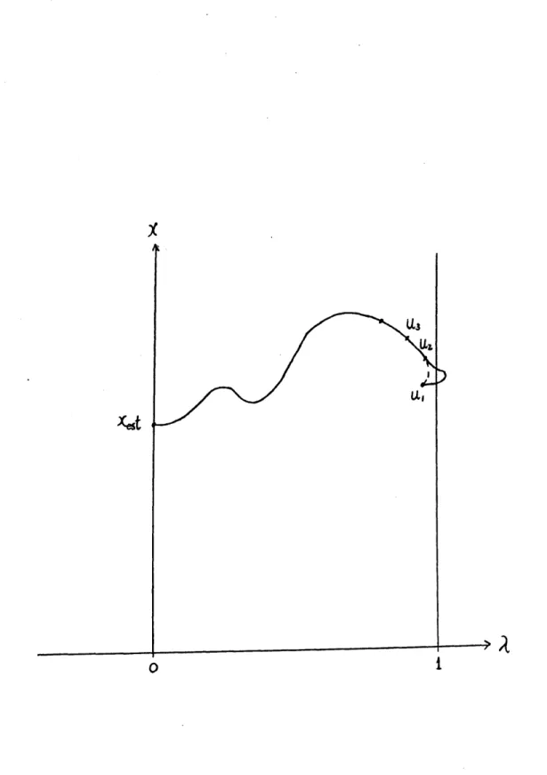
The other potential problem occurs if the solution curve crosses the A == 1 hy-perplane, but the interpolated curve does not. The result of this would be that the algorithm would continue without having recorded a solution point where a solution

xest

lJ.,

o

1

Figure 3-5: Schematic Diagram Showing Potential Problem With Solution State Col-lector

Xest

o

i

Figure 3-6: Schematic Diagram Showing Another Potential Problem With Solution State Collector

point exists. See figure 3-6. Actually, two exact solutions will fail to be recorded. Thankfully, this situation must be extremely rare. If the user checks the critical points (see next section) and finds that there is a critical point with

A

equal to a tiny bit more or less than 1, then he/she should check the possibility that this situation may have occurred.

3.8

Critical State Collection

As mentioned in the previous chapter, the critical states are those points on the solution curve which are local extrema in

A.

The reason for wanting to determine and record such states is related to the possibility of finding that the solution loop on which your a priori estimate lies, and the solution loop on which the solution which we seek lies, are not the same. There is an extended version of this homotopy continuation method that is entirely global. That is, it can follow all existing loops, not just the one on which the a priori estimate lies. Time did not permit the inclusion of that extension in this thesis, but some detailed description of the extension is included in Smith's paper

[1].

A critical state collector was included in this thesis because initially, it was hoped that there would have been time to tackle the extended method. Also,

if

anyone should ever want to add the extension to this piece of work, they would have available a working critical point collector.

The first step of this sub:.algorithm is to check, for

AI,

A2 and A3 corresponding to the last three points on the solution curve, whether either of the following two conditions exist.

If neither of these two conditions exists, it is assumed that there are no local extrema in

A

between Ul and U3. If the first condition exists, it is assumed that there is a

that there is a local maximum in A between U1 and U3'

If it has been determined that a critical point does exist, the task of locating it is carried out. It should be pointed out that the location technique used in this thesis is quite different from the one suggested by Smith

[1].

The location process starts by calculating the arc length in the range [S1' S3] for

which the derivative of A with respect to arc length, on the quadratic Lagrange in-terpolated curve, is equal to zero. This value of arc length is denoted by Seztrm'

It

is

as-sumed that the critical point lies within the restricted range defined bySeztrm:!: 0.2( S1-S3)' The s value corresponding to the +ve sign is denoted by Shigh, and the s value

corresponding to the -ve sign is denoted by Slow. The purpose of this first step is to

reduce the range in which the critical point lies to 40% of the original range. The Lagrange interpolation formulae are used to find approximate points on the solution curve at Shigh, Slow and Seztrm' These three approximate points are then corrected

using the corrector sub-algorithm to give the points on the solution curve denoted by

U'ow, Ueztrm and Uhigh. The arc lengths associated with these points are then corrected

using the arc length corrector sub-algorithm. From this point the location technique consists of a series of reductions of the range of arc lengths, defined by [Shigh, Slow],

within which the critical point lies. When this range is reduced to the point where

Shigh - Slow

<

0.01, and where

I

A

high -

A

,ow

1<

1.0 e-7, then the critical point is

equated to Uellttrm, a point between Uhigh and U'ow'

Each range reduction step involves the following:

• Compute an arc length half-way between Slow and Shigh and call that arc length

Snew •

• Use the Lagrange interpolator to approximate a point on the solution curve at

Snew'

• Correct that point using the corrector sub-algorithm to a point on the solution curve, UneW'

• According to the relative values of .Ahigh, .A'ow, .Anew and .Ae:drm, discard either

Uhigh or U'ow• Reset the other three to Uhigh, U'ow and Ueztrm and repeat the

process until the criteria on arc length and .Aare satisfied.

If the critical point is a maximum, four scenarios for discarding a point and reset-ting the other three exist. They are outlined in figure 3-7. In the first scenario shown the process is : Ueztrm -+ Ueztrm

U'

ow -+

U'

ow Uhigh -+ discarded In the second it is : Uhigh -+ Uhigh Ulow -+ discarded In the third it is : Uhigh -+ Uhigh Ulow -+ discarded In the fourth it is : Unew -+ Ueztrm Ueztrm -+ Uhigh Ulow -+ Ulow Uhigh -+ discarded

x

x

x

x

Figure 3-7: Schematic Diagrams Representing the Different Discard and Reset Sce-nanos

. NOT E :

When a critical point has been determined it is compared with the critical points that have already been recorded. If it is found to be the same as one of the already recorded critical points, that message is recorded instead of recording the same critical point again. The same is true of collection of the solution states. This kind of occurrence indicates either a doubling back of the algorithm, or a situation in which the terminator has failed to recognize a return to the initial start point causing the solution loop to be followed twice. Neither of these things should happen, but at least if they do, there will be evidence to show that they have.

3.9

Termination of the Algorithm

Termination of the algorithm may occur in one of three different ways. The solution loop can be completed, i. e. , the algorithm followed the loop from the initial point, all the way around and back to the initial point. This will be called normal termination. Prior to the completion of the loop, the step size selected may become less than some specified tolerance .. If that happens, the user will be offered the option of terminating. This is an example of optional termination. Prior to the completion of the loop, termination may occur, for example, due to the number of solution points exceeding some maximum allowed number. This is referred to as abnormal termination.

3.9.1

Normal Termination

The normal termination sub-algorithm is very similar to the solution state collector scheme. First it is determined whether the loop has crossed the" = ~hyperplane (in the solution state collector the A = 1 hyperplane was the one of interest). If it has, the exact points at which that occurs are determined in an identical manner to that used in the solution state collector. Now, instead of storing the

A

==

0 states, this sub-algorithm compares them with the initial starting point. If a A

==

0 state is found to be identical to the initial starting point to within some tolerance, then it is clear that the loop has been completed, and the algorithm undergoes normal termination.

3.9.2

Optional Termination

There are two circumstances under which termination is offered as an option to the user. The one which is more likely to occur is that the step size becomes less than some tolerance (1.0 e-5 in this case). This can happen if, for example, the algorithm reaches a part of the solution loop which has hyperbolic orbit states on it. Since the orbit propagation subroutines used in this thesis are only designed to be able to handle elliptic orbits, this will cause the corrector to fail, and therefore the step size to be halved, until the step size is less than the tolerance value. The less likely possibility that leads to optional termination is that the number of stored critical points becomes equal to some specified maximum (10 in this case).

In either case, the options that are offered are :

1. terminate algorithm

2. restart algorithm at the original start point

3. restart algorithm at the last corrected point on the solution curve

If step size is the reason for the options being offered, restarting at the last cor-rected point is not recommended because either the algorithm just runs right back into the same problem that caused the step size to be so small in the first place, or it heads off along the path that it took to get there. That is, the restart causes a doubling back of the algorithm. Restarting at the initial start point may be useful in some cases.

If the number of critical points is the reason for the options being offered, any of the options may prove useful.

3.9.3

Abnormal Termination

One situation that causes the algorithm to terminate prior to completing the solution loop without option, is that the number of solution points recorded exceeds a set maximum number (10 in this case). Other situations which can lead to this kind of termination are :

• Program crashes. Hopefully, this never happens

!!

• Starter step fails either at the very beginning or after a restart option has been chosen. If it happens at the very beginning it is indicative of a probable bug in the software. Otherwise, it is probably due to the situation mentioned in the section on optional termination. That is, where even the tiniest step leads to a point that represents a hyperbolic orbit .

• Normally,

if

the corrector sub-algorithm fails when called from the solution state collector sub-algorithm or from the normal terminator sub-algorithm, the last corrected point is discarded, the step size is halved, and the algorithm continues. However,

if

this happens just after having restarted, the algorithm- terminates.

Details of the Newton-Raphson

Corrector Scheme

The major computational step in the method is the corrector step. This chapter describes that step in detail.

As was indicated in the previous chapter, the corrector sub-algorithm takes a predicted state and corrects it to a state on the solution curve using a Newton-Raphson iterative scheme. Each iteration involves solving a seven-by-seven linear system to get a

ou

correction to the latest prediction. That system is represented by equation 3.4 and equation 3.10 which are reproduced here for convenience.

du

-

.6u

= 0

ds

Since the Yed and Yea:vectors are constants which are specified near the beginning

of the algorithm, the only quantities that remain to be calculated at each iteration are:

1. The set of ranges f(x) IX=Xprl!d computed by propagating the last predicted state.

This will suitably be denoted by Ypred.

epoch orbital elements

f'(x)

IX=Xp,.d. This will suitably be denoted by ~. The

pred subscript has been dropped from the y and the x for clarity, although the

reader should keep in mind that strictly speaking they should be there.

3. The tangent vector ~~.

The range at a given time t after epoch is calculated from the epoch elements by first propagating the epoch elements, x, to that time to get the current elements,

Xt, using whichever dynamics model was chosen (this thesis employs either two-body

mechanics or Brouwer-Lyddane), then by converting those current elements to a satel-lite position in inertial Cartesian coordinates. Finally, knowing the station position in inertial Cartesian coordinates it is simple to calculate the range between station and satellite. Thus, carrying out this process using the last predicted state as epoch, and using the six measurement times, we arrive at the required ranges ypred.

The calculation of the matrix of partial derivatives ~ is more complicated. One method is to evaluate the partial derivatives analytically. The technique used is to calculate them one row at a time. The nth row of the matrix, denoted by 8~~) , where

is calculated from the product of three matrices as follows :

(4.1)

The pv denotes the vector of current position and velocity in Cartesian coordinates. Thus, 88Pvrepresents the six-by-six matrix of the partial derivatives of current position

Xt

and velocity with respect to current elements. A subroutine called CRTDRV [7], which calculates this matrix, provided that equinoctial elements are being use~, was already available.

The row vector,

1~~

,

which represents the partial differentiation of the nth range

as :

Also, let the current station position be represented by :

Then we can express y(n) as :

Simple differentiation thus leads to :

8y(n)

=

(P:Z: -

T:z: py - Ty pz - Tz

0 0 0)

8pv y(n) , y(n) , y(n) , , ,

The relationship between current and epoch equinoctial elements, under the two-body mechanics system, is simply given by :

Pt = P qt

=

q

mt=m+t#

where 1L is the gravitational parameter of the Earth and t is the time elapsed since epoch. Therefore there are only seven non-zero entries in the matrix ~ - six 1'6 on the diagonal and an entry in the bottom left corner given by

-~t#.

The value of

t 'will depend on which row is being computed. 1 0 0 0 0 0 - 0 1 0 0 0 0 0 0 1 0 0 0 0 0 0 1 0 0 0 0 0 0 1 0

_'Jtfj

_{2 a&} 0 0 0 0 1

Theref~re, analytical evaluation of ~ is a good technique for two-body mechanics propagation.

If instead Brouwer-Lyddane propagation is being used, then the relationship be-tween current and epoch equinoctial elements is much more complicated than for two-body mechanics. We can take one of three approaches with Brouwer-Lyddane. We can pretend that the effect of Brouwer-Lyddane on the partial derivatives is neg-ligible, since the only difference between Brouwer-Lyddane and two-body mechanics is that Brouwer-Lyddane includes the first four harmonic terms in the gravity field expansion. Taking this approach we can leave the calculation of partial derivatives in the same form as it was for two-body mechanics. This is the approach suggested by Smith [1]. The second approach is to try to calculate the partial derivatives ana-lytically from the Brouwer theory .. This is intellectually more satisfactory but a great deal of work for possibly little gain. The third approach, which is more of an engineer-ing compromise approach, is to compute the partial derivatives in

*

by numerical differencing.

The second approach was ruled out because of the amount of time it would have taken to develop a subroutine that calculates analytical partial derivatives for the Brouwer-Lyddane propagation model. Both the first and the third approaches were tried and the results compared. The first approach requires substantially less com-putation per step but gives less accurate partial derivatives than the third approach. The effect of the less accurate partial derivatives is generally to cause the algorithm to require smaller step sizes along the curve and consequently to require more steps

to complete the loop. In fact, I found that in areas where the curve had a small radius of curvature the step size was often reduced to a value smaller than the mini-mum allowed and so the algorithm terminated without completing the loop, whereas using numerically determined partials allowed completion of the loop. Based on this finding, I chose to implement the numerical differencing method of calculating partial derivatives for the Brouwer-Lyddane propagation model.

The method of evaluating ~ by numerical differencing is also a row by row process. We start with the set of six ranges

which have been computed by propagating the predicted epoch state

(remember the Fed subscript has been dropped from both y and x), to the six

obser-vation times

To compute :~~~)' the mth entry of the nth row of the partial derivative matrix ~,

propagate the epoch element vector formed by adding 5z{m) to z{m) entry in x, to the

time t{n). Then calculate the resulting range y{re.). The desired entry is given by :

5z(m) should be some very small value and should also be scaled according to which

component of x is being dealt with for the same reason that the

6s

in the starter scheme needed to be scaled. In this thesis ox(m) is equal to 1.0 e-8 times the relevant scaling factor.

Finally, we need to address the calculation of the tangent vector, ~~. One way of calculating the tangent vector is to use the derivatives of the Lagrange interpolating formulae of equations 3.1 and 3.2. This method is discussed in the previous chapter in

the section on the arc length corrector sub-algorithm, and the relevant equations are equation 3.12 and equation 3.13. This is the method used by Smith [1], but he does recommend a second and better method. Initially, in this thesis, the first method was implemented. Later on however, the switch was made to the second method, and it was indeed found to perform better. That second method is outlined as follows.

Differentiation of equation 3.3 with respect to arc length s leads to :

dA

ar

dx

(Ye:r: - Ye.d ds - ax . ds

=

0

Also, in the limit,

ou . ou

=

(OS)2,

which implies:

(

dA):.I

_ds

+

(dX . dX)

_ds

_ds

= 1

(4.2)

(4.3)

If we let the 6-by-1 column vector,

(Ye:r: - Yeat),

be represented by c, and we let the 6-by-6 Jac.obian matrix, :~, be represented by

B,

then equation 4.2 may be written as :

=>

dA

dx

c--B-=O

ds

ds

dx

=

B-1cdA

ds

ds

(4.4)

Substituting equation 4.4 into equation 4.3 gives:

Thus, letting D be defined by :

we can write :

du

=

(dA, dX)

=

(.!-,

B-1C)

This is the expression used in computing the tangent vector at each iteration. Note that Band c have already been computed at this stage so that this tangent evaluation method involves only one non-simple step, i. e. , inverting the B matrix.

In summary, each iteration in the corrector sub-algorithm consists of :

1. Solving the linear seven-by-seven system for

S>' Sz(l) Sz(2) Su= SZ(3) Sz(4) SZ(5) SZ(6)

2. Adding Su to the previous u approximation to get the updated approximation

3. Testing the updated approximation against the convergence criterion

The system is written explicitly as :

SA 0

SZ(I) >.[y(l) _ y(l)] _ y(l)

+

y(l)

e.t ell: e.t

6Z(2) A[y(2) _ y(2)] _ y(2)

+

y(2)

ed ell: e.t

A

SZ(3) _- >.[y(3) _ y(3)] _ y(3)

+

y(3)

ed ell: ed

Sz(4) A[y(4) _ y(4)] _ y(4)

+

y(4)

ed ell: ed

SZ(5) A[y(5) _ y(5)] _ y(5)

+

y(5)

elf e:z: eat

SX(6) A[y(6) _ y(6)] _ y(6)

+

y(6)

where

8>'

8.

(y(l) _ y(l»)_{ez ed}

(y(2) _ y(2»)ez e.t

(y(3) _ y(3»)ele ed

(y(4) _ y(4»)ez e.t

(y(S) _ yeS»)_{ez ed} (y(6) _ y(6»)ez ed 8Z(I} lh _ 8!1~1~ 8z 1 _ 8!1~'~ 8z 1 _ 8!1~3~ 8z 1 _8J4}

a;m

_ 8y~lI~ 8z 1

_ 8yfS~

8z 1 8z('} lh _ 8!1~1~ 8z' _ 811~'~ 8le ' _ 8y~3~ 8z' _ 8y~4~ 8z' _ 8y~lI~ 8z' _ 8!1~6~ 8z' 8Z(3} lh _ 8Jl}

a;m

_ 8Y~'~ 8z3 _ 8y~3~ 8z3 _ 8y~4~ 8z3 _ 8y(lI~ 8z(3 _ 8y~6~ 8z 3 8Z(4} {h _ 8Jl}

a;m

_ 811~'~ 8z4 _ 8y~3~ 8z4 _ 8!1~4~ 8z4 _ 8y(lI} 8z(4) _ 8y~6~ 8z 4 8Z(II} {h _ 8y~l~ 8zII _ 8y~'~ 8z II _ 8J3}

a;m

_8J4}

a;m

_ 8y(lI~ 8z(1I _ 8!1~6~ 8zII 8Z(6}

a;-_ 8y~l~ 8z8 _ 8Y~'~ 8z8 _ 8y~3~ 8z8 _8J4} &fiT _ 8y~lI~ 8z6 _ 8Jl~6~ 8z 8

The actual solving of the linear system is carried out efficiently using a triangular factorization of the

A

matrix, followed by a simple back-substitution scheme. FORTRAN subroutines LUDCMP and LUBKSB used for these two steps are taken from reference [4]. These same subroutines are also used for inverting the B matrix in the tangent evaluation step - equation 4.5.

The final issue related to the corrector sub-algorithm that remains to be discussed, is the convergence criterion. Smith [1] actually employs two criteria and defines the scheme to have converged if either is met. The first is a criterion on the size of the correction vector

Suo

That is, the scheme has converged if

ISul

<

1.0 e - 13

Under certain circumstances it is possible to have a tiny correction vector without actually being very close to the solution. For a simple 2-D example, see figure 4-1.

Thus, this criterion is not so good and has been left out of the present implementation. The other criterion that Smith uses, which is retained in this thesis, is a criterion on the residue of the system of equations. It is written explicitly in the following equation:

.x

Figure 4-1: Simple 2-D Example Showing Why a Convergence Criterion on the Size of the Correction Vector can be Poor

where the maximum is over n.

This criterion can only be satisfied

if

the predicted point is virtually a point on the solution curve.

Chapter

5

Problems With the Algorithm

This chapter is concerned with the various problems associated with the use of the curve following algorithm. The problems are sub-divided into two categories:

• Problems which result in algorithm failure .

• Problems which cause inaccurate solutions to be produced.

The expression algorithm failure needs to be defined here.

Algorithm failure will be defined as any case in which the algorithm terminates before completing the solution loop. This definition allows for the algorithm to fail but yet produce the desired solution state. If by the time the algorithm terminates prematurely, a

A

= 1 state has been recorded, this may already be the desired solution.

There is another problem that can occur which has been mentioned before, but which shall not be discussed in this chapter. That is the problem of completing the solution loop without getting the desired solution. The solution locus is dependent upon the a priori estimate and the distribution of observation times. If either of these is poorly chosen, the solution loop on which your a priori estimate lies may have no

,\ =

1hyperplane crossing points, or it may have some ,\

=

1hyperplane crossing points none of which are the desired solution. An example is discussed as case

#3

in chapter 7. This means that the desired solution lies on a different solution loop to the one on which your a priori estimate lies. The way to overcome this problem is to use the extended method of Smith [1].

5.1

Algorithm Failure

Algorithm failure is very rare when two-body mechanics is the chosen propagation method. In fact, in none of the many real cases that was run with the two-body mechanics propagator did algorithm failure occur. However, there are possible situa-tions which can lead to algorithm failure even with two-body mechanics propagation formulation that was used. One such situation is the existence of epoch states cor-responding to hyperbolic orbits on the solution curve. GTDS subroutine BROLYD was used for both twobody and Brouwer-Lyddane propagation in this thesis. This subroutine is unable to handle parabolic or hyperbolic orbits. If the algorithm reaches a point on the solution curve corresponding to a hyperbolic orbit, the c~rrector step will return to the main algorithm with a non-convergence condition. This in turn will cause the step size to be halved, a new prediction to be made, and the corrector to be tried again. The corrector will repeatedly return a non-convergence condition because the propagator cannot deal with eccentricity> 1. Eventually, the step size will become smaller than the minimum allowed value. At that point, the user will be offered the options of either terminating, restarting at the last corrected point, or restarting at the initial start point in the opposite direction to the one originally chosen. As explained in the section on optional termination in chapter 3, choosing to restart at the last corrected point is not worthwhile under these conditions. There is a formulation of the propagation equations which allows smooth transition between elliptic, parabolic and hyperbolic orbits. This will be discussed in the last chapter.

Fortunately, the existence of hyperbolic solution points on the solution curve is unlikely to occur if the algorithm is being used to determine very low eccentricity orbits and if the chosen a priori estimate also has a low eccentricity. It was noted in the introduction that the Landsat orbits have very low eccentricity, of the order

.1.0 e-3.

Another possible situation that could cause algorithm failure even with two-body mechanics propagation is the situation where there is a bifurcation point on the solution curve. That is, the solution curve is precisely at the transition point of

splitting into two loops. This situation is discussed in the first section of chapter 2, schematically illustrated by figure 2-2, and is very unlikely in practice. The shape of the solution curve is dependent, amongst other things, on the a priori estimate chosen (as equation 2.4 indicates). To demonstrate how unusual it would be to have this happen in a real case, I took some real data and varied the epoch estimate very slowly through a transition point; I was never able to get termination due to existence of a bifurcation point. The plots in figure 5-1 of semi-major axis vs ,\ show how the solution curve shape changed as the epoch estimate was varied through a transition point. The first plot was produced using the following epoch estimate:

a

=

7077.8 km e

=

0.001

i

=

1000 w

=

200

W

=

800 m = 1300

The epoch estimates used to produce the second, third, fourth and fifth plots were identical except that the semi-major axes were respectively 7076 km, 7074.238 km, 7074.237 km and 7070 km. These plots indicate that for an epoch estimate with some semi-major axis between 7074.237 km and 7074.238 km, the solution curve may have a bifurcation point.

If the user is unlucky enough to choose an epoch estimate which produces a bifurcation point on the solution curve, the algorithm would reduce the step size near the bifurcation point until it is smaller than the allowed minimum. At that point, the three options mentioned above will be offered.

A good strategy for deciding which option to take when these three are offered is

0:Utlined as follows :

1. Check the solution points that have been stored up to the point when the options are offered. If an acceptable solution has already been stored then the obvious choice would be to terminate. Otherwise, continue down this list.

..

--/

..•

,,)

.•..

\:

/ i I I

I

/~ /

'\

/

\

I \ / \ I \ .'1.1 ~.5''- o~ ,~ _'l!

_A

.'..

-

~

..

'--

o~ ,~ _a~

A

,'s..cJ.Q, 1 '~ •..clT Q., : _I ~

..

''''''' /~

/

,~

Figure 5-1: Plots Showing the Changing Shape of a Solution Curve as the A Priori Epoch Estimate is Varied in a Real Case