Building improved risk stratification models for patients post non ST-segment elevation acute coronary syndrome using ambulatory ECG data

Building Improved Risk Stratification Models for Patients Post Non ST-Segment Elevation Acute Coronary Syndrome Using Ambulatory ECG Data

by Harlin Lee

S.B., Massachusetts Institute of Technology (2016)

Submitted to the Department of Electrical Engineering and Computer Science in Partial Fulfillment of the Requirements for the Degree of

Master of Engineering in Electrical Engineering and Computer Science

at the MASSACHL

OF TE MASSACHUSETTS INSTITUTE OF TECHNOLOGY

AUG

May2017 (

LIB

0 2017 Harlin Lee. All rights reserved.

The author hereby grants to M.I.T. permission to reproduce and to distribute publicly paper and electronic copies of this thesis document in whole and in part in any medium

now known or hereafter created.

Signature redacted

14

2017

RARIES

ARCHIVES

Department of Electrical Engineering and Computer Science May 25, 2017

Certified by ....

A ccepted by ...

Collin M. Stultz Professor of Electrical Engineering and Computer Science and Professor of Health Sciences Technology Thesis Supervisor

Signature redacted

...

A

Abstract

Accurately and promptly assessing a patient's risk of future adverse cardiovascular events is crucial to the care of patients with non-ST-segment elevation acute coronary syndrome (NSTE-ACS). Inpatient telemetry data are collected for patients post-NSTE-ACS as part of the standard protocol, but current practices do not take advantage of those data to improve the assessment of the patient's long-term risk. Furthermore, previously developed risk metrics that use long-term electrocardiogram (ECG) data focus on instantaneous heart rates and do not fully exploit the ECG morphology, including the clinically important ST-segment morphology. Using a dataset of more than 4400 patients with NSTE-ACS, we developed a logistic regression model that uses the age of the patient and the mean and variance of the level of ST-segment over a 24-hour period, and found that it is highly predictive of one-year cardiovascular death, outperforming other models based on existing ECG-based risk metrics (AUC: 0.761; p<0.001). Uni- and multivariate analysis shows that the model provides information for risk stratification of NSTE-ACS patients beyond what is provided by risk metrics routinely used in clinical

settings, such as TIMI risk score, B-type natriuretic peptide, and left ventricular ejection fraction (adjusted hazard ratio for one-year death (95% Cl): 5.25 (1.42, 21.2)). This model is unique in its simplicity, as it relies on simple logistic regression with only three features, which are automatically computed and easily interpreted. Our findings highlight the prognostic value of subtle ST-segment deviations that fall below the resolution of the human eye.

Introduction

Cardiovascular disease is the leading cause of death in the United States, accounting for 30.8% of all deaths in 2013 (Mozaffarian, Benjamin et al. 2016). Coronary artery disease (CAD), in particular, accounted for one out of every seven deaths in the United States in 2013 (Mozaffarian, Benjamin et al. 2016). CAD is associated with the narrowing and hardening of the coronary arteries, and once it causes an abrupt reduction in blood flow to the myocardium, a patient may suffer a set of clinical conditions called acute coronary

syndrome (ACS).

Patients who have had an ACS are at an increased risk of suffering from adverse cardiac outcomes, such as myocardial infarction (MI) or cardiovascular death (CVD), soon after the diagnosis is made. While great progress has been made in the diagnosis and treatment of patients with an ACS, the rate of CVD in these patients remains unacceptably high.

Based on whether ST-segment elevation is noted in their presenting electrocardiogram (ECG), patients with ACS are classified as having either ST-segment elevation ACS (STE-ACS) or non-ST segment elevation ACS (NSTE-ACS) (Amsterdam, Wenger et al. 2014). Patients with NSTE-ACS, which comprise up to 70% of ACS patients, have varying degrees of atherosclerosis, and therefore varying degrees of risk. Accurate quantification of a NSTE-ACS patient's risk of future adverse cardiovascular events allows health care providers to assign therapies that are appropriate for a given patient's level of risk. Patients who have a high risk of CVD, for example, benefit from invasive therapies (such as surgery or angioplasty) that may lower their risk of death. By contrast,

of subsequent adverse events (Winter and Tijssen 2012) (Mehta, Cannon et al. 2005). The process of grouping patients by their level of risk is called risk stratification, and forms a central component of the management of patients after a NSTE-ACS.

Several models have been developed to aid in risk stratification. The Global Registry of Acute Coronary Events (GRACE) and Thrombolysis In Myocardial Infarction (TIMI) scores are two widely used tools for the NSTE-ACS population, and utilize a mixture of patient demographics, medical history, biomarker data, and ECG data on admission (Granger, Goldberg et al. 2003), (Antman, Cohen et al. 2000). One of the primary advantages of these risk scores is their simplicity, making them easy for clinicians to use. However, commonly used metrics such as these fail to capture a significant number of CVDs in patient populations that are not traditionally considered to be high-risk (Liu,

Syed et al. 2014). Thus, methods with greater discriminative ability are needed.

The standard protocol for caring for patients who present with NSTE-ACS includes hospital admission for inpatient treatment monitoring, including inpatient telemetry. Continuous ECG monitoring allows the early identification of ischemia-induced arrhythmias and potentially ischemic episodes themselves. Interestingly, once the patient is discharged, the continuous ECG data that were acquired during their hospital stay are typically not used to improve their risk assessment.

In the present work, we develop methods that can incorporate different types of patient data, yielding metrics that improve our ability to identify high-risk patient subgroups. Central to this endeavor is the use of long-term ECG data that are routinely acquired on patients who have been admitted with a NSTE-ACS. Although a number of risk

stratification methods that use long-term ECG data exist, such as heart rate variability (HRV), deceleration capacity (DC), and heart rate turbulence (HRT), most of these methods focus on analyses of the instantaneous heart rate and consequently do not exploit other features of the ECG tracing that are known to be correlated with patient outcome (Malik 1996) (Bauer, Kantelhardt et al. 2006) (Schmidt, Malik et al. 1999). As previous studies have shown that analyses of the ST-segment have prognostic value, we therefore focus on developing methods that automatically identify and process ST-segments in long-term ECG data (Kaul, Fu et al. 2001) (Savonitto, Ardissino et al. 1999) (Diderholm, Anden et al. 2002). Moreover, the metrics we devise incorporate information from both an automated analysis of ECG tracings as well as information from the patient record. An advantage of these models is their simplicity, as they rely on simple logistic regression techniques and use a small number of simple features. Using a dataset containing more than 4400 patients who were admitted with a NSTE-ACS, we demonstrate that these models outperform existing metrics.

Results

Patient Populations

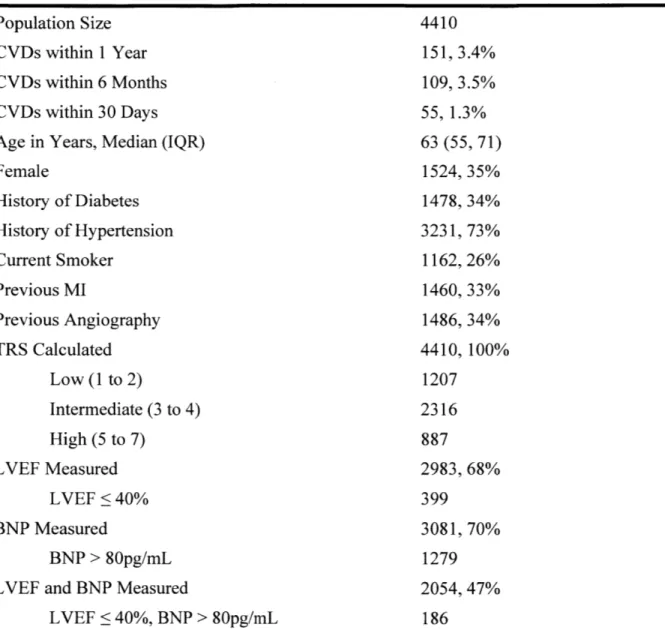
Baseline characteristics of the patients used in this study are presented in Table 1. The patient cohort is a subset of the study population from a clinical study that was used to evaluate the performance of several computational biomarkers in previous works (Morrow, Scirica et al. 2007) (Liu, Syed et al. 2014), (Syed, Stultz et al. 2011), (Syed, Scirica et al. 2009). All patients presented with NSTE-ACS and have at least one day of continuous Holter ECG recordings. The baseline patient features (referred to as "7Hx") consist of seven common risk factors for cardiovascular disease, including age, gender, history of diabetes, history of hypertension, current smoker, previous MI, and previous angiography. ECG Holter data were sampled at 128 Hz.

Logistic Regression Models with Baseline Patient and ECG-Based Features

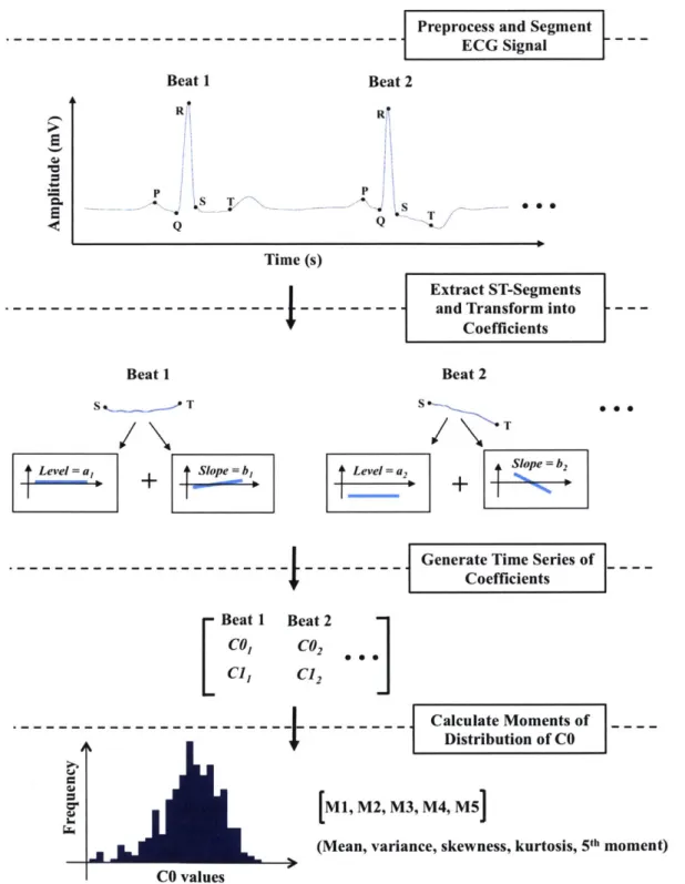
In order to quantitatively model the changes in the morphology of the ST-segment, we used a recently developed mathematical method based on Legendre polynomials (Amon and Jager 2016 .In this approach, the ECG recording for each patient is first segmented into beats and then the ST-segment of each beat is identified and transformed into a set of Legendre polynomial coefficients that capture clinically relevant morphological features. For example, the first coefficient (referred to as "CO") represents the level of the ST-segment relative to the isoelectric line, the second coefficient (referred to as "C11") represents the slope of the ST-segment, and the higher coefficients represent the higher-order curvatures of the ST-segment. We hypothesized that this representation can capture

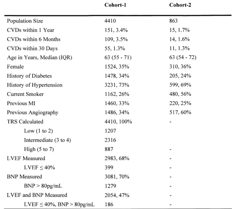
Table 1. Baseline characteristics for the patient cohort. CVD is cardiovascular death; MI is myocardial infarction; TRS is TIMI risk score; LVEF is left ventricular ejaculation fraction; BNP is B-type natriuretic peptide; IQR is interquartile range.

Patient Cohort Population Size

CVDs within 1 Year CVDs within 6 Months CVDs within 30 Days Age in Years, Median (IQR) Female History of Diabetes History of Hypertension Current Smoker Previous MI Previous Angiography TRS Calculated Low (1 to 2) Intermediate (3 to 4) High (5 to 7) LVEF Measured LVEF <40% BNP Measured BNP > 80pg/mL LVEF and BNP Measured

LVEF < 40%, BNP > 80pg/mL 4410 151, 3.4% 109, 3.5% 55, 1.3% 63 (55, 71) 1524, 35% 1478, 34% 3231, 73% 1162, 26% 1460, 33% 1486, 34% 4410, 100% 1207 2316 887 2983, 68% 399 3081, 70% 1279 2054, 47% 186

first explored a model that uses information from both CO and Cl due to the clinical importance of the level and the slope of the ST-segment for the management of ACS. However, we chose to restrict further analysis to CO, as the inclusion of Cl did not lead to any improvement in the prediction of one-year CVD (Table 2).

In this study, we decided to use the central moments of the distribution of CO for each patient to efficiently summarize the prognostic information contained in CO over a 24-hour period. Summarizing the time series in this way has the advantage of producing a small number of features that are easily interpretable and suitable for simple models, such as logistic regression. For every patient in the cohort, we calculated CO for each beat in the first approximately 24 hours of the ECG signal, and then calculated the average CO for every five-minute segment. We then computed the first five central moments (referred to as "CO moments"), namely the mean, variance, skewness, kurtosis, and the fifth normalized central moment, to describe the distribution of CO over all five-minute segments during the 24-hour period (Figure 1). Only the first five moments were included in the model for ease of interpretation.

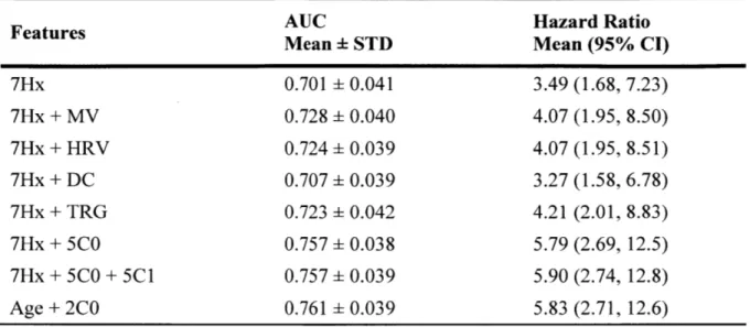
Six logistic regression (LR) models that incorporate patient features were built: a baseline model with only the 7 features derived from the patient's medical history (7Hx), three models that combine 7Hx with an ECG-based risk metric calculated from 24 hours of Holter data, such as MV (Syed, Sung et al. 2009), HRV (Malik 1996), and DC (Bauer, Kantelhardt et al. 2006), a baseline model of 7Hx with TIMI risk score group (TRG) (Antman, Cohen et al. 2000), and a model with the five CO moment features added to the baseline features (7Hx+5C0). Table 2 summarizes the performances of these logistic

Table 2. Performance of 7Hx+5C0 model in predicting one-year CVD. Values represent averages over 1000 bootstrapped trials where each trial yields one AUC, one Hazard Ratio (highest vs. other quartiles) and one 95% Confidence Interval (CI). MV is morphological variability; HRV is heart rate variability LF/HF; DC is deceleration capacity; TRG is TIMI risk score group; STD is standard deviation; AUC is area under the curve.

Features AUC Hazard Ratio

Mean STD Mean (95% CI)

7Hx 0.701 0.041 3.49 (1.68, 7.23) 7Hx + MV 0.728 0.040 4.07 (1.95, 8.50) 7Hx + HRV 0.724 0.039 4.07 (1.95, 8.51) 7Hx + DC 0.707 0.039 3.27 (1.58, 6.78) 7Hx + TRG 0.723 0.042 4.21 (2.01, 8.83) 7Hx + 5CO 0.757 0.038 5.79 (2.69, 12.5) 7Hx + 5CO + 5CI 0.757 0.039 5.90 (2.74, 12.8) Age + 2C0 0.761 0.039 5.83 (2.71, 12.6)

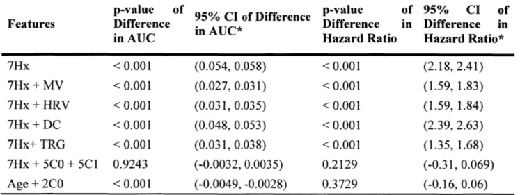
Table S1. Paired sample t-test results between the performance of 7Hx+5C0 performances of remaining models in predicting one-year CVD averaged bootstrapped trials.

model and over 1000

p-value of 95% CI of Difference p-value of 95% CI of

Features Difference in AUC* Difference in Difference in

in AUC Hazard Ratio Hazard Ratio*

7Hx < 0.001 (0.054, 0.058) < 0.001 (2.18, 2.41) 7Hx + MV < 0.001 (0.027, 0.031) < 0.001 (1.59, 1.83) 7Hx + HRV < 0.001 (0.031, 0.035) < 0.001 (1.59, 1.84) 7Hx + DC < 0.001 (0.048, 0.053) < 0.001 (2.39, 2.63) 7Hx+ TRG < 0.001 (0.031, 0.038) < 0.001 (1.35, 1.68) 7Hx + 5C0 + 5C1 0.9243 (-0.0032, 0.0035) 0.2129 (-0.31, 0.069) Age + 2C0 < 0.001 (-0.0049, -0.0028) 0.3729 (-0.16, 0.06) * Difference = (AUC/Hazard logistic regression model)

Preprocess and Segment ECG Signal Beat 2 - 060 R

---

Coefficients Beat 2 S s T t4eel=a, lp=b ST Level = a So b2

Generate Time Series of _

I I Coefficients Beat 1 Beat 2 Col C02 C1, C12 M1, M2, M3, (Mean, varian .K. Calculate Moments of Distribution of CO M4, M5]

ce, skewness, kurtosis, 5th moment) CO values

Figure 1. Overview of the ST-segment feature extraction process. The first five central moments that describe the distribution of the level of ST-segment (Ml, M2, M3, M4, M5) are then inputted into the model along with features chosen from the patient's medical history. Beat 1 R Q 2 Time (s) Beat 1 L

The 7Hx+5C0 model shows a markedly higher AUC compared to the baseline model and all of the other LR models formed by adding an existing ECG-based risk metric to the baseline model (p < 0.001). Besides AUC, one-year univariate hazard ratios (HRs) were calculated using a Cox proportional hazards model (Cox 1972). All six LR models had statistically significant HRs, and improvements in the HR of the 7Hx+5C0 model over the other 7Hx-based LR models were also statistically significant (p < 0.001).

Logistic Regression Model with Reduced Feature Set

Analysis of the weights learned by the 7Hx+5C0 model revealed that the weights associated with age and the first two CO moments (mean and variance) were much larger than those of the other features (Figure 2). These data suggest that a simpler logistic regression model based on only those three features (lHx+2C0) would still be effective. The IHx+2C0 model achieved a mean AUC of 0.761 in predicting one-year CVD over 1000 bootstrapped trials, which was a small but statistically significant improvement to the 7Hx+5C0 model with p <0.001 (Table 2).

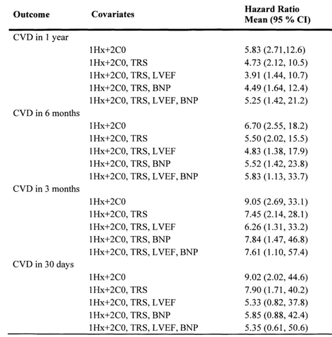
Table 3 shows the results of univariate and multivariate HR analyses done on the 1 Hx+2C0 model over 1000 bootstrapped trials for one-year, six-month, three-month, and 30-day endpoints. When the univariate HRs are adjusted for other clinically used cardiovascular risk metrics, such as the TIMI risk score (TRS), left ventricular ejection fraction (LVEF), and B-type natriuretic peptide (BNP), the HRs of the IHx+2C0 model are still statistically significant for one-year, six-month, and three-month CVD. However, the lHx+2C0 HRs for 30-day CVD are not statistically significant when adjusted for LVEF and BNP.

0~ 0 G31 & 8 0P 619 \0 elk,0

Figure 2. Boxplot of 7Hx+5C0 model weights from 1000 bootstrapped trials of predicting one-year CVD. Red line is median value; blue box edges delineate interquartile range (IQR); red crosses are outliers more than 1.5 IQR beyond box edges; whiskers are minimum and maximum non-outlier values.

- -~ -- _twit - -I-I I I F I II I I 6 4 2 0 -2 -4 -6 -8 C,

Table 3. Univariate and multivariate (TRS, LVEF, BNP) analysis of hazard ratios of the lHx+2C0 model in predicting one-year, 6-month, 9-month, and 30-day CVD. Values are averaged over 1000 bootstrapped trials where each trial yields one Hazard Ratio (highest vs. other quartiles) and one 95% Confidence Interval (CI).

Outcome Covariates Hazard Ratio

Mean (95 % CI) CVD in 1 year CVD in 6 months CVD in 3 months CVD in 30 days 1Hx+2C0 lHx+2C0, TRS IHx+2C0, TRS, IHx+2C0, TRS, IHx+2C0, TRS, 1Hx+2C0 lHx+2C0, TRS IHx+2C0, TRS, lHx+2C0, TRS, IHx+2C0, TRS, 1Hx+2C0 1 Hx+2C0, 1Hx+2C0, lHx+2C0, 1Hx+2C0, lHx+2C0 1Hx+2C0, lHx+2C0, 1Hx+2C0, 1lHx+2C0, TRS TRS, TRS, TRS, TRS TRS, TRS, TRS, LVEF BNP LVEF, BNP LVEF BNP LVEF, BNP 5.83 4.73 3.91 4.49 5.25 6.70 5.50 4.83 5.52 5.83 9.05 7.45 6.26 7.84 7.61 9.02 7.90 5.33 5.85 LVEF BNP LVEF, BNP LVEF BNP LVEF, BNP (2.71,12.6) (2.12, 10.5) (1.44, 10.7) (1.64, 12.4) (1.42, 21.2) (2.55, (2.02, (1.38, (1.42, (1.13, (2.69, (2.14, (1.31, (1.47, (1.10, (2.02, (1.71, (0.82, (0.88, 5.35 (0.61, 18.2) 15.5) 17.9) 23.8) 33.7) 33.1) 28.1) 33.2) 46.8) 57.4) 44.6) 40.2) 37.8) 42.4) 50.6)

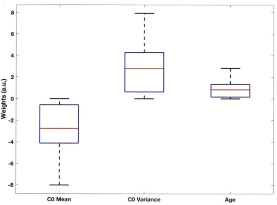
Analysis of the logistic regression weights helps us understand the relative importance of each feature in the prediction model, which was useful in reducing the feature set of the 7Hx+5C0 model to create the lHx+2C0 model. Figure 3 shows a boxplot of the weights learned by the 1 Hx+2C0 model over 1000 bootstrapped trials. A positive (or negative) weight indicates that a higher (or lower) value of the feature is associated with a higher likelihood of one-year CVD; a weight close to zero indicates that the corresponding feature does not contribute much to the model. The positive weight for age is consistent with our knowledge that older patients are at a greater risk for future cardiac outcomes. The negative weights for the mean of CO and the positive weights for the variance of CO seem to suggest that a greater degree of ST-depression and more instability in the level of

8- 6- 4- 2- 0- -2--4 -6 -8

CO Mean CO Variance Age

Figure 3. Boxplot of 1 Hx+2C0 model weights from 1000 bootstrapped trials of predicting one-year CVD. Red line is median value; blue box edges delineate interquartile range; whiskers are minimum and maximum values.

Discussion

Patients with NSTE-ACS are typically admitted for acute management and inpatient monitoring. A central part of monitoring is the routine acquisition of continuous ECG data. While these waveforms are used by health care professionals to diagnose and treat arrhythmia that may occur in the short term, these data are generally not retained nor used to gauge the patient's long-term risk of adverse events. In our view, this represents a lost opportunity as we hypothesize that careful analyses of long-term ECG data can improve our ability to prognosticate. Consequently, we developed a series of logistic regression models that exploit these data to see whether they could identify patients who are at high-risk of death after a NSTE-ACS.

Our work uses an automated analysis of ST-segments that quantifies subtle ST-segment changes over time, which may be difficult to discern by eye. The approach expresses a given ST-segment as a Legendre polynomial expansion, where each term captures a unique feature of the ST-segment. For example, the first coefficient, CO, represents the average value of the ST-segment, the second coefficient, Cl, corresponds to the slope of the segment, the third coefficient quantifies the amount of curvature in the ST-segment, and higher order coefficients capture more subtle morphologic features. Although we initially explored a model that utilized both CO and CI, the results were not significantly improved over models based on data arising from just CO. In our view, this does not necessarily mean that higher order coefficients are not useful. Indeed, the relatively low sampling frequency of our Holter data (128 Hz) means that each ST-segment is modeled with a small number of samples (-16 samples per ST-ST-segment). As

curvature, it is difficult to obtain accurate results with a small number of samples for the underlying signal. Higher sampling rates may therefore be needed to extract meaningful information from higher order coefficients in the expansion.

Using data from only the first Legendre coefficient, we were able to build models that identify patients at elevated risk of CVD after a NSTE-ACS. We found that the 1 Hx+2C0 model, a logistic regression model using age and the mean and variance of CO over a 24-hour period, is highly predictive of CVD among NSTE-ACS patients, outperforming other models based on existing ECG-based risk metrics. Uni- and multivariate analysis revealed that the model provides information for risk stratification of NSTE-ACS patients beyond what is provided by risk metrics routinely used in clinical settings, such as TRS, BNP and LVEF. The IHx+2C0 model is unique in its simplicity, as it relies on simple logistic regression with only three features, which are easily acquired and interpreted.

As we can see from the performances of lHx+2C0 and 7Hx+5C0, adding more features to a model does not necessarily improve its performance. In fact, reducing the feature set from 12 to 3 improved the model's discriminative ability (p <0.001), because we eliminated the 6 patient features and the 3 higher order central moments of CO that, compared to the small amount of prognostic information they were providing, were introducing a lot more noise to the data that the model could overfit to. Similarly, the weights learned by the baseline model with only 7Hx features (Figure Si) show that the eliminated 6 features contribute very little compared to age. These data suggest that these extra risk metrics may not be as useful in risk stratifying patients who have already presented NSTE-ACS.

+ 6 - -4 - 3--0 - + --4-

t

Age Female Diabetes Hypertension Smoker Prior MI Prior Angio

Figure Si. Boxplot of 7Hx model weights from 1000 bootstrapped trials of predicting one-year CVD. Red line is median value; blue box edges delineate interquartile range (IQR); red crosses are outliers more than 1.5 IQR beyond box edges; whiskers are minimum and maximum non-outlier values.

The improvement in AUC of the 7Hx+5C0 model over the 7Hx baseline model is consistent with the improvements in AUC that result from adding other ECG-based metrics to the baseline model. However, the additional improvement in AUC of the

7Hx+5C0 model cannot be explained by the use of long-term ECG data in feature

extraction, since the CO moments, MV, HRV, and DC were all computed from 24 hours of ECG data. The discriminative ability of the 7Hx+5C0 model can be attributed to the ability of CO to capture subtle ST-segment deviations that fall below the resolution of the human eye. We believe that CO makes use of an appropriate amount of ECG morphology; HRV and DC only use instantaneous heart rates and do not take advantage of the detailed morphology, while MV is calculated from the entire beat morphology and does not focus on specific, clinically relevant features. Our results indicate that simple models using relatively small sets of features can offer discriminative ability equal or superior to more sophisticated methods given an appropriate choice of features.

This study has its limitations. The ECG signals were sampled at 128 Hz, and we relied on an automated labeling algorithm for ECG beat segmentation. This study does not show if the results would generalize well to different sampling rates and different segmentation algorithms, but since this model only relies on the mean value of the ST-segment and also the summary statistics of CO from thousands of beats, we expect the 1Hx+2C0 model to be relatively robust.

Materials and Methods

Experimental Design

We used data from a clinical trial that included 4986 post-NSTE-ACS patients with continuous ECG data (Morrow, Scirica et al. 2007). Continuous ECG monitoring was done for one to seven days following randomization with a three-lead digital Holter monitor at a sampling rate of 128 Hz. We eliminated patients who did not have a complete set of the following seven common risk factors for cardiovascular disease (7Hx): age, gender, history of hypertension, history of diabetes, current smoker, prior myocardial infarction, and prior angiography. The patient cohort used to develop and test our models consists of 4410 patients who met these criteria.

To allow for a fair comparison of weights learned by the models, all patient features, including age, MV, HRV, DC, and TRG, were min-max normalized, i.e. linearly scaled by subtracting the minimum and dividing by the range of each feature such that, the values fall in [0, 1].

ECG Preprocessing and Segmentation

The ECG signals were preprocessed as outlined in (Syed, Sung et al. 2009). We eliminated baseline wander by applying a moving average filter of one second to the raw signal, then subtracting the result from the signal. A Daubechies 5 wavelet filter was applied to the resulting signal to reduce high frequency noise, and the Physionet Signal Quality Index package was used to remove noisy beats (Li, Mark et al. 2007). We then

Delineating the waveforms of each beat of the ECG signal was done using a wavelet-based algorithm developed by (Martinez, Almeida et al. 2004) and implemented by (Demski and Llamedo 2016). The algorithm took as input the preprocessed ECG signal and returned a set of labels for the beginning and end of each waveform in each beat. The ST-segment was defined as the set of samples between the end of the S-wave and the beginning of the T-wave. For each ST-segment, we found the midpoint and extracted 16 samples around it for subsequent analysis so that there will be some tolerance to small errors in the labels of the endpoints of the ST-segment. Initially, we excluded beats that contained ST-segments with fewer than 16 samples, more than 32 samples, or were missing a label at the beginning, end, or both the beginning and the end of the ST-segment, because those beats were assumed to be too noisy. However, only a small number of beats passed these criteria.

We then observed the following for each criterion. Most beats without the labels for the beginning of the ST-segment or with ST-segments longer than 32 samples were indeed too noisy; however, many beats without the label for the end of the ST-segment or with ST-segments that were 8 to 15 samples long were actually suitable for feature extraction. Furthermore, we noticed that the algorithm often incorrectly assigned the beginning of the segment a couple samples too early, notably distorting the morphology of the

ST-segment by including parts of the S-wave. To address these issues, we applied the following simple heuristic: if the algorithm detected the beginning of the ST-segment of a beat but missed the end, or if the detected ST-segment was between 8 and 16 samples long, we reassigned the end of the ST-segment to be 19 samples after the beginning of the ST-segment. The value 19 was chosen to be slightly larger than 16 such that the

irm

middle section of the ST-segment that is used for feature extraction would not include the S-wave morphology. In the process, this introduced parts of the T-wave to some of the ST-segments, but since most ECG signals in the cohort had very prominent S-waves and relatively flat T-waves, we decided that this would not significantly misrepresent the morphology of the ST-segment. This heuristic allowed us to recover many usable beats that were originally discarded; there was a median increase of 148% in the number of beats per patient that were included in the analysis.

ST-Segment Morphology Feature Extraction

For each patient, we applied the preprocessing and segmentation steps described above to approximately 24 hours of ECG data. We then applied Gram-Schmidt orthonormalization to the extracted ST-segments to produce a time series of 16 Legendre polynomial coefficients (Amon and Jager 2016). We decided to use only the first coefficient in this study (referred to as "CO"), because it represents the level of the ST-segment, which is routinely examined by clinicians to determine the presence of ischemia. CO was also considered to be most robust to the high frequency noise in the ECG signal, since it represents the average of the 16 sample values in the ST-segment.

We then divided the ECG signal into five-minute segments, which is consistent with the approaches of HRV and MV, and calculated the average of CO for each segment. Five-minute segments that included fewer than 60 ST-segments were discarded, as they were assumed to be too noisy to be used. As a result, we used a median of 23.75 hours of data per patient and an interquartile range of (20.08 - 24.75). Then from the resulting time

first five central moments, i.e. mean, variance, skewness, kurtosis, and fifth standardized moment.

Logistic Regression Models

All logistic regression models presented in this study were trained three times with Li-regularization, with L2-Li-regularization, and without regularization; however, only the results from the regularization scheme that gave the highest mean AUC values are reported in this study. When trained with regularization, three-fold cross-validation was used to determine the best regularization parameter among 25 values.

The main baseline model only included the seven patient history features (7Hx), while four other models had MV, HRV, DC, and TRG in addition to 7Hx. The TRG was defined as 1 for patients with a TRS of 1 to 2, 2 for patients with a TRS of 3 to 4, and 3 for patients with a TRS of 5 to 7. For HRV, we used the HRV LF/HF metric, which corresponds to the ratio of low frequency to high frequency power in the heart rate time series, because this metric was shown to have the greatest predictive power among HRV metrics in our earlier study of patients presenting with NSTE-ACS (Syed, Scirica et al. 2009). The 7Hx+5C0 model had the five CO moments in addition to 7Hx, while 1 Hx+2C0 only included age and the first two CO moments (mean and variance) from the feature set of 7Hx+5C0. Details on how MV, HRV, and DC values were calculated can be found in our previous work (Syed, Stultz et al. 2011).

The performance of each logistic regression model in this study was measured by the AUC and hazard ratio (HR) over 1000 bootstrapped trials. For each bootstrapped trial, the patient cohort was randomly partitioned into a training set of 80% of the data and a testing set of 20%, and each partition was stratified such that the percentage of positive examples was equal in the training and testing sets (-3.4%). The AUC reported for each LR model is the mean of the AUCs over these 1000 runs. HRs were computed using a Cox proportional hazards model, and the upper and lower 95% confidence intervals were calculated by multiplying or dividing, respectively, the HR by the exponentiation of 1.96 times the standard error of the coefficients generated by the Cox model (Cox 1972). The HRs and confidence intervals reported are the mean HRs and the mean of the lower and upper bounds of the 95% confidence intervals over the 1000 trials, respectively. When calculating HRs for each LR model, the high-risk group consisted of patients who are in the upper quartile of risk of experiencing one-year CVD as predicted by the model. When the HRs for the lHx+2C0 model were adjusted for other clinical variables, the high-risk group contained patients based on the following criteria: TRS > 4, LVEF < 40%, or BNP

> 80 pg/mL. (De Lemos, Morrow et al. 2001, Richards, Nicholls et al. 2003) (Richards, Nicholls et al. 2003, Moller, Hillis et al. 2006). Since the percentage of CVDs is quite low in the patient cohort, especially at endpoints earlier than one-year and for the smaller subpopulations for which clinical variables were adjusted, it was necessary to eliminate some of the bootstrapped rounds that contained unusually small numbers of positive examples with which to train and test the models. Except when calculating the multivariate HRs for 30-day CVD, the number of rounds that were eliminated did not

the results significantly. When calculating HRs for 30-day CVD adjusted for BNP, LVEF, and BNP+LVEF, we had to eliminate up to 19% of the rounds. We also tested for statistical significance of the differences in AUCs and HRs between each pair of models by running two-sided, paired-sample (-tests.

All signal processing algorithms, LR models, and statistical analyses were implemented using the commercial software MATLAB 9.1 (2016b) (The MathWorks, Natick, MA).

References

Amon, M. and F. Jager (2016). "Electrocardiogram ST-Segment Morphology Delineation Method Using Orthogonal Transformations." PLOS One.

Amsterdam, E. A., et al. (2014). "2014 AHA/ACC Guideline for the Management of Patients With Non-ST-Elevation Acute Coronary Syndromes." JACC.

Antman, E. M., et al. (2000). "The TIMI Risk Score for Unstable Angina/Non-ST-Elevation MI: A Method for Prognostication and Therapeutic Decision Making." JAMA 284(7): 835-842.

Bauer, A., et al. (2006). "Deceleration Capacity of Heart Rate as a Predictor of Mortality After Myocardial Infarction: Cohort Study." The Lancet 367(9523): 1674-1681.

Cox, D. R. (1972). "Regression Models and Life-Tables." Journal of the Royal Statistical Society, Series B 34(2): 187-220.

De Lemos, J. A., et al. (2001). "The Prognostic Value of B-type Natriuretic Peptide in Patients with Acute Coronary Syndormes." The New England Journal of Medicine 345(14).

Demski, A. and S. M. Llamedo (2016). "ecg-kit a Matlab Toolbox for Cardiovascular Signal Processing." Journal of Open Research Software.

Diderholm, E., et al. (2002). "ST depression in ECG at entry indicates severe coronary lesions and large benefits of an early invasive treatment strategy in unstable coronary artery disease: The FRISC II ECG substudy." European Heart Journal 23: 41-49.

Granger, C. B., et al. (2003). "Predictors of Hospital Mortality in the Global Registry of Acute Coronary Events." ARCH INTERN MED 163: 2345-2353.

Kaul, P., et al. (2001). "Prognostic Value of ST Segment Depression in Acute Coronary Syndromes: Insights From PARAGON-A Applied to GUSTO-IIB." JACC 38(1).

Li,

Q.,

Liu, Y., et al. (2014). "ECG Morphological Variability in Beat Space for Risk Stratification After Acute Coronary Syndrome." JAHA.

Malik, M. (1996). "Heart Rate Variability. Standards of Measurement, Physiological Interpretation, and Clinical Use: Task Force of The European Society of Cardiology and

Martinez, J. P., et al. (2004). "A Wavelet-Based ECG Delineator: Evaluation on Standard Databases." IEEE Transactions On Biomedical Engineering 51(4).

Mehta, S. R., et al. (2005). "Routine vs. selective invasive strategies in patients with acute coronary syndromes: a collaborative meta-analysis of randomized trials." JAMA 293(23): 2908-2917.

Moller, J. E., et al. (2006). "Wall motion score index and ejection fraction for risk stratification after acute myocardial infarction." American Heart Journal 151(2): 419-425. Morrow, D. A., et al. (2007). "Effects of Ranolazine on Recurrent Cardiovascular Events in Patients With Non-ST-Elevation Acute Coronary Syndromes: The MERLIN-TIMI 36 Randomized Trial." JAMA 297(16): 1775-1783.

Mozaffarian, D., et al. (2016). "Executive Summary: Heart Disease and Stroke Statistics

-2016 Update: A Report From the American Heart Association." Circulation 133: 447-454.

Richards, A. M., et al. (2003). "B-Type Natriuretic Peptides and Ejection Fraction for Prognosis After Myocardial Infarction." Circulation 107: 2786-2792.

Savonitto, S., et al. (1999). "Prognostic Value of the Admission Electrocardiogram in Acute Coronary Syndromes." JAMA 281(8).

Schmidt, G., et al. (1999). "Heart-rate turbulence after ventricular premature beats as a predictor of mortality after acute myocardial infarction." The Lancet 353(9162): 1390-1396.

Syed, Z., et al. (2009). "Relation of Death Within 90 Days of Non-ST-Elevation Acute Coronary Syndromes to Variability in Electrocardiographic Morphology." American Journal of Cardiology 103(3): 307-311.

Syed, Z., et al. (2011). "Computationally Generated Cardiac Biomarkers for Risk Stratification After Acute Coronary Syndrome." Science Translational Medicine 3(102). Syed, Z., et al. (2009). "Spectral Energy of ECG Morphologic Differences to Predict Death." Cardiovasc Eng 9(1): 18-26.

Winter, R. J. d. and J. G. P. Tijssen (2012). "Non-ST-Segment Elevation Myocardial Infarction: Revascularization for Everyone?" JACC: Cardiovascular Interventions 5(9): 903-905.

Appendix I. Additional results

Table 1. Baseline patient characteristics for Cohort-I and Cohort-2. CVD is cardiovascular death; MI is myocardial infarction; TRS is TIMI risk score; LVEF is left ventricular ejaculation fraction; BNP is B-type natriuretic peptide; IQR is interquartile range. Cohort-1 Cohort-2 Population Size CVDs within 1 Year CVDs within 6 Months CVDs within 30 Days Age in Years, Median (IQR) Female History of Diabetes History of Hypertension Current Smoker Previous MI Previous Angiography TRS Calculated Low (1 to 2) Intermediate (3 to 4) High (5 to 7) LVEF Measured LVEF < 40% BNP Measured BNP > 80pg/mL LVEF and BNP Measured

LVEF < 40%, BNP > 80pg/mL 4410 151, 3.4% 109, 3.5% 55, 1.3% 63 (55 - 71) 1524, 35% 1478, 34% 3231, 73% 1162, 26% 1460, 33% 1486, 34% 4410, 100% 1207 2316 887 2983, 68% 399 3081, 70% 1279 2054, 47% 186 863 15, 1.7% 14, 1.6% 11, 1.3% 63 (54 - 72) 310, 36% 205, 24% 599, 69% 480, 56% 220, 25% 517, 60%

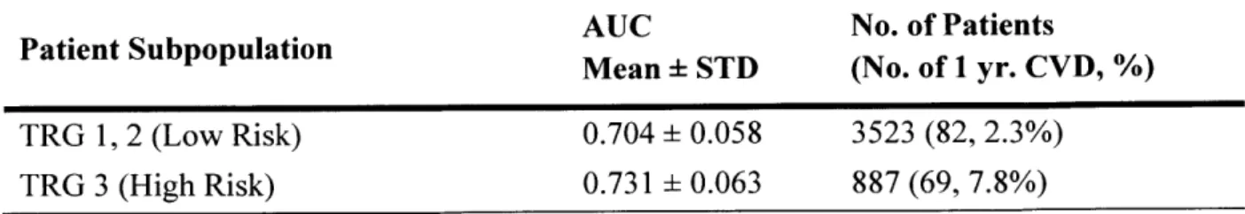
Table 2. Performances of IHx+2C0 model in predicting one-year CVD in subpopulations of Cohort-I over 1000 bootstrapped trials. TRG is TIMI risk score group; AUC is area under the curve; STD is standard deviation.

AUC No. of Patients

Patient Subpopulation _{Mean STD (No. of 1 yr. CVD, %)} TRG 1, 2 (Low Risk) 0.704 0.058 3523 (82, 2.3%)

Table 3. Univariate analysis of hazard ratios of 1Hx+2Cf model predicting one-year, 6-month, and 30-day CVD in low-risk patients of Cohort-I with TRG < 3.

Outcome Hazard Ratio No. of Inf HRs

Mean (95 % CI)

CVD in I year 4.18 (1.49, 11.8) 0

CVD in 6 months 4.88 (1.40, 17.7) 0

Table 4. Performances of logistic regression models in predicting one-year CVD in Cohort-i over 1000 bootstrapped trials. STDEP1 is ST-depression greater than 1mm at presentation; TRG is TIMI risk score group; STD is standard deviation; AUC is area under the curve.

Features AUC Mean STD TRG lHx 2C0 7Hx + TRG == 3 7Hx + TRG lHx + 2C0 + TRG 7Hx + STDEP1 IHx + 2C0 + STDEP1 0.671 0.041 0.696 0.043 0.731 0.042 0.720 0.041 0.723 0.042 0.766 0.040 0.746 0.038 0.773 0.038

0.07 -- High-Risk Group - Low-Risk Group 0.06-

0.05-

Figure 1. Kaplan-Meier curve for Cohort-2 (cutoff= 75th percentile of Cohort-I rounded to one digit). lHx+2C0 model is trained on Cohort-i and tested on Cohort-2. High-risk group has 18 patients and 1 death. Univariate hazard ratio is 3.69 (0.48, 28.2). Model scores for calibration, median (IQR): Cohort-i is 0.031 (0.023 -0.041), Cohort-2 is 0.014

Table 5. Net Reclassification Improvement (NRI) from 7Hx+5C0 model to 1Hx+2C0 model. NRI is calculated by averaging results from 1000 bootstrapped trials in Cohort- 1.

Total NRI Event NRI Non-Event NRI

Types of NRI Mean STD Mean STD Mean STD

Continuous -0.014 0.63 -0.004 0.49 -0.010 0.18

Category-based (Cutoff _{is 0.0015 0.06 0.0010 0.06 0.0005} 0.01 75th percentile of training set)

Category-based (Cutoff _{is 0.0037 0.06 0.0036 0.06 0.0001 0.00} 75th percentile of test set)

Table 6. Univariate and multi7arintA (TRS, BNP) analysis of hazivA

rat;os

lHx+2C0+STDEP1 predicting one-year, 6-month, and 30-day CVD in Cohort-1.

Outcome Covariates Hazard Ratio No. of

Mean (95 % CI) Inf HRs CVD in 1 year lHx+2C0+STDEP1 6.43 (2.95, 14.1) 0 lHx+2C0+STDEP1, TRS 5.19 (2.29, 11.8) 0 IHx+2C0+STDEP1, TRS, LVEF 5.20 (1.82, 15.3) 0 lHx+2C0+STDEP1, TRS, BNP 4.88 (1.70, 14.3) 0 IHx+2C0+STDEP1, TRS, LVEF, BNP 6.84 (1.69, 30.4) 4 CVD in 6 months lHx+2C0+STDEP1 7.54 (2.78, 21.4) 0 IHx+2C0+STDEPl, TRS 6.22 (2.20, 18.4) 0 lHx+2C0+STDEP1, TRS, LVEF 6.81 (1.75, 29.6) 3 lHx+2C0+STDEP1, TRS, BNP 6.48 (1.55, 30.4) 3 IHx+2C0+STDEP1, TRS, LVEF, BNP 8.32 (1.45, 53.2) 52 CVD in 30 days lHx+2C0+STDEP1 9.28 (2.08, 45.8) 12 IHx+2C0+STDEP1, TRS 8.08 (1.73, 41.5) 12 lHx+2C0+STDEP1, TRS, LVEF 7.24 (1.02, 55.3) 101 lHx+2C0+STDEP1, TRS, BNP 7.81 (1.07, 61.3) 109 lHx+2C0+STDEP1, TRS, LVEF, BNP 7.77 (0.83, 77.1) 367

8 6 4 2 0 -2 -4 -61| -A

CO Mean CO Variance Age STDEP1

Figure 2. Boxplot of lHx+2C0+STDEP1 weights over 1000 bootstrapped trials of predicting one-year CVD in Cohort-1. Red line is median value; box edges are interquartile range; whiskers are minimum and maximum values.

Table 7. Performances of 1 Hx+2C0 in prediating one-year CVD in Cohort-3 over 1000 bootstrapped trials with varying amount of ECG data used in feature extraction. bpm is beats per minute. (Cohort-3: 4330 patients in Cohort-1 with 24*3600 clean beats, 145 (3.4%) one-year CVD)

Amount of ECG Data Used

(Length in Time if Heart Rate is Constantly 60 bpm) 60 beats (1 minute) 300 beats (5 minutes) 3600 beats (1 hour) 3*3600 beats (3 hours) 6*3600 beats (6 hours) 12*3600 beats (12 hours) 18*3600 beats (18 hours) 24*3600 beats (24 hours) AUC Mean STD 0.736 0.042 0.738 0.042 0.742 0.042 0.748 0.042 0.752 0.041 0.754 0.041 0.755 0.041 0.755 0.040

Table 8. Paired sample t-test results over 1000 bootstrapped trials between the performances of 1 Hx+2C0 models in predicting one-year CVD in Cohort-3 with varying amount of ECG data used in feature extraction.

p-value of 95% CI of

ECG Used in Model 1 ECG Used in Model 2 Difference in Difference in

AUC AUC*

300 beats (5 min) 60 beats (1 min) < 0.001 (0.0012, 0.0017) 3600 beats (1 hr) 300 beats (5 min) < 0.001 (0.0037, 0.0044) 3*3600 beats (3 hrs) 3600 beats (1 hrs) < 0.001 (0.0062, 0.0069) 6*3600 beats (6 hrs) 3*3600 beats (3 hrs) < 0.001 (0.0031, 0.0036) 12*3600 beats (12 hrs) 6*3600 beats (6 hrs) < 0.001 (0.0017, 0.0022) 18*3600 beats (18 hrs) 12*3600 beats (12 hrs) < 0.001 (0.0007, 0.0011) 24*3600 beats (24 hrs) 18*3600 beats (18 hrs) 0.8965 (-0.0034, 0.0038) 24*3600 beats (24 hrs) 60 beats (1 min) < 0.001 (0.015, 0.022)

Appendix II. Documentation of codebase and datasets

Every file needed to reproduce the results of this project can be found in one of the three following places: the c3ddbOl.mit.edu server, "Stultz ECG Project" Dropbox folder, and a 4TB backup hard drive in lab.

Original datasets and files

from

The original MERLIN (Cohort-1) dataset is hosted in borg-login-i .csail.mit.edu. Once you are given access to the folder, you can access it using the following commands: ssh

{{username}}@borg-login-1.csail.mit.edu -i {{location of rsa private

key in your local machine}} and cd /data/ddmg/data/merlin. The raw ECG

files are saved as ORGANIZED/{{patientID}}/{{dayNum}}/{{dayNum}}.mat, and

patient records are saved in META/xx2.mat, as described in META/merlinvars.txt. Folders ORGANIZED/{{patientID}}/{{dayNum}} also include files generated from the MV project.

The original DISPERSE (Cohort-2) dataset is hosted in ddmgl.csail.mit.edu, and it can be accessed by the following remote access command: ssh

{{username}}@ddmgl.csail.mit.edu -i {{location of rsa private key in

your local machine}} and cd /archive/ddmg/data/timi. The DISPERSE

ORGANIZED folder is structured similarly to the MERLIN ORGANIZED folder.

Project folder in c3ddb0l.mit.edu server

ssh {{username}}@c3ddb0l.mit.edu -i {{location of rsa private key in

your local machine}} and cd /scratch/users/harlin/ecgdelineation/. Run

is to see the list of folders and files present in the directory. Folders merlinfinal/{{patientID}} contain the corresponding patient's raw ECG signals

({{dayNum}}.mat), and the beat segmentation labels

({{patientID}}_day{{dayNum}}_wavedetnew2.mat) from MERLIN. Similarly,

timi/ORGANIZED/{{patientID}} folders contain the raw ECG signals and their segmentation labels from DISPERSE.

The folders si and sltimi have files in the format of

slrr_{{patientID}}_day{{dayNum}}.mat. Inside the file, each column of the

variables sl and rr correspond to a beat that passed the heuristics described in Methods. The 16 rows of sl correspond to the 16 Legendre polynomial coefficients (CO, Cl,

C 15); the first row of rr is the index of the R peak, and the second row of rr is the length

of the RR interval, both in number of samples.

All features used in the logistic regression models are saved in the slrrfeatures

folder. Different files in data have CO and Cl calculated using ECG data from different days of the clinical trial. Of particular interest are these two files: data/slhralldayl.mat used approximately 24 hours of ECG data from MERLIN, and data/sl_hr_timi-dayl.mat used approximately 24 hours of ECG data from DISPERSE. Within each of those files, each row of the variables represents a patient, whose ID can be found in ids. Each column represents the averaged value over a 5-minute window; hrs is heart rate, slo is CO, and sli is Cl.

The actual features that are inputted into the models are in the s1 moTes f ~ ~ ~ ~ ~ X~~~~~~~~~~~~~~ XXIL4& %L4LL1 ~ ~ ~ IU l 1IF LUII% 11,I~JAaG% II LII. IL_ o en - ROI I. "I1 l I particular, the results presented in this work are from using

slmoments/c0_moments dayl.mat (MERLIN) and

slmoments/cOmoments idaytimi.mat (DISPERSE). Within each file, each of the 4410 and 863 rows of a variable represent a patient from Cohort-i and Cohort-2, respectively. The logistic regression models use the slmoments variable to predict y. sl moments has the first five CO moments (in order: mean, variance, skewness, kurtosis, 5th normalized central moment) and the seven patient record features (in order: age, female, diabetes, hypertension, smoker, prior MI, prior angiography) in each column, min-max normalized, and y has one-year CVD and patientlD in each column.

The results of running 1000 bootstrapped trials on MERLIN using these features are

saved in LRresults. The filenames are formatted as LRresults/{{features used}}_{{optional additional descriptors}}_LRresults_{{timestamp}} .mat.

Each of these files include the X and Y that were inputted, as well as results, a Matlab

struct object with three structs for each regularization (NR, i.e. no regularization, L1, L2).

Each of these structs have vectors of length 1000, where each value is from one

bootstrapped trial; aucs is AUC, hr_lr is hazard ratio, bs is weights, and cihrlr is

confidence interval of hazard ratio. AUCs reported in this work are calculated by

mean(aucs) std(aucs), and hazard ratios (95% CI) by mean(hr_lr)

(mean(hrlr./cihr_lr), mean(hr-lr.*cihr_lr)). The hazard ratios have 13

rows for univariate and multivariate analysis results: 1 for just model score (LR), 2 for LR + TRG, 3 for LR + TRG + LVEF, 3 for LR + TRG + BNP, and 4 for LR + TRG +

All Matlab codes written during the course of this project are located in the st_code folder. Each of them are commented, and describes the expected input and output in the beginning, so this section should only be used as a guide to navigate the stcode folder; for detailed instructions, please read the actual code file. Note that the ECG segmentation codes will only work after installing the ecg-kit package as described in the link (http://marianux.github.io/ecg-kit/).

File Name Function Description

Returns the moving average for a given signal and window slidgavg_mex.csize.

Daubechies 5 wavelet filters a given signal. Used to reduce high frequency noise in ECG signals.

Saves ECG signal into a .mat file with appropriate headers a wthat can be recognized by ecg-kit.

Loads the file outputted from prepare wavedet.m, and calls ecg-kit functions to label waveforms of the signal.

Calls preparewavedet and runwavedet_vl for each

hour--n- qlong ECG segment.

Applies the ST-segment heuristics, and combines different

fixstlabel.m files outputted from runwavedet_ql.m to

* wavedetnew2.mat.

Calculates Legendre polynomial coefficients (CO, Cl, etc) using ECG signal and *_wavedetnew2.mat.

Calculates average HR, CO, and CI for every 5-minute t g sr _{window for each patient. Outputs data/slhrall_*.mat.}

Calculates CO moments, and combines them with patient sanitize_sl_moments. m

history features to make slmoments/cOmomentsday1.mat. Runs 1000 bootstrapped trials to train and test logistic --lc- _{regression models. Calculates AUC and hazard ratios.}

The ddb.k11L.UU cluster uses L11 SLUVM workload manager (https://slurm.schedmd.com/) to schedule jobs. To submit a job to the cluster, read the instructions in the link and refer to codes in the slurmcode folder for guidance.

Dropbox folder

The "Stultz ECG Project" Dropbox folder has sirrfeatures, LRresults, and stcode.

Backup hard drive

The 4TB backup hard drive, physically located in lab, has merlin-final, si, si_timi, sirrfeatures, LRresults, and st_code.

Acknowledgements

I want to thank my thesis advisor, Professor Collin Stultz, for holding my hand through the project and helping me grow as a researcher, a student, and a person. I would also like to thank those in my lab, especially Paul Myers and Yun Liu, for their support and helpful discussions, as well as Professor John Guttag, Jen Gong, Jeff Ashe from GE, Dr. Maulik Majmudar, and Professor Charlie Soudini for their input during our regular research meetings. I should also mention my friends and family who were so kind to let me complain to them about this project all year; in particular, Puppycat, the past and present Safetyfourth & Eurah, the legendary Media Lab Wine Club, friends in Next House (Safetythird), and Senior Haus (206). And of course, my family for supporting my pursuit of science and knowledge.