Beyond Keywords
The MIT Faculty has made this article openly available.
Please share
how this access benefits you. Your story matters.
Citation
Houghton, James P., Michael Siegel, Stuart Madnick, Nobuaki
Tounaka, Kazutaka Nakamura, Takaaki Sugiyama, Daisuke
Nakagawa, and Buyanjargal Shirnen. “Beyond Keywords.”
Sociological Methods & Research (October 10, 2017):
004912411772970. © 2017 The Authors
As Published
http://dx.doi.org/10.1177/0049124117729705
Publisher
SAGE Publications
Version
Original manuscript
Citable link
http://hdl.handle.net/1721.1/120723
Terms of Use
Creative Commons Attribution-Noncommercial-Share Alike
Beyond Keywords: Tracking the evolution of conversational clusters
in social media
James P. Houghton
Michael Siegel
Stuart Madnick
Nobuaki Tounaka
Kazutaka Nakamura
Takaaki Sugiyama
Daisuke Nakagawa
Buyanjargal Shirnen
Working Paper CISL# 2016-13
October 2017
Cybersecurity Interdisciplinary Systems Laboratory (CISL)
Sloan School of Management, Room E62-422
Massachusetts Institute of Technology
Cambridge, MA 02142
Beyond Keywords: Tracking the evolution of
conversational clusters in social media
James P. Houghton
1, Michael Siegel
1, Stuart Madnick
1,
Nobuaki Tounaka
2, Kazutaka Nakamura
2, Takaaki Sugiyama
2,
Daisuke Nakagawa
2, and Buyanjargal Shirnen
21
Massachusetts Institute of Technology, Cambridge, MA, USA
2Universal Shell Programming Laboratory Ltd., Tokyo, Japan
October 9, 2017
Abstract
The potential of social media to give insight into the dynamic evo-lution of public conversations, and into their reactive and constitutive role in political activities, has to date been underdeveloped. While topic modeling can give static insight into the structure of a conver-sation, and keyword volume tracking can show how engagement with a specific idea varies over time, there is need for a method of analy-sis able to understand how conversations about societal values evolve and react to events in the world, incorporating new ideas and relat-ing them to existrelat-ing themes. In this paper, we propose a method for analyzing social media messages that formalizes the structure of public conversations, and allows the sociologist to study the evolution of public discourse in a rigorous, replicable, and data-driven fashion. This approach may be useful to those studying the social construc-tion of meaning, the origins of facconstruc-tionalism and internecine conflict, or boundary-setting and group-identification exercises; and has po-tential implications for those working to promote understanding and intergroup reconciliation.
1
Motivation
Social media suggests a tantalizing prospect for researchers seeking to
un-derstand how newsworthy events influence public and political conversations.
Messages on platforms such as Twitter and Facebook represent a high
vol-ume sample of the national conversation in near real time, and with the
right handling
1can give insight into events such as elections, as
demon-strated by [Huberty, 2013, Tumasjan et al., 2010]; or processes such as social
movements, as demonstrated by [Agarwal et al., 2014,DiGrazia, 2015].
Stan-dard methods of social media analysis use keyword tracking and sentiment
analysis to attempt to understand the range of perceptions surrounding these
events. While helpful for basic situational awareness, these methods do not
help us understand how a set of narratives compete to interpret and frame
an issue for action.
For example, if we are interested in understanding the national
conver-sation in reaction to the shooting at Emanuel AME church in Charleston,
South Carolina on June 17, 2015, we could plot a timeseries of the volume
of tweets containing the hashtag #charleston, as seen in Figure 1. This
tells us that engagement with the topic spiked on the day of the news, and
then persisted for several days before returning to baseline. It does not tell
us that the initial spike may have been retellings of the details of the event
1The primary issues involve controlling for demographics. For examples of methods for
handling demographic concerns with social media data, see [Bail, 2015, McCormick et al., 2015].
itself, with the tail comprised of interpretations and framings of the event in
the political discourse, the ways the event is interpreted by various groups,
or how these groups connect the event to their preexisting ideas about gun
violence. Additionally, it does not let us track continuing engagement with
the follow-on ideas stimulated by the original discussion.
Figure 1: Standard methods of social media analysis include keyword volume
tracking
3(shown here), sentiment analysis, and supervised categorization
Alternate methods include assessing the relative ‘positive’ or ‘negative’
sentiment present in these tweets, or using a supervised learning categorizer
to group messages according to preconceived ideas about their contents, as
demonstrated by [Becker et al., 2011,Ritter et al., 2010,Zubiaga et al., 2011].
Such methods can give aggregated insight into the sentiment expressed, but
fail to uncover from the data the ways the events are being framed within
existing conversations.
3Data presented here (and in the remainder of this paper) is from a 1% random sample
of twitter messages. The number of messages listed in the y axis of this figure (and other count based figures) represents volume within the sample. For an estimate of the overall volume, multiply by 100.
Because they look at counts of individual messages and not at the
re-lationships between ideas, techniques which focus on volume, sentiment, or
category are unable to uncover coherent patterns of thought that signify a
society’s interpretation of the events’ deeper meanings. To interpret events,
individuals must make connections between an event and historical
paral-lels or concepts in the public discourse. It is thus the expressed connections
between ideas, not merely the ideas themselves, which must be tracked,
cat-egorized, and interpreted as samples from an underlying semantic structure.
Our approach inverts the investigation of structures of connected persons
observed in social networks, as demonstrated by [Zachary, 1977] or [Morales
et al., 2015], and instead investigates structures of connected ideas within
semantic networks.
4While the individual-level semantic networks which constitute personal
interpretation of events are fundamentally unobservable, messages sent by
in-dividuals encode samples of these connections in an observable format. These
individual-level samples can be aggregated to form a societal-level network
representing the superposition of active semantic network connections of the
society’s members. For the purpose of this paper, it is sufficient to note that
if structure is discernible in this aggregate then structure is implied within
the members, allowing that no one individual need represent more than a
subset of the aggregate structure.
54For a theoretical discussion of semantic networks as representations of human
knowl-edge, see [Woods, 1975], [Mayer, 1995] and [Schilling, 2005], for a physiological description see [Tulving, 1972] and [Collins and Quillian, 1969].
One way to aggregate these connections is to look at a network of word
co-occurrences in social media messages, as has been demonstrated by
[Co-gan and Andrews, 2012, Smith and Rainie, 2014]. This technique represents
references to an event, to analogous historical events, and to other public
discourse concepts as nodes in a semantic network. Each message containing
two concepts contributes to the weight of an edge between these nodes. The
structure that results gives a macro-level aggregated sample of the
micro-level structures of meaning within individuals’ own minds. For example,
Figure 2 shows the network of hashtags formed around the focal concept of
the Charleston shooting, on June 18, 2015. Each hashtag in the
conversa-tion is represented as a point or ‘node’ in this diagram, and each message
containing a pair of hashtags contributes to the strength of the link or ‘edge’
connecting those two nodes.
6Within this example appear two distinct clusters of connected ideas. In
this case, the upper cluster represents a description of the shooting itself and
the human elements of the tragedy, and the lower cluster focusses on the
larger national-scale political conflicts to which the event relates. Within
each cluster, ideas relate to one another, and connections give context to
and comment upon one another.
We might consider this the essence of
surprising. One could imagine that such an aggregate would resemble a random network, and the fact that this is not the case suggests an underlying sociological process for the social construction of meaning. A full description of how these processes may operate is forthcoming by the first author.
6Here we use a cutoff threshold to convert a frequency-weighted set of connections into
an unweighted network diagram.
Figure 2: Coherent structures in the aggregate hashtag co-occurrence
net-work can serve as proxies for ‘conversations’ in the larger societal discourse,
and give insight into the structures of meaning within the minds of individual
members of that society
what is meant by a national conversation around a topic - a set of mutually
acknowledged statements of meaning. In contrast, across clusters we see
fewer connections between ideas, suggesting that the statements made within
one cluster do not inform or relate to those from the other. By examining the
structure of the semantic network, we begin to see that instead of one national
conversation reacting to the event, there are (at least) two conversations going
1.1
The contributions of this paper
We may hypothesize that how these conversations evolve and interact will
influence the social and political response to the event they describe. In
this paper we build on the qualitative example above, and present a formal
method for identifying conversational clusters, describing their structures,
and tracking their development over time. We present various methods for
visualizing conversational structure to give insight into how certain elements
form the central themes of a conversation while other elements circulate
on the margins. We show how overlapping conversational clusters may be
identified, and explore their relevance to discussions of factionalism and
con-sensus building. We then demonstrate a method for tracking the evolution
of these conversational clusters over time, in which clusters identified on one
day are compared with clusters emerging on subsequent days. This allows
us to identify how new concepts are being included into the discussion, and
quantitatively track engagement in full conversations as distinct from mere
references to keywords.
Formally representing elements of a conversation as being frequent vs.
rare, or central vs. marginal, and tracking how these metrics develop over
time, allows the sociologist to study the way new ideas obtain relevance. For
example, a central and well-connected topic may become prominent through
a process of amplification, or a related popular topic may become relevant
through a process of linking. These phenomena, which happen societally at
the level of individual terms, can then be studied as drivers of macro-level
phenomena such as factionalism, polarization, and realignment. By tying
the changes in conversation to changes in underlying social structures, the
narrative identity-forming and boundary-setting activities of groups may be
studied.
In the appendices to this paper we provide example scripts that save
those wishing to use these techniques from the burden of reimplementing
these algorithms. Due to the computation-intensive nature of this analysis,
we chose to implement the data manipulation algorithms in both Python and
Unicage shell scripts,
7for prototyping and speed of execution, respectively.
Descriptions of these scripts can be found in the appendices, along with
performance comparisons between the two languages.
2
Identifying Conversation Clusters
The network in Figure 2 represents connections individuals have made
be-tween hashtags.
8Each of the hashtags present in the dataset forms a node
in this network, and the relative strength of edges depends upon the
num-ber of times the pair occur together in a tweet, their ‘co-occurrence’, using
the method of [Marres and Gerlitz, 2014].
9To formally identify the
clus-7For a description of Unicage development tools, see [Tounaka, 2013]
8The attributes of these connections are not considered in this analysis, and may thus
be positive or negative, binding or exclusive.
9It is of course possible to conduct the analysis using the full set of words present in
a tweet, omitting stop-words, or focussing purely upon easily identifiable concepts. From an analytical perspective, this has the effect of expanding the scale of the clusters, as a broader range of concepts are included. Within this paper, we limit the analysis to hashtags purely for the purposes of simplifying the presentation, and keeping visualizations to an
ters visually present in the diagram, we apply k-clique community detection
algorithms, implemented in the COS Parallel library developed by [Gregori
et al., 2013] and demonstrated in the appendices.
Clique percolation methods work to identify communities of well-connected
nodes within a network in a way that allows for the possibility of overlapping
or nested communities. The methods allow the analyst to create metrics that
identify communities based upon local network characteristics and are thus
invariant to network size or connectivity outside of the local community. As
the measured extent of a conversation should be determined by the content
and connectivity of that conversation, and not by the structure of unrelated
discussion, this method of community detection is for our purposes superior
to those based upon graph cutting or intersubjective distance measures.
10The K-clique percolation method suggests that communities are
com-posed of an interlocking set of cliques of size k, that is k nodes which are all
mutually connected to each other; and that the overlap of each clique with a
neighboring clique is (k-1). This ensures that each member of a community
is connected to at least (k-1) other mutually-connected nodes within the
community, and that any sub-communities are connected by a bridge of at
appropriate size. We are grateful to an anonymous reviewer for highlighting that a full text analysis not only allows for a larger sample of messages to be observed within the conversation, but is essential for researchers studying how concepts rise to prominence, as the initial process of concept formation or linkage is likely to occur before the concepts are institutionalized with a hashtag. A comparison of the full-text and hashtag-only analysis is present in Appendix F.
10For a comparison of community detection algorithms and their features, see [Porter
et al., 2009].
least width k.
The metric k determines how strict the conditions are for membership in
a cluster, and thus drives cluster extent and boundaries. For example, high
values of k would impose strict requirements for interconnectedness between
elements of an identified conversation, leading to a smaller, more coherent
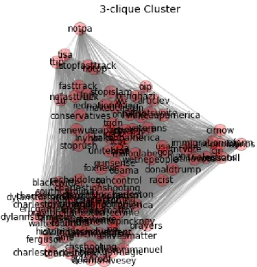
identified conversation, as seen in Figure 3. Each member of this cluster is
connected to at least 4 other members who are all connected to one another.
Figure 3: Clusters with higher k value are smaller and more tightly connected,
representing a more coherent or focused conversation
On the other hand, smaller values of k are less stringent about the
re-quirements of connectivity they put on the elements in the cluster, leading
to a larger, more loosely coupled group as seen in Figure 4, whose members
must be connected to at least two other mutually connected members of the
community.
Figure 4: Clusters with lower k value are larger and less less tightly connected,
representing more diffuse conversation. They may have smaller clusters of
conversation within them
is a collection of sets of words which all form a conversational cluster. As the
extent and connectivity of the identified cluster is dependent upon the value
of k used to create it, by varying k we can identify closely connected subsets
that represent the central structures of the conversation, and occasionally
multiple subsets representing internal factions within the discussion.
As the algorithms depend only on the presence, not the strength of
con-nections within the conversation, information of the volume of messages
mak-ing a semantic connection can be encoded as a threshold weight w for inclusion
into the analyzed co-occurrence network. By varying w we can identify the
extent to which a connection is recognized by members of the population. To
demonstrate the utility of these parameters we explore their extrema.
Clus-ters that form with high values of k and low values of w may be considered
central to the conversation, but only by a minority of the population.
Con-versely, concepts contained only within clusters with high values of w and
low values of k are universally agreed to be marginally related to the focal
discussion.
3
Representing Conversational Clusters as Nested
Sets
Tight conversational clusters (high k) must necessarily be contained within
larger clusters with less stringent connection requirements (lower k).
Per-forming clustering along a range of k values allows us to place a specific
conversation in context of the larger discourse. It becomes helpful to
repre-sent these clusters as nested sets as seen in Figure 5, ignoring the node and
edge construction of the network diagram in order to display the nested and
interlocking relationships the conversations have with one another. In this
diagram, members of a 5-clique cluster are arranged (in no particular order)
within the darker blue box. These form a subset of a larger 4-clique cluster
which also includes a number of other concepts.
With this representation we see elements of the conversation that are
Figure 5: Converting networks to nested sets based upon k-clique clustering
simplifies presentation and analysis of various levels of conversation
relating to one another less tightly. Existing methods which look at volume
may suggest that ideas are central to a conversation if they are well
repre-sented in the sample. These methods lack the ability to analytically discern
that different topics are located within the core of different conversations.
Within the nested structure presented here, central topics are defined not by
their volume, but by the multiplexity of their connection with other concepts
which also form the core of the discussion, elements to which they relate and
whose meaning they are seen as essential to. Within the larger
conversa-tion, peripheral terms are less mutually interdependent, and less essential for
understanding.
Specifically, this method allows the qualitative observation of
conversa-tional clusters that we drew from Figure 2 to be formalized into an explicit
and analytically tractable structure. The upper cluster of our example is
highlighted here, and we show that this cluster is actually composed of a
more tightly connected set of central ideas referencing the event itself and
the immediate response it elicits, embedded within a broader set of ideas
additionally referencing the perpetrator and victims.
11In noting that the
abstractions of terrorism and racism are part of the center of this part of the
conversation, with the specific details closer to the margins, the sociologist
may wonder if this is because the event is seen primarily as an instance of
a more important phenomena than as an interesting occurrence in its own
right.
4
Tracking Conversations Chronologically
In order to track how elements of conversation weave into and out of the
general discourse over time, we need to be able to interpret how
conversa-tional clusters identified at one point in time relate to those in subsequent
intervals. We can do this in one of two ways.
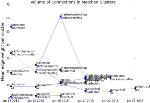
The first method is to track the volume of co-occurrences identified in the
various conversational clusters identified on the first day of the analysis, as it
changes over subsequent days. This indicates how well the connections made
on the first day maintain their relevance in the larger conversation. Figure 6
shows how the connections made in conversational clusters on June 18th fall
in volume over the 10 days subsequent to the initial event, paralleling the
11This also reveals that ideas which at first seem related, such as ‘racism’ and ‘racist’
might hold different valences. This diagram would suggest that systemic racism attributed to the event is more closely connected with other details of the conversation than is its specific manifestation in the racist perpetrator. The robustness of these conclusions would need to be explored by further varying the thresholds used to construct these clusters.
decay in pure keyword volume seen in Figure 1.
Figure 6: Tracking the volume of connections made in a single day’s clusters
(e.g. co-occurrences) reveals how the specific analogies made immediately
after the event maintain their relevance
The second method for tracking conversation volume over time takes into
account the changes that happen within the conversation itself. The
funda-mental assumption in this analysis is that while the words and connections
present in a conversation change, they do so incrementally in such a way as
to allow for matching conversations during one time period with those in the
time period immediately subsequent.
12[Palla et al., 2007] discuss how communities of individuals develop over
time and change. We can use the same techniques to track the continuity of
conversational clusters. The most basic way to do this is to count the overlap
12For an intuitive analogy, consider that a fraction of your favorite baseball team may
be replaced in any given year, but the ‘team’ persists. It would be easy to identify these persisting teams by matching rosters from one season with those from the preceding and subsequent seasons, even if particular players transfer to other teams in the league.
of elements of conversational clusters at time 1 and time 2, as a fraction of
the total number of elements between the two, and use this fraction as the
likelihood that each cluster at time 2 is an extension or contraction of the
time 1 cluster in question. From this we can construct a transition matrix
relating conversational clusters at time 1 with clusters at time 2.
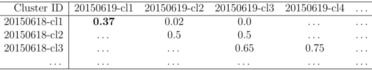
13For instance, if we wish to understand the likelihood that the outermost
cluster illustrated in Figure 5 transitions to a subsequent cluster on June
19th, as visualized in Figure 7, we can count the number of words present
in both days (7: ‘terrorism’, ‘dylannroof’, ‘charlestonshooting’, etc...) and
divide by the total unique number of words in the clusters on both days
combined (19: adding ‘whitesupremacy’, ‘massmurder’, etc...), giving a value
of 0.37.
14This value forms the entry in our transition matrix with row
20150618-cl1, and column 20150619-20150618-cl1, excerpted in Table 1. Other clusters which
are candidates for succeeding our focal cluster form other entries in the same
row. Other clusters from the first day and their candidates for transition
form the additional rows.
13In this analysis, we form clusters using all messages sent on a given day, and look at
transitions from day to day. This is appropriate as the underlying sociological process we are interested in occurs at this timescale. For slower-changing conversations, it may be useful to construct clusters by aggregating messages to the weekly or monthly level, and computing transitions between these times
14To improve our estimates, we can take advantage of the fact that clusters that
corre-spond from time 1 to time 2 will participate in a larger cluster that emerges if we perform our clustering algorithm on the union of all edges from the networks at time 1 and time 2. Omitting entries in the transition matrix which do not nest within this joint cluster reduces the number of possible pairings across days, yielding a sparser and more specific intra-day transition matrix.
Figure 7: A cluster from one day can be related to a cluster on the next day
with likelihood proportional to their shared elements
This transition matrix describes the similarity between a cluster in one
time-period (rows) and a corresponding cluster in the subsequent time-period
(columns). If a cluster remains unchanged from one time-period to the next,
the value at the location in the transition matrix with row index
correspond-ing to the cluster on the first day and column index correspondcorrespond-ing to the
cluster on the second day will be equal to 1. On the other hand, if the
clus-ter breaks into two equal and fully separate groups, each of these will have a
value of .5 in their corresponding column, as for cluster 20150618-cl2 in the
table. When one of the groups is larger than the other, it will be given a
cor-respondingly higher value. If two overlapping clusters form by splitting the
original cluster, their combined values may exceed 1, as for cluster
20150618-cl3, and if significant fractions of the original cluster are not present in any
subsequent cluster, the sum of all values for that row may be less than 1.
We should thus interpret the transition matrix not as a way to select the
single subsequent cluster out of many which represents the original cluster
Table 1: Clusters at t1 have some likelihood of continuing as clusters at t2
Cluster ID
20150619-cl1
20150619-cl2
20150619-cl3
20150619-cl4
. . .
20150618-cl1
0.37
0.02
0.0
. . .
. . .
20150618-cl2
. . .
0.5
0.5
. . .
. . .
20150618-cl3
. . .
. . .
0.65
0.75
. . .
. . .
. . .
. . .
. . .
. . .
. . .
transformed and brought forward in time. Instead the value should be
in-terpreted as the confidence that a subsequent cluster may be considered a
continuation of the original cluster. Thus by looking at the distribution of
values within a row in the transition matrix, we can identify situations in
which a conversation splits, or multiple conversations merge to form a single
larger conversation.
These dynamics point to underlying processes of polarization,
factional-ism, or reconciliation within the population engaging in the discussion. We
should expect that in the process of meaning-making with regards to an
event, the emergence of consensus should be characterized as a move
to-ward fewer clusters as some clusters merge and others fall out of the larger
discussion. Increasing polarization suggests the fission of conversations into
partially overlapping clusters, as individuals from each faction begin to talk
past one another, highlighting different aspects of the overarching
conversa-tion.
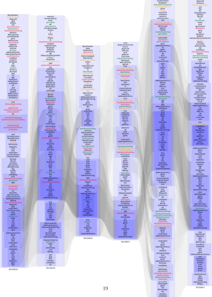
Figure 8: Weighted traces connect conversational clusters as they evolve day
to day
clusters transition from day to day. In Figure 8, weighted traces connect
conversations on June 18th to their likely continuations on June 19th, then
20th, and so on, with heavier traces implying greater continuity from day to
day.
In the first column of this figure, corresponding to June 18, 2015, we see
the conversation illustrated by Figure 5 in the context of a larger conversation
also including preexisting clusters of conservative politics, the 2016 election
cycle, and issues such as gun control and the Trans Pacific Partnership. In
this first day following the shooting, a tight conversational cluster relates
the details of the shooting: the event and its location (‘charlestonshooting’,
‘massmurder’, etc.), the victims (‘clementapinkney’, ‘emanuelame’), and the
perpetrator (‘dylannroof’). These we highlight in red. Using the language
of [Benford and Snow, 2000], we also see words representing early
‘diag-nostic framing’; which define the event as a problem, explain the cause of
that problem, and attribute blame. These we highlight in orange (‘racism’,
‘terrorism’).
In the second column, corresponding to June 19th, concrete details of
the shooting no longer form a tight cluster, but references to the event
(‘charlestonshooting’) become more central to the conversation regarding
conservative politics, suggesting that a process of meaning-making is
under-way. References to existing ‘prognostic’ framings, which articulate
appropri-ate response strappropri-ategies, likewise move more towards the core of the political
These we highlight in green (‘progun’, ‘gunfreezone’, ‘notonemore’).
In June 20, additional references to existing prognostic framings move into
the core of the conversation (‘momsdemand’), and new diagnostic framings
enter the larger conversation as details of the perpetrator’s motivation emerge
(‘confederate’, ‘whiteprivilege’, ‘confederateflag’). As calls are made for the
South Carolina state legislature to remove the Confederate flag from the state
capitol grounds, new prognostic framings enter the discussion (‘takeitdown’,
‘takedownthatflag’). In the fourth column, representing June 21st,
diagnos-tic and prognosdiagnos-tic framings gel together in clusters linking the Confederate
flag to the Charleston shooting and racism, and to the Black Lives Matter
movement. A counterframing (‘alllivesmatter’, ‘gohomederay’) forms its own
overlapping conversational cluster.
On June 22, the shooting itself has become less tightly linked with
politi-cal discussion, as it is replaced with prognostic framings and politi-calls to
solidar-ity actions (‘charlestonstrong’, ‘unsolidar-itychaincharleston’, ‘bridgetopeace’). In
response to political pressure, the Confederate flag is removed from the state
capitol. On June 23rd, the tight clustering of prognostic framing linked with
the references to the shooting has dissipated, and the conversation returns
to its longer-term structure, with movement references again moving toward
the margins of the discussion.
Having explored the way the conversation that was formed in response
to the shooting evolved into a conversation about the state’s support for
symbols of racism, we can finally return to the original task of assessing
public engagement with the discussion.
In figure 9 we show the volume
associated with each of the sub-conversations and some of the key terms
associated with their evolution. Here we observe that in shifting its emphasis
from a conversation about the event alone to a discussion with more political
relevance, overall engagement with the topic actually surpasses the original
discussion about the event on the first day.
This leads to the sociological conclusion that rather than the typical news
cycle, what we see in this case is actually the trigger of a small wave of social
activism linked to a larger social movement.
Figure 9: The average (1% sample) volume of messages in each evolving
cluster shows how engagement with the conversation (as opposed to specific
keywords) varies over time
5
Discussion and Conclusion
Through our analysis, it is clear that the ‘National Conversation on Racism’
that gained steam following the Charleston shooting was not a single
dis-cussion of a single set of issues. By structuring as a semantic network the
way various concepts built and reflected on one another, we recognized that
there may have been be multiple simultaneous but separate conversations
addressing different aspects of the tragedy. By examining the density of
re-lationships within each conversation, we found the central aspects of each
conversation. By tracking the evolution of these conversations over time, we
saw how events became linked to larger social issues, and how these links
drew on prior discussion to frame and suggest responses to the events. These
conclusions can only be drawn by understanding the links between the event
and its interpretations as they evolve over time.
The utility of social media analysis for sociological research can be
ex-tended well beyond the practice of tracking keyword volume, net post
sen-timent, or supervised classification. In particular, tracking conversational
clusters within a network of idea co-occurrences can give both structural
un-derstanding of a conversation, and insight into how it develops over time.
These tools can prove helpful to sociologists interested in using social media
to understand how world events are framed within the context of existing
conversations.
Follow-on work to this paper could attempt to separate the various
versational clusters according to the groups engaged in them, possibly using
information about the Twitter social network to understand if certain
con-versations propagate through topologically separate subgraphs, or if multiple
conversations occur simultaneously within the same interconnected
commu-nities. Such research would have obvious impact on our understanding of
framing, polarization, and the formation of group values.
6
Author’s Note
The appendices to this paper contain all of the code needed to collect
nec-essary data, generate the analysis, and and produce visualizations found
herein:
Appendix A Cluster Identification and Transition Analysis in Python
Appendix B Cluster Identification and Transition Analysis in Unicage
Appendix C Performance Comparison Between Python and Unicage
Ex-amples
Appendix D Data Collection Scripts
Appendix E Visualizations
Appendix F Comparison of hashtags-only analysis with full analysis
The full set of scripts, and associated documentation, can be found at
References
[Agarwal et al., 2014] Agarwal, S. D., Bennett, W. L., Johnson, C. N., and
Walker, S. (2014). A model of crowd enabled organization: Theory and
methods for understanding the role of twitter in the occupy protests.
In-ternational Journal of Communication, 8:646–672.
[Bail, 2015] Bail, C. A. (2015). Taming Big Data: Using App Technology to
Study Organizational Behavior on Social Media. Sociological Methods &
Research.
[Becker et al., 2011] Becker, H., Naaman, M., and Gravano, L. (2011).
Beyond Trending Topics: Real-World Event Identification on Twitter.
ICWSM.
[Benford and Snow, 2000] Benford, R. D. and Snow, D. a. (2000). Framing
Processes and Social Movements : An Overview and Assessment. Annual
Review Sociology, 26(1974):611–639.
[Cogan and Andrews, 2012] Cogan, P. and Andrews, M. (2012).
Reconstruc-tion and analysis of twitter conversaReconstruc-tion graphs. Proceedings of the First
ACM International Workshop on Hot Topics on Interdisciplinary Social
Networks Research.
[Collins and Quillian, 1969] Collins, A. M. and Quillian, M. R. (1969).
Re-trieval Time from Semantic Memory. Journal of Verbal Learning and
Ver-bal Behavior, 8:240–247.
[DiGrazia, 2015] DiGrazia, J. (2015). Using Internet Search Data to Produce
State-level Measures: The Case of Tea Party Mobilization. Sociological
Methods & Research.
[Gregori et al., 2013] Gregori, E., Lenzini, L., and Mainardi, S. (2013).
Par-allel k-clique community detection on large-scale networks. IEEE
Trans-actions on Parallel and Distributed Systems, 24(8).
[Huberty, 2013] Huberty, M. (2013). Multi-cycle forecasting of congressional
elections with social media. Proceedings of the 2nd workshop on Politics,
Elections and Data.
[Marres and Gerlitz, 2014] Marres, N. and Gerlitz, C. (2014).
Interface
Methods: Renegotiating relations between digital research, STS and
Soci-ology.
[Mayer, 1995] Mayer, R. E. (1995). The Search for Insight: Grappling with
Gestalt Psychology’s Unanswered Questions.
In Sternberg, R. J. and
Davidson, J. E., editors, The Nature of Insight, pages 1 online resource
(xviii, 618 p.)–1 online resourc.
[McCormick et al., 2015] McCormick, T. H., Lee, H., Cesare, N., Shojaie,
A., and Spiro, E. S. (2015). Using Twitter for Demographic and Social
Science Research: Tools for Data Collection and Processing. Sociological
[Morales et al., 2015] Morales, A. J., Borondo, J., Losada, J. C., and
Ben-ito, R. M. (2015). Measuring Political Polarization: Twitter shows the
two sides of Venezuela. Chaos: An Interdisciplinary Journal of Nonlinear
Science, 25(3).
[Palla et al., 2007] Palla, G., Barab´
asi, A., and Vicsek, T. (2007).
Quantify-ing social group evolution. Nature.
[Porter et al., 2009] Porter, M. a., Onnela, J.-P., and Mucha, P. J. (2009).
Communities in Networks. American Mathematical Society, 56(9):0–26.
[Ritter et al., 2010] Ritter, A., Cherry, C., and Dolan, B. (2010).
Unsuper-vised modeling of twitter conversations. In Human Language Technologies:
The 2010 Annual Conference of the North American Chapter of the ACL,
pages 172–180.
[Schilling, 2005] Schilling, M. A. (2005). A ”Small-World” Network Model
of Cognitive Insight. Creativity Research Journal, 17(2-3):131–154.
[Smith and Rainie, 2014] Smith, M. and Rainie, L. (2014). Mapping twitter
topic networks: From polarized crowds to community clusters.
[Tounaka, 2013] Tounaka, N. (2013). How to Analyze 50 Billion Records in
Less than a Second without Hadoop or Big Iron.
[Tulving, 1972] Tulving, E. (1972). Episodic and semantic memory.
[Tumasjan et al., 2010] Tumasjan, A., Sprenger, T., Sandner, P., and Welpe,
I. (2010). Predicting Elections with Twitter: What 140 Characters Reveal
about Political Sentiment. ICWSM.
[Woods, 1975] Woods, W. A. (1975). WHAT’S IN A LINK: Foundations for
Semantic Networks. Technical Report November.
[Zachary, 1977] Zachary, W. W. (1977). An Information Flow Model for
Conflict and Fission in Small Groups. Journal of Anthropological Research,
33(4):452–473.
[Zubiaga et al., 2011] Zubiaga, A., Spina, D., Fresno, V., and Mart´ınez, R.
(2011). Classifying trending topics: a typology of conversation triggers on
twitter. Proceedings of the 20th ACM international conference on
This code takes messages that are on twitter, and extracts their hashtags. It then constructs a set of weighted and unweighted network structures based upon co-citation of hashtags within a tweet. The network diagrams are interpreted to have a set of clusters within them which represent 'conversations' that are happening in the pool of twitter messages. We track similarity between clusters from day to day to investigate how conversations develop.
These scripts depend upon a number of external utilities as listed below:
import datetime
print 'started at %s'%datetime.datetime.now()
import json
import gzip
from collections import Counter
from itertools import combinations
import glob
import dateutil.parser
import pandas as pd import os import numpy as np import datetime import pickle import subprocess #load the locations of the various elements of the analysis
with open('config.json','r') as jfile:
config = json.load(jfile)
print config
Appendix A: Cluster Identification and Transition Analysis
in Python
Utilities
We have twitter messages saved as compressed files, where each line in the file is the JSON object that the twitter sample stream returns to us. The files are created by splitting the streaming dataset according to a fixed number of lines - not necessarily by a fixed time or date range. A description of the collection process can be found in Appendix D.
All the files have the format posts_sample_YYYYMMDD_HHMMSS_aa.txt where the date listed is the date at which the stream was initialized. Multiple days worth of stream may be grouped under the same second, as long as the stream remains unbroken. If we have to restart the stream, then a new datetime will be added to the files.
# Collect a list of all the filenames that will be working with
files = glob.glob(config['data_dir']+'posts_sample*.gz')
print 'working with %i input files'%len(files)
Its helpful to have a list of the dates in the range that we'll be looking at, because we can't always just add one to get to the next date. Here we create a list of strings with dates in the format 'YYYYMMDD'. The resulting list looks like:
['20141101', '20141102', '20141103', ... '20150629', '20150630']
dt = datetime.datetime(2014, 11, 1)
end = datetime.datetime(2015, 7, 1)
step = datetime.timedelta(days=1)
dates = []
while dt < end:
dates.append(dt.strftime('%Y%m%d'))
dt += step
print 'investigating %i dates'%len(dates)
The most data-intensive part of the analysis is this first piece, which parses all of the input files, and counts the various combinations of hashtags on each day.
Supporting Structures
weeks, but becomes unwieldy beyond this timescale.
#construct a counter object for each date
tallydict = dict([(date, Counter()) for date in dates])
#iterate through each of the input files in the date range
for i, zfile in enumerate(files):
if i%10 == 0: #save every 10 files
print i,
with open(config['python_working_dir']+"tallydict.pickle", "wb" ) as picklefile:
pickle.dump(tallydict, picklefile)
with open(config['python_working_dir']+"progress.txt", 'a') as progressfile: progressfile.write(str(i)+': '+zfile+'\n')
try:
with gzip.open(zfile) as gzf:
#look at each line in the file
for line in gzf:
try:
#parse the json object
parsed_json = json.loads(line)
# we only want to look at tweets that are in
# english, so check that this is the case.
if parsed_json.has_key('lang'):
if parsed_json['lang'] =='en':
#look only at messages with more than two hashtags,
#as these are the only ones that make connections
if len(parsed_json['entities']['hashtags']) >=2:
#extract the hashtags to a list
taglist = [entry['text'].lower() for entry in parsed_json['entities']['hashtags']]
# identify the date in the message
# this is important because sometimes messages
# come out of order.
date = dateutil.parser.parse(parsed_json['created_at'])
date = date.strftime("%Y%m%d")
#look at all the combinations of hashtags in the set
for pair in combinations(taglist, 2):
#count up the number of alpha sorted tag pairs
tallydict[date][' '.join(sorted(pair))] += 1 except: #error reading the line
print 'd',
except: #error reading the file
We save the counter object periodically in case of a serious error. If we have one, we can load what we've already accomplished with the following:
with open(config['python_working_dir']+"tallydict.pickle", "r" ) as picklefile:
tallydict = pickle.load(picklefile)
print 'Step 1 Complete at %s'%datetime.datetime.now()
Having created this sorted set of tag pairs, we should write these counts to files. We'll create one file for each day. The files themselves will have one pair of words followed by the number of times those hashtags were spotted in combination on each day. For Example:
PCMS champs 3 TeamFairyRose TeamFollowBack 3 instadaily latepost 2 LifeGoals happy 2 DanielaPadillaHoopsForHope TeamBiogesic 2 shoes shopping 5 kordon saatc 3 DID Leg 3 entrepreneur grow 11 Authors Spangaloo 2
We'll save these in a very specific directory structure that will simplify keeping track of our data down the road, when we want to do more complex things with it. An example:
twitter/ 20141116/ weighted_edges_20141116.txt 20141117/ weighted_edges_20141117.txt 20141118/ weighted_edges_20141118.txt etc...
We create a row for every combination that has a count of at least two.
commands as if through a terminal. Lines prepended with the exclaimation point ! will get passed to the shell. We can include python variables in the command by prepending them with a dollar sign $ .
for key in tallydict.keys(): #keys are datestamps
#create a directory for the date in question
date_dir = config['python_working_dir']+key if not os.path.exists(date_dir):
os.makedirs(date_dir)
#replace old file, instead of append
with open(config['python_working_dir']+key+'/weighted_edges_'+key+'.txt', 'w') as fout: for item in tallydict[key].iteritems():
if item[1] >= 2: #throw out the ones that only have one edge
fout.write(item[0].encode('utf8')+' '+str(item[1])+'\n')
Now lets get a list of the wieghed edgelist files, which will be helpful later on.
weighted_files = glob.glob(config['python_working_dir']+'*/weight*.txt')
print 'created %i weighted edgelist files'%len(weighted_files)
print 'Step 2 Complete at %s'%datetime.datetime.now()
We make an unweighted list of edges by throwing out everything below a certain threshold. We'll do this for a range of different thresholds, so that we can compare the results later. Looks like:
FoxNflSunday tvtag android free AZCardinals Lions usa xxx هرﺮﺤﺘﻣ ﺰﻠﺒﻛ CAORU TEAMANGELS RT win FarCry4 Games
We do this for thresholds between 2 and 15 (for now, although we may want to change later) so the directory structure looks like:
twitter/ 20141116/ th_02/
unweighted_20141116_th_02.txt th_03/ unweighted_20141116_th_03.txt th_04/ unweighted_20141116_th_04.txt etc... 20151117/ th_02/ unweighted_20141117_th_02.txt etc... etc...
Filenames include the date and the threshold, and the fact that these files are unweighted edge lists.
for threshold in range (2, 15):
for infile_name in weighted_files:
date_dir = os.path.dirname(infile_name)
date = date_dir.split('/')[-1]
weighted_edgefile = os.path.basename(infile_name)
#create a subdirectory for each threshold we choose
th_dir = date_dir+'/th_%02i'%threshold if not os.path.exists(th_dir):
os.makedirs(th_dir)
# load the weighted edgelists file and filter it to
# only include values above the threshold
df = pd.read_csv(infile_name, sep=' ', header=None, names=['Tag1', 'Tag2', 'count'])
filtered = df[df['count']>threshold][['Tag1','Tag2']]
#write out an unweighted edgelist file for each threshold
outfile_name = th_dir+'/unweighted_'+date+'_th_%02i'%threshold+'.txt'
with open(outfile_name, 'w') as fout: #replace old file, instead of append
for index, row in filtered.iterrows():
try:
fout.write(row['Tag1']+' '+row['Tag2']+'\n')
except:
unweighted_files = glob.glob(config['python_working_dir']+'*/*/unweight*.txt')
print 'created %i unweighted edgelist files'%len(unweighted_files)
print 'Step 3 Complete at %s'%datetime.datetime.now()
We're using COS Parallel to identify k-cliques, so we feed each unweighted edge file into the ./maximal_cliques preprocessor, and then the ./cos algorithm.
The unweighed edgelist files should be in the correct format for ./maximal_cliques to process at this point.
./maximal_cliques translates each node name into an integer to make it faster and easier to deal with, and so the output from this file is both a listing of all of the maximal cliques in the network, with an extension
.mcliques , and a mapping of all of the integer nodenames back to the original text names, having extension .map .
It is a relatively simple task to feed each unweighed edgelist we generated above into the ./maximal_cliques algorithm.
for infile in unweighted_files:
th_dir = os.path.dirname(infile)
th_file = os.path.basename(infile)
#operate the command in the directory where we want the files created
subprocess.call([os.getcwd()+'/'+config['maximal_cliques'], th_file], cwd=th_dir)
maxclique_files = glob.glob(config['python_working_dir']+'*/*/*.mcliques')
print 'created %i maxcliques files'%len(maxclique_files)
print 'Step 4a Complete at %s'%datetime.datetime.now()
current_directory = os.getcwd()
for infile in maxclique_files:
mc_dir = os.path.dirname(infile)
mc_file = os.path.basename(infile)
subprocess.call([os.getcwd()+'/'+config['cos-parallel'], mc_file], cwd=mc_dir)
Step 4: Find the communities
Step 5: Once this step is complete, we then feed the .mcliques output files
into the cosparallel algorith.
community_files = glob.glob(config['python_working_dir']+'*/*/[0-9]*communities.txt')
print 'created %i community files'%len(community_files)
print 'Step 5 Complete at %s'%datetime.datetime.now()
The algorithms we just ran abstract away from the actual text words and give us a result with integer collections and a map back to the original text. So we apply the map to recover the clusters in terms of their original words, and give each cluster a unique identifier:
0 Ferguson Anonymous HoodsOff OpKKK 1 Beauty Deals Skin Hair
2 Family gym sauna selfie etc...
# we'll be reading a lot of files like this,
# so it makes sense to create a function to help with it.
def read_cluster_file(infile_name):
""" take a file output from COS and return a dictionary with keys being the integer cluster name, and
elements being a set of the keywords in that cluster"""
clusters = dict()
with open(infile_name, 'r') as fin:
for i, line in enumerate(fin):
#the name of the cluster is the bit before the colon
name = line.split(':')[0] if not clusters.has_key(name):
clusters[name] = set()
#the elements of the cluster are after the colon, space delimited
nodes = line.split(':')[1].split(' ')[:-1] for node in nodes:
clusters[name].add(int(node))
return clusters
current_directory = os.getcwd()
for infile in community_files:
c_dir = os.path.dirname(infile)
c_file = os.path.basename(infile)
#load the map into a pandas series to make it easy to translate
map_filename = glob.glob('%s/*.map'%c_dir)
mapping = pd.read_csv(map_filename[0], sep=' ', header=None,
names=['word', 'number'], index_col='number')
clusters = read_cluster_file(infile)
#create a named cluster file in the same directory
with open(c_dir+'/named'+c_file, 'w') as fout:
for name, nodes in clusters.iteritems():
fout.write(' '.join([str(name)]+
[mapping.loc[int(node)]['word'] for node in list(nodes)]+
['\n']))
print 'Step 6 Complete at %s'%datetime.datetime.now()
def read_named_cluster_file(infile_name):
""" take a file output from COS and return a """
clusters = dict()
with open(infile_name, 'r') as fin:
for i, line in enumerate(fin):
name = line.split(' ')[0]
if not clusters.has_key(name):
clusters[int(name)] = set()
nodes = line.split(' ')[1:-1]
for node in nodes:
clusters[int(name)].add(node)
return clusters
We want to know how a cluster on one day is related to a cluster on the next day. For now, we'll use a brute-force algorithm of counting the number of nodes in a cluster that are present in each of the subsequent day's cluster. From this we can get a likelihood of sorts for subsequent clusters.
We'll define a function that, given the clusers on day 1 and day 2, creates a matrix from the two, with day1 clusters as row elements and day2 clusters as column elements. The entries to the matrix are the number of nodes shared by each cluster.
#brute force, without the intra-day clustering
def compute_transition_likelihood(current_clusters, next_clusters):
transition_likelihood = np.empty([max(current_clusters.keys())+1, max(next_clusters.keys())+1])
for current_cluster, current_elements in current_clusters.iteritems():
for next_cluster, next_elements in next_clusters.iteritems():
#the size of the intersection of the sets
transition_likelihood[current_cluster, next_cluster] = (
len(current_elements & next_elements) ) return transition_likelihood
We want to compute transition matricies for all clusters with every k and every threshold. We'll save the matrix
#this should compute and store all of the transition likelihoods
for current_date in dates[:-1]:
next_date = dates[dates.index(current_date)+1]
for threshold in range(2,15):
for k in range(3, 20):
current_file_name = config['python_working_dir']+'%s/th_%02i/named%i_communities.txt'
threshold, k)
next_file_name = config['python_working_dir']+'%s/th_%02i/named%i_communities.txt'%
threshold, k)
if os.path.isfile(current_file_name) & os.path.isfile(next_file_name): current_clusters = read_named_cluster_file(current_file_name)
next_clusters = read_named_cluster_file(next_file_name)
transition = compute_transition_likelihood(current_clusters, next_clusters)
transitiondf = pd.DataFrame(data=transition,
index=current_clusters.keys(),
columns=next_clusters.keys())
transitiondf.to_csv(current_file_name[:-4]+'_transition.csv')
transition_files = glob.glob(config['python_working_dir']+'*/*/named*_communities_transition.csv'
print 'created %i transition matrix files'%len(transition_files)
This code replicates the functionality found in appendix A one step at a time, using shell programming and the Unicage development platform. Each of the scripts listed here is found at https:\github.com\ Removed for
Anonymity
This analysys process is separated to 7 steps. You can run each or all steps using the helper script twitter_analysis.sh as follows:
$ twitter_analysis.sh <start_step_no> <end_step_no>
A key to the step numbers is: 1 - list_word_pairings.sh 2 - wgted_edge_gen.sh 3 - unwgted_edge_gen.sh 4 - run_mcliques.sh 5 - run_cos.sh 6 - back_to_org_words.sh 7 - compute_transition_likelihoods.sh For example, to execute step4 to step6:
shell
$ twitter_analysis.sh 4 6 To execute step2 only:
shell
$ twitter_analysis.sh 2 2 To execute all steps:
Appendix B: Cluster Identification and Transition
Analysis in Unicage
This script creates lists of hashtag pairs from json files. Output: produces DATA/result.XXXX.
#!/bin/bash homed=/home/James.P.H/UNICAGE toold=${homed}/TOOL shelld=${homed}/SHELL rawd=/home/James.P.H/data semd=${homed}/SEMAPHORE datad=${homed}/DATA workd=${homed}/twitter tmp=/tmp/$$ mkdir -p ${datad} n=0 # Process zipped files/ echo ${rawd}/posts_sample*.gz | tarr | while read zipfile; do n=$((n+1)) echo $zipfile $n { zcat $zipfile | ${homed}/SHELL/myjsonparser | # 1: "time" 2: timestamp (epoch msec) 3: "hashtag" 4-N: hashtags awk 'NF>5{for(i=4;i<=NF;i++)for(j=i+1;j<=NF;j++){print $i,$j,int($2/1000)}}' | # list all possible 2 word combinations with timestamp. 1: word1 2: word2 3: timestamp (epoch sec) TZ=UTC calclock -r 3 | # 1: word1 2: word2 3: timestamp (epoch sec) 4: timestamp (YYYYMMDDhhmmss) self 1 2 4.1.8 | # 1: word1 2: word2 3: timestamp (YYYYMMDD) msort key=1/3 |
Step 1: list_word_pairings.sh
count 1 3 > ${datad}/result.$n # count lines having the same word combination and timestamp 1:word1 2:word2 3:date 4:count # run 5 processes in parallel touch ${semd}/sem.$n } & if [ $((n % 5)) -eq 0 ]; then eval semwait ${semd}/sem.{$((n-4))..$n} eval rm -f ${semd}/sem.* 2> /dev/null fi done wait n=$(ls ${datad}/result.* | sed -e 's/\./ /g' | self NF | msort key=1n | tail -1) # Process unzipped files. # *There are unzipped files in raw data dir(/home/James.P.H/data). echo ${rawd}/posts_sample* | tarr | self 1 1.-3.3 | delr 2 '.gz' | self 1 | while read nozipfile; do n=$((n+1)) echo $nozipfile $n { cat $nozipfile | ${homed}/SHELL/myjsonparser | # 1: "time" 2: timestamp (epoch msec) 3: "hashtag" 4-N: hashtags awk 'NF>5{for(i=4;i<=NF;i++)for(j=i+1;j<=NF;j++){print $i,$j,int($2/1000)}}' | # list all possible 2 word combinations with timestamp. 1: word1 2: word2 3: timestamp (epoch sec) calclock -r 3 | # 1: word1 2: word2 3: timestamp (epoch sec) 4: timestamp (YYYYMMDDhhmmss) self 1 2 4.1.8 | # 1: word1 2: word2 3: timestamp (YYYYMMDD) msort key=1/3 |
This script creates weighted edgelists from result.* and places them under yyyymmdd dirs. Output: produces twitter/yyyymmdd/weighted_edges_yyyymmdd.txt
#!/bin/bash -xv # wgted_edge_gen.sh creates weighted edgelists from result.* # and place them under yyyymmdd dirs. homed=/home/James.P.H/UNICAGE toold=${homed}/TOOL shelld=${homed}/SHELL rawd=/home/James.P.H/data semd=/${homed}/SEMAPHORE datad=${homed}/DATA workd=${homed}/twitter # TODO debug #datad=${homed}/DATA.mini #workd=${homed}/twitter.mini tmp=/tmp/$$ # run 5 processes in parallel touch ${semd}/sem.$n } & if [ $((n % 5)) -eq 0 ]; then eval semwait ${semd}/sem.{$((n-4))..$n} eval rm -f ${semd}/sem.* 2> /dev/null fi done #semwait "${semd}/sem.*" wait eval rm -f ${semd}/sem.* 2> /dev/null rm -f $tmp-* exit 0
Step 2: wgted_edge_gen.sh
# error function: show ERROR and exit with 1 ERROR_EXIT() { echo "ERROR" exit 1 } mkdir -p ${workd} # count the number of files n=$(ls ${datad}/result.* | gyo) for i in $(seq 1 ${n} | tarr) do # 1:Tag1 2:Tag2 3:date 4:count sorter -d ${tmp}-weighted_edges_%3_${i} ${datad}/result.${i} [ $(plus $(echo "${PIPESTATUS[@]}")) -eq "0" ] || ERROR_EXIT done # listup target dates echo ${tmp}-weighted_edges_????????_* | tarr | ugrep -v '\?' | sed -e 's/_/ /g' | self NF-1 | msort key=1 | uniq > ${tmp}-datelist # 1:date(YYYYMMDD) [ $(plus $(echo "${PIPESTATUS[@]}")) -eq "0" ] || ERROR_EXIT for day in $(cat ${tmp}-datelist); do mkdir -p ${workd}/${day} cat ${tmp}-weighted_edges_${day}_* | # 1:word1 2:word2 3:count msort key=1/2 | sm2 1 2 3 3 > ${workd}/${day}/weighted_edges_${day}.txt # 1:word1 2:word2 3:count [ $(plus $(echo "${PIPESTATUS[@]}")) -eq "0" ] || ERROR_EXIT done
exit 0
This script creates unweighted edgelists under the same dir sorted by threshold dirs. Output: produces twitter/yyyymmdd/th_XX/unweighted_yyyymmdd_th_XX.txt
#!/bin/bash -xv # unwgted_edge_gen.sh expects weighted edgelists # (weighted_edges_yyyymmdd.txt) located in # /home/James.P.H/UNICAGE/twitter/yyyymmdd # and creates unweighted edgelists under the same dir # sorted by threshold dirs. homed=/home/James.P.H/UNICAGE toold=${homed}/TOOL shelld=${homed}/SHELL rawd=/home/James.P.H/data semd=${homed}/SEMAPHORE datad=${homed}/DATA workd=${homed}/twitter # TODO test #datad=${homed}/DATA.mini #workd=${homed}/twitter.mini tmp=/tmp/$$ # error function: show ERROR and delete tmp files ERROR_EXIT() { echo "ERROR" rm -f $tmp-* exit 1 } # setting threshold seq 2 15 | maezero 1.2 > $tmp-threshold [ $(plus $(echo "${PIPESTATUS[@]}")) -eq "0" ] || ERROR_EXIT # creating header file itouch "Hashtag1 Hashtag2 count" $tmp-header
Step 3: unwgted_edge_gen.sh
[ $(plus $(echo "${PIPESTATUS[@]}")) -eq "0" ] || ERROR_EXIT # create list for all pairs of thresholds and filenames echo ${workd}/201[45]*/weighted_edges_*.txt | tarr | joinx $tmp-threshold - | # 1:threshold 2:filename while read th wgtedges ; do echo ${wgtedges} [ $(plus $(echo "${PIPESTATUS[@]}")) -eq "0" ] || ERROR_EXIT # define year-month-date variable for dir and file name yyyymmdd=$(echo ${wgtedges} | awk -F \/ '{print $(NF-1)}') [ $(plus $(echo "${PIPESTATUS[@]}")) -eq "0" ] || ERROR_EXIT echo ${yyyymmdd} th_${th} [ $(plus $(echo "${PIPESTATUS[@]}")) -eq "0" ] || ERROR_EXIT # create threshold dirs under twitter/YYYYMMDD mkdir -p $(dirname ${wgtedges})/th_${th} [ $(plus $(echo "${PIPESTATUS[@]}")) -eq "0" ] || ERROR_EXIT cat $tmp-header ${wgtedges} | # output lines whose count feild is above thresholds ${toold}/tagcond '%count > '"${th}"'' | # remove threshold feild tagself Hashtag1 Hashtag2 | # remove header tail -n +2 > ${workd}/${yyyymmdd}/th_${th}/unweighted_${yyyymmdd}_th_${th}.txt [ $(plus $(echo "${PIPESTATUS[@]}")) -eq "0" ] || ERROR_EXIT done [ $(plus $(echo "${PIPESTATUS[@]}")) -eq "0" ] || ERROR_EXIT # delete tmp files rm -f $tmp-* exit 0
Step 4: run_mcliques.sh
Output: produces - twitter/yyyymmdd/th_XX/unweighted_edges_yyyymmdd_th_XX.txt.map - twitter/yyyymmdd/th_XX/unweighted_edges_yyyymmdd_th_XX.txt.mcliques #!/bin/bash -xv # run_mcliques.sh executes maximal_cliques to all unweigthed edges. # produce unweighted_edges_yyyymmdd.txt.map and unweighted_edges_yyyymmdd.txt.mcliques homed=/home/James.P.H/UNICAGE toold=${homed}/TOOL shelld=${homed}/SHELL rawd=/home/James.P.H/data semd=${homed}/SEMAPHORE datad=${homed}/DATA workd=${homed}/twitter # TODO test #datad=${homed}/DATA.mini #workd=${homed}/twitter.mini # error function: show ERROR ERROR_EXIT() { echo "ERROR" exit 1 } # (maximal_cliques ) LD_LIBRARY_PATH=/usr/local/lib:/usr/lib export LD_LIBRARY_PATH # running maximal_cliques for unwgted_edges in ${workd}/*/th_*/unweighted_*_th_*.txt do echo "Processing ${unwgted_edges}." [ $(plus $(echo ${PIPESTATUS[@]})) -eq "0" ] || ERROR_EXIT # skip empty files if [ ! -s ${unwgted_edges} ] ; then echo "Skipped $(basename ${unwgted_edges})." continue fi
cd $(dirname ${unwgted_edges}) [ $(plus $(echo ${PIPESTATUS[@]})) -eq "0" ] || ERROR_EXIT ${toold}/maximal_cliques ${unwgted_edges} [ $(plus $(echo ${PIPESTATUS[@]})) -eq "0" ] || ERROR_EXIT # unweighted_edges_yyyymmdd.txt.map (1:Tag 2:integer) # unweighted_edges_yyyymmdd.txt.mcliques (1...N: integer for nodes N+1: virtual node -1) echo "${unwgted_edges} done." [ $(plus $(echo ${PIPESTATUS[@]})) -eq "0" ] || ERROR_EXIT done exit 0
This script executes cos using *.mcliques files to create communities. Output: produces twitter/yyyymmdd/th_XX/N_communities.txt
#!/bin/bash -xv # run_cos.sh creates communities using *.mcliques files. homed=/home/James.P.H/UNICAGE toold=${homed}/TOOL shelld=${homed}/SHELL rawd=/home/James.P.H/data semd=${homed}/SEMAPHORE datad=${homed}/DATA workd=${homed}/twitter # error function: show ERROR ERROR_EXIT() { echo "ERROR" exit 1 } # (cos ) LD_LIBRARY_PATH=/usr/local/lib:/usr/lib export LD_LIBRARY_PATH # running cos for mcliques in ${workd}/*/th_*/unweighted_*_th_*.txt.mcliques do echo "Processing ${mcliques}." [ $(plus $(echo ${PIPESTATUS[@]})) -eq "0" ] || ERROR_EXIT # changing dir so that output files can be saved under each th dirs. cd $(dirname ${mcliques}) [ $(plus $(echo ${PIPESTATUS[@]})) -eq "0" ] || ERROR_EXIT ${toold}/cos ${mcliques} [ $(plus $(echo ${PIPESTATUS[@]})) -eq "0" ] || ERROR_EXIT # N_communities.txt (1:community_id 2..N: maximal_clique) # k_num_communities.txt (1:k 2: number of k-clique communities discovered) echo "${mcliques} done." [ $(plus $(echo ${PIPESTATUS[@]})) -eq "0" ] || ERROR_EXIT done exit 0