Modelling protein-protein interactions to elucidate molecular mechanisms behind neurodegenerative diseases

(1)

Modelling Protein-Protein Interactions to Elucidate Molecular

Mechanisms Behind Neurodegenerative Diseases

Doctoral Dissertation submitted to the

Faculty of Informatics of the Università della Svizzera Italiana in partial fulfilment of the requirements for the degree of

Doctor of Philosophy

presented by

Gianvito Grasso

Under the supervision of Prof. Rolf Krause (Advisor) Prof. Andrea Danani (Co-advisor)

(2)

(3)

3

I certify that except where due acknowledgement has been given, the work presented in this thesis is that of the author alone; the work has not been submitted previously, in whole or in part, to qualify for any other academic award; and the content of the thesis is the result of work which has been carried out since the official commencement date of the approved research program.

Gianvito Grasso Lugano, October 2018

(4)

4

Dissertation Committee

Prof. Michele Parrinello

Prof. Luca Gambardella

Prof. Jack Tuszynski

(5)

(6)

6

Abstract

The worldwide significant increase in life expectancy has recently drawn the attention of the scientific community to neurodegenerative pathologies of the elderly population. These neurodegenerative disorders arise from the abnormal protein aggregation in the nervous tissue leading to intracellular inclusions or extracellular aggregates in specific brain areas. A feasible strategy to prevent the resulting neurodegeneration is based on the development of anti-amyloid molecules, i.e., those capable of preventing the generation of toxic aggregates. To address this issue, it’s extremely important to shed light on the molecular interactions responsible for protein aggregation. Despite substantial research efforts in this field, the fundamental mechanisms of protein misfolding and aggregation mechanisms remain somewhat unrevealed. In this context, computational molecular modelling represents a powerful tool in connecting macroscopic experimental findings to nanoscale molecular events.

The present PhD thesis focuses on the application of computational methodologies to investigate molecular features of protein-protein interactions responsible for two different pathologies: Spinocerebellar Ataxia Type-1 (SCA1) and Alzheimer’s Disease (AD). To address this goal, molecular dynamics simulations have been employed to elucidate the early stages of protein aggregation mechanism at molecular level. From the computational point of view, insufficient sampling often limits the ability of computer simulations to investigate the conformational properties of biomacromolecules. The limitation mainly results from proteins’ rough energy landscapes, with many local minima separated by high-energy barriers. Within this framework, one of the main challenges of MD simulations is the ability to sample experimentally relevant millisecond to second timescales. However, the time-scale of the classical MD simulations with atomic resolution is today limited to few µs. In this regard, enhanced sampling methods represent a powerful tool to improve the sampling efficiency of classical MD, including those that artificially add an external driving force to guide the protein from one structure to another. The present PhD work benefits from the application of enhanced sampling techniques and dimensionality reduction methodologies to elucidate the aggregation pathway of the Ataxin-1 and Amyloid Beta assembly, responsible for SCA1 and AD, respectively. Outcome of the present research represents an important piece of knowledge to design small molecules able to inhibit the protein-protein interactions leading to aggregation. On the other hand, fine tuning of the interatomic forces responsible for the intriguing mechanical properties of the amyloid fibrils is a crucial breakthrough to support the rational design of amyloid-inspired nanostructures as novel biomaterials.

(7)

(8)

8

Chapter 1

Computational Modelling of Biomolecular Systems

Molecular modelling provides theoretical methods and computational techniques used to describe complex chemical systems (e.g., molecules, protein, nucleic acids) in terms of a realistic atomistic description, aimed at understanding and predicting macroscopic properties of these systems. Molecular systems generally consist of a large number of molecules and for this reason it is difficult, if not impossible, to quantify the properties of such systems analytically. The previously mentioned analytical intractability is solved by using numerical methods. Molecular Dynamics (MD) is a powerful tool for understanding molecular processes because it represents a connection point between laboratory experiments and theory. MD method is based on physics, chemistry, information theory, statistical and molecular mechanics, but the simplest form of MD involves little more than Newton's second law. It is applied today mostly in materials science and modelling of biomolecules. The following list includes some examples in which MD is used: structure and dynamics of proteins, protein folding/unfolding, multiscale modelling, docking of molecules, analysis of polymers chains, transport and diffusion properties, and there is much more.

The present chapter provides the theoretical background for the present PhD thesis work, with the aim of explaining the physical basis behind the computational approach. More in depth, after a quick introduction to statistical mechanics (Section 1.1), the Sections 1.2 and 1.3 are devoted to the force field description and MD algorithm. Finally, the dimensionality reduction methodologies and enhanced sampling methods, able to overcome the limitation of the Classical MD, are presented in the Section 1.4 and 1.5.

(11)

11

1.1 Statistical Mechanics

There are two categories of macroscopic properties in a complex chemical system: static equilibrium properties (e.g., temperature, pressure, density, average potential energy, etc.) and dynamic or non-equilibrium properties (e.g., the dynamics of phase changes, diffusion processes). To compute macroscopic properties, it is necessary to generate a representative statistical ensemble at a given temperature, which defines all the accessible physical states of a molecular system. The space in which all possible physical states of a system are represented is known as phase space which often consists of all possible values of position and momentum variables. In general, every degree of freedom of the system is represented as an axis of a multidimensional space. In a system containing N atoms, 6N values are required to define the state of the system (three coordinates of position and three components of momentum) and each possible state corresponds to a specific point in the phase space. A single point in phase space describes the state of the system and the succession of this plotted points represents all the accessible system’s microstates. There are different points in the phase space characterized by the same thermodynamic state. The collection of all possible system configurations which have different microscopic states, but an identical thermodynamic state is known as statistical

ensemble.

Table 1. The thermally isolated equilibrium ensemble, also known as microcanonical or NVE ensemble, number of particles N, volume V and total energy E are constant. The statistic ensemble in thermal equilibrium with a heat reservoir, also known as canonical or NVT ensemble, is characterized by fixed number of particles N, volume V and temperature T. The Isobaric-isothermal ensemble is characterized by fixed number of particles N, pressure p and temperature T. In the Grand canonical ensemble, there are variable number of particles, but fixed volume, temperature and chemical potential.

The ensemble average of property A is determined by integrating over all possible configurations of the system by:

< 𝐴 >= ∬ 𝐴(𝑝𝑁_{, 𝑟}𝑁_)𝜌(𝑝𝑁_{, 𝑟}𝑁_)𝑑𝑝𝑁_𝑑𝑟𝑁

where A(pN ,rN) is the observable of interest, r is the atomic positions, and p the momenta. The probabily density function ρ(pN_,rN_{) of the ensemble is given by:}

(12)

12 𝜌(𝑝𝑁_{, 𝑟}𝑁_{) =} 1

𝑄𝑒𝑥𝑝 [

−𝐻(𝑝𝑁_{, 𝑟}𝑁₎

𝐾_𝑏𝑇 ]

where Kb is the Boltzmann factor, T is the temperature, and H is the Hamiltonian. The denominator Q in the expression is called the partition function, that is a dimensionless normalizing sum of Boltzmann factors over all microstates of the system:

𝑄 = ∬ 𝑒𝑥𝑝 [−𝐻(𝑝𝑁, 𝑟𝑁)

𝐾_𝑏𝑇 ] 𝑑𝑝𝑁𝑑𝑟𝑁

The partition function is extremely important because a lot of thermodynamics properties can be calculated from the previous equation. The partition function relates microscopic thermodynamic variables to macroscopic properties. However, in order to overcome the analytical difficulties in solving the above-reported equation, it can be used the ergodic hypothesis: over long periods of time, the time-average of a certain physical property, represents the ensemble-average of the same property.

< 𝐴 >𝑒𝑛𝑠𝑒𝑚𝑏𝑙𝑒=< 𝐴 >𝑡𝑖𝑚𝑒

The time-average <A>time can be computed by:

< 𝐴 >𝑡𝑖𝑚𝑒= lim_𝜏→∞∫ 𝐴(𝑝𝑁(𝑡), 𝑟𝑁(𝑡))𝑑𝑡 ~ 𝜏 𝑡=0 1 𝑀∑ 𝐴(𝑝𝑁, 𝑟𝑁) 𝑀 𝑡=1

where t is the simulation time, M is the number of time steps in the simulation and A(pN, rN) is the instantaneous value of the calculated property. Therefore, from an efficient sampling of microstates in a specific ensemble sequentially in time, can be computed an ensemble-average properties of the system under investigation1.

1.2 The Molecular Mechanics Force Field

A molecular dynamics simulation requires the definition of a potential energy function in order to solve the Newton’s equation of motion. The Molecular Mechanics (MM) method uses Newtonian

(13)

13

mechanics to model molecular systems, neglecting the electronic motions and analyzing the system as a set of atoms interacting through a potential energy function. The most important theoretical basis of MM is founded on the results produced by the great names of analytical mechanics: Hamilton, Euler, Lagrange, Newton. The core of the MM approach is the set of the equation and parameters used to describe the potential energy function V of a molecular system, also known as force field.

The potential energy function

The force field allows to compute the molecular system's potential energy in a given conformation as a sum of individual energy contribution:

𝑉 = 𝑉_{𝑏𝑜𝑛𝑑𝑒𝑑}+ 𝑉_{𝑛𝑜𝑛−𝑏𝑜𝑛𝑑𝑒𝑑}

where the components of the covalent and non-covalent terms are given by the following equations:

𝑉_{𝑏𝑜𝑛𝑑𝑒𝑑}= 𝑉_{𝑏𝑜𝑛𝑑𝑠}+ 𝑉_{𝑎𝑛𝑔𝑙𝑒𝑠} + 𝑉_{𝑑𝑖ℎ𝑒𝑑𝑟𝑎𝑙𝑠}

𝑉_{𝑛𝑜𝑛−𝑏𝑜𝑛𝑑𝑒𝑑} = 𝑉_{𝑒𝑙𝑒𝑐𝑡𝑟𝑜𝑠𝑡𝑎𝑡𝑖𝑐}+ 𝑉_{𝑉𝑎𝑛 𝐷𝑒𝑟 𝑉𝑎𝑎𝑙𝑠}

Each of the terms mentioned above, can be modelled in a different way, depending on the particular simulation settings being used 1. The implementation of the potential energy function plays a central role in the MM approach. The potential energy function can be described as:

𝑉(𝑟₁, 𝑟₂, … , 𝑟_𝑛) = ∑ 1₂ 𝑏𝑜𝑛𝑑𝑠 𝑘_𝑙[𝑙 − 𝑙0]2+ ∑ 1 2 𝑎𝑛𝑔𝑙𝑒𝑠 𝑘_𝜃[𝜃 − 𝜃0]2 + ∑ 𝑘𝜑[1 + cos(𝑛𝜑 − 𝛿)] + ∑ 1 2 𝑎𝑛𝑔𝑙𝑒𝑠 𝑘𝜁[𝜁]2+ ∑ ∑ ( 𝑞𝑖𝑞𝑗 4𝜋𝜀1𝜀0𝑟𝑖𝑗+ 𝐴(𝑖, 𝑗) 𝑟_𝑖𝑗12 + 𝐶(𝑖, 𝑗) 𝑟_𝑖𝑗6 ) 𝑁 𝑗=𝑖+1 𝑁 𝑖=1 𝑑𝑖ℎ𝑒𝑑𝑟𝑎𝑙𝑠

The first term in the previous equation models the interaction between bonded atoms, described with a harmonic potential inducing potential energy increase when the bond length l departs from the reference value l0. The second term describes the angle among three atoms again modelled by using a

(14)

14

harmonic potential. The third contribution is a torsional potential that describes bond rotates, and the fourth term represents the non-bond interactions. The force field equation previously shown consists of two distinct components: the set of equations used to generate the potential energies (also known as the potential function), and the parameters used in this set of equations. The force field parameters usually derived empirically or by means of quantistic approach. The non-bond interactions represent a very important component of the MD force field, being the dominant type of interaction between molecules, critical in maintaining the three-dimensional structure of proteins and nucleic acids. The non-bond terms are usually modelled as a function of an inverse power of the distance. The non-bond interactions (the latest two terms in the previous equation) are usually built up from two components: Van Der Waals forces and electrostatic interactions.

Van Der Waals interactions

The interactions between two atoms is also characterized by the Van Der Waals forces, representing the sum of the attractive or repulsive forces between molecules (or between parts of the same molecule), caused by correlations in the fluctuating polarizations of nearby particles. The Van Der

Waals interactions are relatively weak compared to covalent bonds but play a fundamental role in

defining many properties of organic compounds, including their solubility in polar and non-polar media. The Van Der Waals potential is often represented with the Lennard-Jones equation, an approximate model for the isotropic part of a total (repulsion plus attraction) van der Waals force as a function of distance (as shown below).

𝑉𝐿𝑒𝑛𝑛𝑎𝑟𝑑−𝐽𝑜𝑛𝑒𝑠 = 4𝜀𝑖,𝑗[( 𝜎𝑖,𝑗 𝑟𝑖,𝑗 12 ) − (𝜎𝑖,𝑗 𝑟𝑖,𝑗 6 )]

The previous equation contains two parameters, the collision diameters 𝜎𝑖,𝑗 and the well depth 𝜀𝑖,𝑗. The Lennard-Jones potential is characterized by a repulsive component (the first term in the previous equation) and an attractive component (the second term in the previous equation). The calculation of non-bond forces is extremely expensive in terms of computational effort, because the number of the non-bond interactions increases as the square of the number of atoms in the system. To properly reduce the computational effort, the non-bond interactions are computed by applying the distance cutoff. With the application of the cutoff distance, every interaction between two atoms is computed only if their distance is smaller than the cutoff.

(15)

15

Electrostatic interactions

The electrostatic interaction can be described by using the Coulomb's law:

𝑉 = 𝑄𝑖𝑄𝑗 4𝜋𝜀₀𝜀_𝑟𝑟_𝑖,𝑗

The factor 4𝜋𝜀0𝜀𝑟𝑟𝑖,𝑗 is the electric conversion factor, where 𝜀0 is the free space permittivity and 𝜀𝑟 is the relative permittivity. This type of interaction is defined as long-range interaction, because the energy decreases with the distance between two atoms as 1_𝑟.

However, in order to efficiently compute the electrostatic interactions in biomolecular simulations, it is widely applied the Ewald summation, a methodological approach for computing long-range interactions in periodic systems. The Ewald summation is a special case of the Poisson summation formula, replacing the summation of interaction energies in real space with an equivalent summation in Fourier space. The long-range interaction is divided into two parts: a short-range contribution, and a long-range contribution. The short-range value is computed in real space, whereas the long-range term is estimated using a Fourier transform. The main advantage of this approach is the fast convergence of the energy compared with that of a direct summation. The practical application of this method requires charge neutrality of the molecular system in order to compute accurately the electrostatic interaction.

Periodic Boundary Conditions

The computational model of the molecular system is characterized by Periodic Boundary Conditions (PBC), in order to minimize the edge effects in a finite system. All the atoms are put in a space-filling box, usually filled with water (implicitly or explicitly modelled), surrounded by translated copies of itself (Figure 1), with the aim of removing boundaries of the system. The inaccuracies resulting from the presence of PBC are expected to be less severe than the errors resulting from an artificial boundary with vacuum 1. In the minimum image convention, each individual particle in the simulation interacts with the closest image of the remaining particles in the system, which is repeated infinitely if PBC are settled on. Applying a cutoff distance is not a problem for short range interactions as the Lennard-Jones potential which decreases very rapidly, but the long-range interaction model requires the use of more accurate methods (e.g., shift function, and switch functions) with the aim of avoiding discontinuities in the potential energy calculation. In addition to the cutoff method, there are other

(16)

16

approaches to overcome these kind of problems and to properly compute the electrostatic interaction: Particle Mesch Ewalds , Reaction Field, Multipole Cells 1_.

Figure 1. The central box, filled with water, is replicated in copies of itself.

Potential energy minimization

The Potential Energy function is a complex multidimensional function of molecular system coordinates. A minimum points of the Potential Energy Surface (PES) correspond to stable states of the system: any movement away from this configuration, is characterized by higher energy. However, there are also a lot of local minima in the PES, and the minimum with the lowest energy is known as

global minimum. Starting from the MM description of the molecular system, in term of force field,

energy minimization is able to reduce the potential energy of the system. To identify the minimum point of the PES there are two different approaches to the minimization problem: derivative methods and non-derivative methods. The set of derivative minimization methods is built up from first order

methods (e.g., Steepest Descent, Conjugate Gradient) and second order methods (e.g.,

Newton-Raphson, L-BFGS). In the first order method, the direction of the first derivative of the energy (the gradient) indicates where the minimum lies. Second derivative indicates the curvature of the function, showing where the energy function change direction. Energy minimization is widely present before a molecular dynamics simulation, especially for simulation of complex system, such as macromolecules.

1.3 Molecular Dynamics

Ordinary differential equations of Newtonian dynamics

The basic idea of the MD method is to solve Newton's equations of motion for a system of N interacting atoms (or particles). For each atom, the acceleration ai is given as the derivative of the potential energy with respect to the position, r:

𝑑2_𝑥 𝑖 𝑑𝑡2 = 𝐹_𝑥_𝑖 𝑚𝑖 = − 1 𝑚𝑖 𝑑𝑉 𝑑𝑥

(17)

17

The Newton’s laws of motion may be applied to different types of problem. In the simplest case, no force acts on each particle between collisions. From one collision to the next, the position of the particle thus changes by 𝑣_𝑖𝜕𝑡, where 𝑣_𝑖 is the (constant) velocity and 𝜕𝑡 is the time between collisions. In the second case, the atoms are subjected to a constant force between collision, as in case of charged particle moving in a uniform electric field. In the last case, the force acting on the particle depends on its position relative to the other particles. In the latter case, because of the complex nature of the particles’ trajectory, the motion is very difficult to describe analytically. The solution of this equation can be obtained by using some numerical integration schemes. Finite difference techniques are applied to generate molecular dynamics trajectories with continuous potential models, which we will assume to be pairwise additive. The fundamental idea is that the integration is decomposed into many small steps, each separated in time by a fixed time 𝜕𝑡. The total force on each particle in the configuration at a time t is computed as the sum of its interactions with other particles.

Verlet integration methods

There are several algorithms for integrating the equations of motion using finite difference methods in molecular dynamics calculations. All algorithms assume that the positions and dynamic properties (velocities, accelerations, etc.) can be approximated as Taylor series expansions.

𝑥(𝑡 + 𝜕𝑡) = 𝑥(𝑡) + 𝜕𝑡𝑣(𝑡) +1 2𝜕𝑡2𝑎(𝑡) + 1 6𝜕𝑡3𝑏(𝑡) + 1 24𝜕𝑡4𝑐(𝑡) + ⋯ 𝑣(𝑡 + 𝜕𝑡) = 𝑣(𝑡) + 𝜕𝑡𝑎(𝑡) +1 2𝜕𝑡2𝑏(𝑡) + 1 6𝜕𝑡3𝑐(𝑡) + ⋯ 𝑎(𝑡 + 𝜕𝑡) = 𝑎(𝑡) + 𝜕𝑡𝑏(𝑡) +1 2𝜕𝑡2𝑏(𝑡) + ⋯

Where v is the velocity, a is the acceleration, b is the third derivative of the position, and so on. The

Verlet algorithm 2 is probably the most widely used method for integrating the equations of motion in

a molecular dynamics simulation. The Verlet algorithm uses the positions and accelerations at time 𝑡, and the positions from the previous step at time 𝑡 − 𝜕𝑡 to calculate the new positions at time 𝑡 + 𝜕𝑡, 𝑟(𝑡 + 𝜕𝑡). In detail:

𝑟(𝑡 + 𝜕𝑡) = 𝑟(𝑡) + 𝜕𝑡𝑣(𝑡) +1

2𝜕𝑡2𝑎(𝑡) + ⋯ 𝑟(𝑡 − 𝜕𝑡) = 𝑟(𝑡) − 𝜕𝑡𝑣(𝑡) +1

2𝜕𝑡2𝑎(𝑡) + ⋯ Considering the above-reported equations:

(18)

18

The velocities do not explicitly appear in the Verlet integration algorithm and can be computed in a variety of ways; a simple method is to divide the difference in position at times 𝑡 + 𝜕𝑡 and 𝑡 − 𝜕𝑡 by 2𝜕𝑡. The Verlet implementation is straightforward and the storage requirements are modest. The main drawback is that the positions are obtained by adding a small term 𝜕𝑡2_{𝑎(𝑡) to the difference of two} much larger terms, 2𝑟(𝑡) and 𝑟(𝑡 − 𝜕𝑡). This may lead to a loss of precision. Moreover, it is not a self-starting algorithm, considering that the new positions are calculated from the current position 𝑟(𝑡) and the positions from the previous time step, 𝑟(𝑡 − 𝜕𝑡). At 𝑡 = 0 it’s necessary to employ some other means to obtain position at (𝑡 − 𝜕𝑡).

A very important choice is the integration time-step (usually fs) in order to avoid instability and to sample correctly the phase-space. There are various integration methods for MD, for example a variation of the Verlet algorithm, called the Leap Frog Algorithm.

Velocity Verlet integration methods

The velocity Verlet method 3_{provides positions, velocities and accelerations at the same time and does} not affects precision:

𝑟(𝑡 + 𝜕𝑡) = 𝑟(𝑡) + 𝜕𝑡𝑣(𝑡) +1

2𝜕𝑡2𝑎(𝑡) 𝑣(𝑡 + 𝜕𝑡) = 𝑣(𝑡) + 𝜕𝑡[𝑎(𝑡) + 𝑎(𝑡 + 𝜕𝑡)]

This method is implemented as a three-steps process because the calculation of new velocities requires the accelerations at both 𝑡 and (𝑡 + 𝜕𝑡). Thus, in the first stage the positions at (𝑡 + 𝜕𝑡) are computed using the velocities and the accelerations at time 𝑡. The velocities at time (𝑡 +1₂𝜕𝑡) are then estimated applying:

𝑣 (𝑡 +1

2𝜕𝑡) = 𝑣(𝑡) + 1

2𝜕𝑡[𝑎(𝑡)]

New forces are then calculated from the current positions, thus providing 𝑎(𝑡 + 𝜕𝑡). In the last stage, the velocities at time (𝑡 + 𝜕𝑡) are determined using:

𝑣(𝑡 + 𝜕𝑡) = 𝑣 (𝑡 +1 2𝜕𝑡) +

1

2𝜕𝑡[𝑎(𝑡 + 𝜕𝑡)]

Molecular Dynamics implementation scheme

The MD flowchart is represented in Figure 2, starting from the molecular system input data. The initial atoms velocities v0 chosen randomly from a Maxwell-Boltzmann distribution at a given temperature

(19)

19

and the initial atomic position are known (e.g., from Protein Data Bank). Following the MD flowchart, the set of atoms coordinates x(t) and velocities v(t) is generated step by step, giving the trajectory that describes positions, velocities and accelerations of the particles as functions of time. The MD method is deterministic: once the positions and velocities of each atom are known, the state of the system can be predicted at any time in the future or the past. After initial changes, the molecular system reaches an equilibrium state: this can be interpreted as a statistical ensemble that will provide a macroscopic description of the behavior of the system. Using the output trajectory of the MD, the macroscopic thermodynamic properties (e.g., temperature, energy, pressure) can be calculated as time averages.

Figure 2. In the MD algorithm scheme, the initial positions and velocities are provided as input data. Starting from the atomic position ri, the potential energy V, which models the interaction between atoms, is calculated. The scheme continues with the calculation of the

forces Fi acting on each atom, by deriving the potential energy function. Then the integration of the equation of motion leads to the

calculation of new position ri and velocities vi. The cycle goes on for a number of steps until the equilibrium is reached (convergence of

the computed equilibrium property).

MD Software packages

There is a wide variety of MD codes for biomolecular simulation: AMBER, CHARMM, GROMACS, NAMD, etc. GROMACS (GROningen MAchine for Chemical Simulations) is a molecular dynamics simulation package originally developed in the University of Groningen, now maintained and extended at different places and university. GROMACS is written for Unix-like operating systems and the entire package is available under the GNU General Public License. GROMACS is a versatile tool to perform molecular dynamics simulations and energy minimization. It is primarily designed for biochemical

(20)

20

molecules like proteins, lipids and nucleic acids that have a lot of bonded interactions, but it is very fast in the calculation of non-bonded interactions, and for this reason many research groups are also using it for non-biological systems, e.g. polymers 4. GROMACS 4.6 software offers GROMOS96 force-fields in its distribution; it is characterized by accurate description of the interaction potential energy function and a relatively simple computational form, with the aim of reducing the computational effort of the calculation.

1.4 Dimensionality Reduction Techniques

The protein dynamics is a stochastic search of the stable conformational state among all the accessible protein arrangements. The time scales of current molecular simulations (hundreds/thousands of nanoseconds) are at least one order of magnitude smaller than the time required for protein folding. In this context, many methodological approaches have been developed to address the folding problem. The polypeptide backbone and in particular the side chains are constantly moving due to thermal motion or kinetic energy of the atoms. For this reason, a molecular dynamics simulation produces very high-dimensional data-sets with millions of sampled protein arrangements. Out of thousands of modes in proteins, only a few degrees of freedom contain more than half of the total fluctuations of the system; therefore, a strategy is needed to identify the most important (slow) modes. For this purpose, Principal Component Analysis5–8_{and Functional Mode Analysis}9,10_{are among the most efficient methods.}

Principal Components Analysis

Principal Components Analysis is a powerful approach to determine a small set of collective vectors with the largest contribution to the mean square fluctuations (MSF) of the atomic coordinates. Starting from the 3N cartesian coordinates xi(t) (i=1, …, 3N), the elements of the covariance matrix C of the atomic positions are given by:

𝐶𝑖𝑗 =< (𝑥𝑖−< 𝑥𝑖 >)(𝑥𝑗−< 𝑥𝑗 >) >

Before computing C, the simulation trajectory is superimposed onto a reference structure to remove translation and rotation of the entire biomolecule. Diagonalization of C yields a set of 3N orthonormal eigenvectors (ej) with corresponding eigenvalues (𝜎_𝑗2). The eigenvectors are ordered according to descending eigenvalues and referred to as PCA vectors. The projection pj(t) is called jth principal component (PC) and represents the position of the protein along the jth PCA vector as reported below:

(21)

21

𝑝 (𝑡) = [𝑥(𝑡)−< 𝑥 >] ∗ 𝑒_𝑗

The protein motion along a simulation trajectory, quantified as MSF, can be decomposed into contributions from different PCs:

< (𝑥−< 𝑥 >)2 _{>= ∑} _{𝑣𝑎𝑟(𝑝} 𝑗) 3𝑁 𝑗=1 = ∑ 𝜎𝑖 2 3𝑁 𝑖=1

In general, the first PCs represents a large fraction (80-90%) of the atomic MSF. Hence, if the molecular event under investigation is characterized by large protein motions, the first few PCs are reasonable basis set to analyse the biomolecular simulation. However, a functionally relevant mode is in most cases not identical to a specific normal or PCA mode but may be distributed over a number of PCA modes. To address this issue, it was recently developed the so-called Functional Mode Analysis (FMA), as described below.

Functional Mode Analysis

Starting from a set of protein conformations, together with an arbitrary “functional quantity” that quantifies the functional state of the protein (e.g., Radius of Gyration, Solvent Accessible Surface), the FMA approach seeks the collective motion that is maximally correlated to the functional quantity f(t) 9_{. Assuming the function f as linearly correlated with the first d principal components, the collective} vector MCM (Maximally Correlated Motion) is computed as:

𝑀𝐶𝑀 = 𝛼𝑗𝑃𝐶𝑗 with j=1, …, d.

Where αi are obtained by maximizing the Pearson’s correlation coefficient (R), reported below.

𝑅 =𝑐𝑜𝑣(𝑓, 𝑀𝐶𝑀)

𝜎_𝑓𝜎_𝑀𝐶𝑀

It has been demonstrated9 that the maximum absolute value of R can be found by numerically solving the coupled linear set of equations:

(22)

22 ∑𝑑 𝛼_𝑖

𝑗=1 𝑐𝑜𝑣(𝑝𝑗, 𝑝𝑘) = 𝑐𝑜𝑣(𝑓, 𝑝𝑘) with k=1, …, d.

Considering that MD simulations of proteins are characterized by long autocorrelations, the maximization of R can lead to overfitting if too many free parameters 𝛼𝑖 are used in the optimization process. Thus, it is extremely important to cross-validate the derived model with an independent set of simulation frames. Accordingly, the simulation can be divided into frames for model building and for cross-validation. The MCM is optimized applying the model building set only, and subsequently the obtained model is validated by predicting the function f(t) using the cross-validation set only.

1.5 Enhanced Sampling

Computer simulations, employing classical mechanics, have grown rapidly over the past few years, allowing the study of a broad range of biological systems, from small molecules to large protein complexes in a solvated environment. However, the results of an MD simulation are meaningful only if the run is long enough for the system to visit all the energetically relevant configurations or, in other words, if the system is ergodic in the timescale of the simulation. In fact, long computer time is required to simulate short phenomena from the life of biomolecules. Moreover, biological molecules are known to have rough energy landscapes, with many local minima frequently separated by high-energy barriers. Such limitations can affect the correct estimation of the macroscopic thermodynamic properties under investigation. Classical MD simulation sampling is in this case insufficient, because when the system is stuck in a relative free energy minimum, thermal fluctuations might never be able to overcome the energy barriers. To overcome this limitation, enhanced sampling techniques were developed in the past to improve the sampling efficiency of classical MD 11–17, including those that artificially add external driving force to guide the protein from one structure to another 14,18, such as Steered Molecular Dynamics (SMD), Metadynamics and Replica Exchange Molecular Dynamics (REMD).

2.5.1 Replica Exchange Molecular Dynamics

REMD has been firstly introduced in 1999 by Sugita and Okamoto 19 and nowadays is a firmly established enhanced sampling method. The general idea of REMD is to simulate N replicas of the original system of interest, each replica typically in the canonical ensemble, at a different temperature. The high temperature systems are generally able to sample large volumes of phase space, whereas low

(23)

23

temperature systems, whilst having precise sampling in a local region of phase space, may become trapped in local energy minima during the timescale of a typical computer simulation. REMD achieves good sampling by allowing the systems at different temperatures to exchange complete configurations, thus, the inclusion of higher temperature systems ensures that the lower temperature systems can access a representative set of low temperature regions of phase space 19. Operatively, one constructs the ensemble of replicas equilibrated at their own temperatures, then starts a simulation for each one of them, and let the conformations of adjacent replicas to exchange with an adequate rate (Figure 3).

Figure 3. Schematic representation of REMD simulation and temperature exchange.

The transition probability from state X to X’ in the REMD process is given by the Metropolis criterion:

𝑤(𝑋 → 𝑋′_{) = {} 1 𝑓𝑜𝑟 ∆ ≤ 0 𝑒−∆ _{𝑓𝑜𝑟 ∆ > 0}

with

∆ = (𝛽_𝑚− 𝛽_𝑛){𝐸(𝑞𝑗_{) − 𝐸(𝑞}𝑖_)}

where E is the potential energy, q are the positions of atoms, m and n are the temperature indexes, i and j are the replica indexes, β is the inverse temperature defined by β = 1/kbT. After the replica exchange, atomic momenta are rescaled as follows:

(24)

24 𝑝𝑖′ _{= √}𝑇𝑛 𝑇𝑚𝑝 𝑖 _𝑝𝑗′ _{= √}𝑇𝑚 𝑇𝑛𝑝 𝑗

where p are the momenta of atoms 20,21 . As it can be seen by the above-mentioned equations, the probability depends on the difference of potential energy of the two adjacent replicas, so to have swaps between them they must have an adequate overlap in their potential distribution. If this doesn’t occur, the system could get kinetically blocked. This leads to the choice of temperatures: the highest must be sufficiently high so as to ensure that no replicas become trapped in local energy minima, while the number of replicas used must be large enough to ensure that swapping occurs between all adjacent replicas.

2.5.2 Steered molecular dynamics

Steered molecular dynamics (SMD) applies an external steering force, applying a constraint (e.g. a harmonic potential), that drives along one or more reaction coordinates a system, in the configuration space, from one thermodynamic state to another. SMD employs a pulling force to cause a change in the structure during a molecular dynamics simulation. While the simulation run, all atoms adjust to the forced change in the structure so that conformations may be sampled along a pathway. In this way, the process, that usually is too slow due to energy barriers, is accelerated.

According to the stiff-spring approximation theory, the force constant k must be sufficiently large in order to ensure that the reaction coordinate closely follows the constraint positions:

𝐹(𝑡) = 2𝑘(𝑣𝑡 − 𝑠(𝑡))

Where k is the spring constant of the constraint, v is the pulling velocity, and s(t) is the position of the ligand at time t. The work W is calculated by integrating the force over the pulled trajectory:

𝑊(𝑥(𝑡)) = ∫𝑥(𝑡)𝐹(𝑡)𝑑𝑥(𝑡) 0

The reaction path, in a typical investigation of a biomolecular process, is identified or hypothesized and the progress of the process is described by the reaction coordinate. The potential of mean force (PMF) plays an important role in such investigations. PMF is the free energy profile along the reaction

(25)

25

coordinate and is determined through the Boltzmann-weighted average over the other degrees of freedom. PMF captures the energy of the process studied and provides an essential ingredient for further modelling of the process; with all the other degrees of freedom averaged out, the motion along the reaction coordinate is well approximated as a diffusive motion on the effective potential identified as the PMF 22,23. Since SMD is an optimal method to explore molecular processes, it is useful to calculate within its framework the PMFs. However, a SMD simulation is a non-equilibrium process, while PMF is an equilibrium property. Therefore, a theory, that connects equilibrium and non-equilibrium, has become available through recent advances in non-equilibrium statistical mechanics, especially through the discovery of Jarzynski’s equality.

Imagine considering a finite classical system in contact with a heat reservoir. A central concept in thermodynamics is that a work is performed on a system when some external parameters of the system are changed over time. When the parameters are changed infinitely slowly along some path from an initial point A to a final point B in parameter space, then the total work W performed on the system is equal to the Helmholtz free energy difference ΔG between the initial and final configurations:

𝑊 = ∆𝐺 = 𝐺𝐵_{− 𝐺}𝐴

where GA and GB refer to the equilibrium free energy of the system, with the parameters held fixed at A or B. By contrast, when the parameters are switched along the path at a finite rate, then W will depend on the microscopic initial conditions of the system and reservoir, and will, on average, exceed ΔG:

Ŵ ≥ ∆𝐺

in which the overbar denotes an average over an ensemble of measurements of W. The difference Wdiff = Ŵ - ∆𝐺 is just the dissipated work associated with the increase of entropy during an irreversible process. By contrast, Jarzynski’s equality states that:

𝑒−𝛽Ŵ_{= 𝑒}−𝛽∆𝐺

(26)

26 ∆𝐺 = 1

𝛽ln(𝑒−𝛽Ŵ)

Where β= 1/kbT. This result, which is independent of both the path from A to B, and the rate at which the parameters are switched along the path, is surprising: it says that we can extract equilibrium information ΔG from the ensemble of non-equilibrium measurements described above 24,25_.

2.5.3 Metadynamics

Metadynamics belongs to a class of methods in which sampling is facilitated by the introduction of an additional bias potential (or force) that acts on a selected number of degrees of freedom, often referred to as collective variables (CVs). In metadynamics, an external history-dependent bias potential which is a function of the CVs is added to the Hamiltonian of the system. This potential can be written as a sum of Gaussians deposited along the system trajectory in the CVs space to discourage the system from revisiting configurations that have already been sampled. Let S be a set of d functions of the microscopic coordinates R of the system:

𝑆(𝑅) = (𝑆₁(𝑅), … , 𝑆_𝑑(𝑅))

At the time t, the metadynamics potential can be written as:

𝑉_𝐺(𝑆, 𝑡) = ∫ 𝑑𝑡′_{𝜔𝑒𝑥𝑝 (− ∑}(𝑆𝑖(𝑅) − 𝑆𝑖(𝑅(𝑡′)))2 2𝜎_𝑖2 𝑑 𝑖=1 ) 𝑡 0

where ω is an energy rate and σi is the width of the Gaussian for the ith CV.

The energy rate is constant and usually expressed in terms of a Gaussian height W and a deposition stride τ_G:

𝜔 =𝑊

(27)

27

Metadynamics has several advantages: (i) it accelerates the sampling of rare events by pushing the system away from local free- energy minima, (ii) it allows exploring new reaction pathways as the system tends to escape the minima passing through the lowest free-energy saddle point, (iii) no a priori knowledge of the landscape is required. After a transient, the bias potential VG provides an unbiased estimate of the underlying free energy:

𝑉𝐺(𝑆, 𝑡 → ∞) = −𝐹(𝑆) + 𝐶

where C is an irrelevant additive constant and the free energy F (S) is defined as 

𝐹(𝑆) = −1

𝛽ln (∫ 𝑑𝑅 𝛿(𝑆 − 𝑆(𝑅))𝑒−𝛽𝑈(𝑅))

where β = (k_BT)−1, k_B is the Boltzmann constant, T the temperature of the system, and U (R) the potential energy function. There are some disadvantages of this method: (i) The free energy landscape does not converge to a definite value but fluctuates around the correct result, leading to an average error which is proportional to the square root of the bias potential deposition rate. Thus, it may be difficult understand when to stop the simulation. It should be stopped when the motion of the CVs becomes diffusive in the region of interest. The other disadvantage is that correctly identifying a set of CVs appropriate for describing complex processes is far from trivial and represents a challenging task for a computer simulation. In order to address the first issues, it was developed the well-tempered metadynamics, as described in the following.

Well-tempered Metadynamics

In well-tempered metadynamics approach, the bias deposition rate decreases over simulation time, in order to control the regions of FES that are physically meaningful to explore. This is achieved by applying an history-dependent potential:

𝑉(𝑠, 𝑡) = ∆𝑇 ln(1 +𝜔𝑁(𝑆, 𝑡) 𝑘_𝑏∆𝑇 )

(28)

28

where 𝜔 has the dimension of an energy rate, ΔT is an input parameter with the same dimension of the temperature, and N(s, t) is the histogram of the S variables sampled during the simulation. Since V is a monotonic function of N, such a bias potential disfavors the more frequently visited configurations. It is worth mentioning that V (s, t) changes with the rate of:

𝑉̇(𝑠, 𝑡) = 𝜔∆𝑇𝛿𝑠,𝑠(𝑡)

∆𝑇 + 𝜔𝑁(𝑠, 𝑡)= 𝜔𝑒−[𝑉(𝑠,𝑡)/∆𝑇]𝛿𝑠,𝑠(𝑡)

The connection with metadynamics is evident if we examine the previous equation and replace 𝛿_{𝑠,𝑠(𝑡)} with a finite width Gaussian. The height of each Gaussian is determined by 𝑤 = 𝜔𝑒−[𝑉(𝑠,𝑡)/∆𝑇]𝜏𝐺 , where 𝜏𝐺 is the time interval at which Gaussians are deposited. Thus, 𝜔 represents the initial bias deposition rate. It is worth highlighting that while the bias deposition rate decreases as 1/t, the dynamics of all the microscopic variables becomes progressively closer to thermodynamic equilibrium as the simulation proceeds. The bias potential converges to:

𝑉(𝑆, 𝑡 → ∞) = −∆𝑇

𝑇 + ∆𝑇𝐹 + 𝐶

Where C is an immaterial constant. It is worth highlighting that in the long-time limit, the probability distribution of the CVs become:

𝑃(𝑆) ∝ 𝑒𝑘𝑏−𝐹(𝑆)(𝑇+∆𝑇)

While ordinary MD corresponds to the limit ΔT→0, the standard metadynamics is obtained for ΔT→ ∞. Fine tuning of ΔT allows to regulate the extent of FES exploration. This is a useful procedure to avoid overfilling of the free energy landscape and save computational time when many CVs are used. The introduction of a history-dependent potential alters the probability distribution sampled along the simulation. Several approaches have been developed in the past to reweight a metadynamics run and reconstruct the unbiased distribution for variables other than the CVs assuming an adiabatic evolution for the bias potential 26–28.

(29)

29

In conclusion, well-tempered metadynamics solves the convergence problems of metadynamics and allows the computational effort to be focused on the physically relevant regions of the conformational space 29. The latter property makes it possible to use adaptive bias methods in higher dimensionality cases, thus paving the way for the study of complex systems where it is difficult to select a priori a very small number of relevant degrees of freedom

(30)

30

Chapter 2

Biological Background

Proteins are fascinating biochemical machines that undergo a huge number of conformational changes, in order to accomplish a wide range of physiological functions. Proteins are constituted by linear amino acids chains bonded together by peptide bonds between the carboxyl and amino groups of adjacent amino acid. Multiple structural protein level can be observed: the primary, secondary, tertiary, and sometimes quaternary structure. The protein physiological and/or pathological functions are closely related to its conformational state, demonstrating the importance of structural investigations in understanding molecular reasons underneath several biological phenomena. The folding process is a stochastic search of the protein native state among all the accessible conformations. External factors such as pH, temperature, and interaction with surfaces characterized by specific physical and chemical properties, may be responsible for the failure of the folding mechanism, with consequent achievement of an improper protein arrangement. The misfolding process triggers a cascade of events that culminates in the formation of fibrillar protein aggregates responsible for several human diseases. The presence of stable fibrillar aggregates in the organs of patients suffering from protein deposition diseases led initially to the reasonable postulate that mature fibrils were the main cause of the diseases. However, recent findings have raised the possibility that fibril precursors, such as soluble oligomers, represent the pathogenic species responsible for the disease onset and severity.

The present chapter describes the biological context of the scientific problem under investigation. In detail, protein folding process is presented in Sections 2.1. The fundamental interactions responsible for the protein folding are discussed in Section 2.2. The Sections 2.3 and 2.4 are devoted to the mechanism of protein misfolding and amyloid aggregation. The last two Sections 2.5 and 2.6 are focused on Spinocerebellar Ataxia Type 1 and Alzheimer’s Disease, respectively.

(31)

31

2.1 Protein Folding and Energy Landscapes

Proteins, the most abundant molecules in biology other than water, participate in every process within cells. Proteins are synthesized in cells by ribosomes starting from the information contained within the cellular DNA. Following their biosynthesis, the majority of proteins must be converted into tightly folded compact structures in order to perform its physiological function. This mechanism, known as Folding Process, depends on the environment in which folding takes place. It is well known that within the cells of living organisms there are large numbers of auxiliary factors that assist in the folding process, including folding catalysts and molecular chaperones. These factors serve to enable polypeptide chains to fold efficiently in the complex, but they do not determine their native structures. Given the enormous complexity of the folding process, it is not surprising that failures to fold correctly sometimes occur. During the folding process, proteins organize themselves into specific three-dimensional structures from random coil through a lot of conformational changes, with the aim of reaching its native state. A correct folding process is closely related to the protein physiological function performed in living organism. The folding mechanism is a stochastic process starting from a quasi-infinite number of accessible states for protein configuration 30. Following biosynthesized on a ribosome, a polypeptide chain is initially unfolded. Each protein exists as an unfolded polypeptide or random coil when translated from a sequence of mRNA to a linear chain of amino acids. Amino acids interact with each other to produce a well-defined three-dimensional structure, the folded protein. Each of these conformational states and their intermediates are carefully regulated in physiological environment by enzymes activity, molecular chaperones, degradation system and quality control process.

Proteins carry out their function in living organism through a correct folding process, which leads proteins to a well-structured configuration, representing their native state. The protein conformational stability is reached during the folding process and is determined by a free energy balance (Figure 4). The main idea behind the energy landscape theory is that the energy landscape acts as a guide for protein native structure formation. Because of the interaction leading to the native state formation, the polypeptide chain is able to reach the lowest energy structure by a trial and error process. The unfolded protein undergoes specific kinetically preferred steps on the way to the native state. For large proteins, as well as for some smaller ones, there are kinetic barriers to reaching the native state. Thus, when left to fold on their own, these proteins become “kinetically trapped” in local energetic minima (Figure 4). It is such intermediate, partly folded conformations that can associate to form aggregates. 31. These ideas have stimulated a huge number of investigations focused on the folding process by means of both experimental and theoretical procedures.

(32)

32

Figure 4. The energy landscape in the folding process. It shows all possible conformations of a molecular entity, or the spatial positions of interacting molecules in a system, and their corresponding energy levels, typically Gibbs free energy, on a three-dimensional Cartesian coordinate system. It is modelled as a funnel with traps 31_.

2.2 Dominant Interactions in Protein Folding

The folding process strongly depends on the environmental conditions: the solvent (water or lipid bilayer), the concentration of salts, the temperature, and the presence of molecular chaperones. For these reasons it becomes important to describe the possible interactions regulating the protein folding process, such as the hydrogen bond, the hydrophobic/hydrophilic interactions, the electrostatic Coulombic interactions and the Van Der Waals forces.

Hydrogen Bond

The hydrogen bond is an attractive interaction of a hydrogen atom with an electronegative atom, that comes from another molecule or chemical group. The hydrogen atom must be covalently bonded to another electronegative atom (oxygen, fluorine, or nitrogen) to create the bond. Intra-molecular hydrogen bonding is partially responsible for the secondary, tertiary, and quaternary structures of proteins and nucleic acids. It also plays a pivotal role in the structure of polymers, both synthetic and natural. The strength of the hydrogen bond is dependent on the distance between the donor and

(33)

33

acceptor atoms, which is itself dependent on their electronegativity. The standard hydrogen bond between the donor and acceptor atoms is of the order of 0.26-0.35 nm.

Hydrophobic interactions

The hydrophobic effect is the observed tendency of non-polar substances to aggregate in aqueous solution and exclude water molecules. This kind of interactions are the main responsible of the linear polypeptide folding in water and appear when non-polar compounds, as alkyl groups, are put into water and they tend to come into contact. Hydrophobic interaction is an entropy-driven process and it is certainly of great importance in maintaining the structural integrity of proteins and biological membranes. Structures of water-soluble proteins have a hydrophobic core in which side chains are buried from water, which stabilizes the folded state, and charged and polar side chains are situated on the solvent-exposed surface where they interact with surrounding water molecules. Minimizing the number of hydrophobic side chains exposed to water is the principal driving force behind the folding process, although formation of hydrogen bonds within the protein also stabilizes protein structure. In the case of protein folding, the hydrophobic effect is important to understand the structure of proteins that have hydrophobic amino acids clustered together within the protein.

Electrostatic interactions and Van Der Waals forces

The protein folding pathway is also related to the non-covalent Electrostatic and Van Der Waals interactions 30_{. Electrostatic contribution plays a pivotal role in the conformational structure of} proteins, since that many proteins contain polar and charged groups. Van Der Waals interactions, sum of the attractive or repulsive forces between molecules (or between parts of the same molecule) other than those due to covalent bonds or to the electrostatic interaction of ions with one another or with neutral molecules. Van der Waals forces are relatively weak compared to normal chemical bonds, but play a fundamental role in the structural biology, and folding process. The attraction between atoms and molecules, involved in the Van Der Waals interaction, depends on the distance among them. Differently by covalent and ionic bonds, Van der Waals forces are strictly related to polarization variation of nearby particles. The role of such forces can be understood thinking to the cohesion of ordinary substances.

2.3 Protein Misfolding

The protein folding is a stochastic research of the stable native-state among the accessible conformations. During this process, external factor, such as changing in pH, temperatures, hydrophobicity/hydrophilicity properties, can lead to the folding mechanisms failure, with consequent

(34)

34

achievement of an improper protein spatial configuration. Misfolded proteins are generally characterized by the exposition to protein environment of chain tracts buried in the inner part of the structure in the native globular state. Amyloidosis occurs when soluble and functional polypeptide are converted into insoluble ordered fibrils, named amyloids, characterized by dimensions from tens nanometer to microns (Figure 5). Proteins or peptides exposed under some stress condition convert from their native-state into highly ordered fibrillar aggregate responsible for pathological conditions ranging from neurodegenerative disorders to systemic amyloidosis. The failure to fold correctly, will give rise to the malfunctioning of living systems and therefore to disease. Indeed, a large amount of recent evidences has suggested that a wide range of human diseases is characterized by aberrations in the folding process. Some of these diseases (e.g. cystic fibrosis) result from the simple fact that if proteins do not fold correctly they will not be able to exercise their proper functions. In other cases, misfolded proteins results from the formation of intractable aggregates within cells or in the extracellular space. An increasing number of pathologies, including Alzheimer, Parkinson and Spinocerebellar Ataxia, are known to be directly associated with the deposition of such aggregates in tissue 32. The protein stability depends in the free energy change between the folded and unfolded states. The folded conformation of a domain is apparently in a relatively narrow free energy minimum, and substantial perturbations of that folded conformation require a significant increase in free energy. The main causes which can lead to a protein misfolding and consequent unfolding are changes in solvent conditions (such as concentration, pH and components) 33_{, high stresses as increasing} temperature 34_{, long time incubation}35_{and interaction with surfaces characterized by specific physical} and chemical properties 36. Normally, temperature increasing is used to accelerate the folding and misfolding pathway, favoring faster and numerous experimental sessions. The unfolding free energy is temperature dependent because the heat capacity of the unfolded state is significantly greater than that of the folded state.

(35)

35 .

Figure 5. Schematic representation of some of the states accessible to a polypeptide chain following its synthesis on a ribosome 32_.

2.4 Fibrillogenesis Pathway and Amyloid Formation

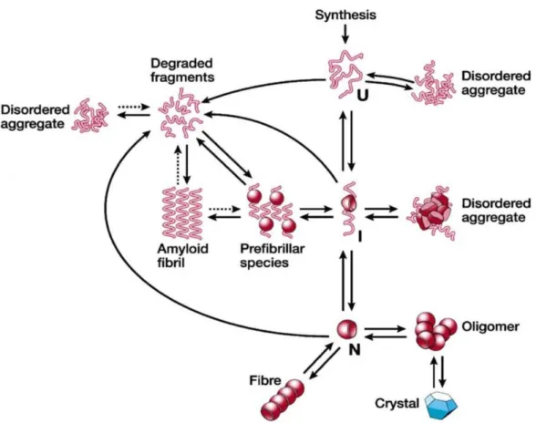
During the aggregation process, the polypeptide chains can adopt a lot of conformational states and interconvert among them on a wide range of time-scale (Figure 6). Amyloid nucleation is a complicated process due to the competition of the factors involved. In particular, it was shown that globular proteins need at least partial unfolding to be able to aggregate and form amyloid fibrils 37_{. In} some cases the presence of structured oligomers 38 or unstructured aggregates 39 has been reported as fibrils precursors. Aggregation pathway consist of a nucleation-dependent process and the results is the accumulation of rich in β-sheet fibrillar aggregates. To date, it is unclear whether aggregation proceeds via linear addition of single molecules or whether there are oligomeric intermediates, but the structural conversion to β-sheet results in the formation of prefibrillar intermediates. Protofibril assembly is followed by fibril formation, resulting in the characteristic inclusions observed in the amyloid-like diseases. Protofilaments and fibrils represent the last step of protein misfolding. The process is irreversible at this step since that mature fibrils structure is stable. Insoluble aggregates, as well as soluble oligomers, are characterized by the exposition of the hydrophobic core of the partially

(36)

36

unfolded protein, which attests the tendency of the protein to self-aggregate. The aggregation is prevented if protein concentration is below its critical threshold, while, if concentration is higher than critical threshold, a lag time exists before protein polymerization in order to favor nuclei formation. The presence of the stable fibrillar deposits in the organs of patients suffering from protein deposition diseases led initially to the reasonable postulate that amyloid fibrils were the main cause of the diseases. However, recent findings have raised the possibility that precursors to amyloid fibrils, such as low molecular weight oligomers and/or structured protofibrils, are the real pathogenic species, at least in neuropathic diseases 40,41.

Figure 6. Some of the many conformational states adopted by polypeptide chains. The transition from beta-structured aggregates to amyloid fibrils can occur by addition of either monomers or protofibrils (depending on the protein) to preformed beta-aggregates.

2.5 Spinocerebellar Ataxia Type-1 and AXH domain

Several neurological disorders arise from the previously explained protein aggregation and amyloid formation mechanisms. In case of polyglutamine (polyQ) diseases, the neurodegenerative disorders are caused by an unstable expansion of genomic cytosine-adenine-guanine (CAG) trinucleotide repeats beyond a specific threshold. In the healthy population, the number of CAG repeats lies between 10 to 51, while 55-87 CAG repeats is associated with the disease 42. The CAG tracts are translated into expanded glutamine regions in the respective proteins, promoting their self-assembly and amyloid structure formation. A large amount of experimental evidence has indicated a correlation between poly-Q containing inclusions and disease progression 43.

(37)

37

Within this context, Spinocerebellar ataxia type 1 (SCA1) is an inherited neurodegenerative disease belonging to the class of polyglutamine (polyQ) diseases. In fact, it is well established that SCA1 is mainly caused by polyQ expansion in Ataxin-1 (Figure 7a), a nuclear protein constituted by 820 residues 44. Despite the well-established correlation between polyQ expansion and disease onset and severity 45, other findings have demonstrated the importance of the AXH domain (Figure 7b) of Ataxin-1 in both modulating the development of the disease and influencing the aggregation process 46–49.

Figure 7. a) Ataxin-1 primary amino acid sequence. The structured AXH domain is also represented. b) Visual inspection of the AXH monomer. The N-terminal tail is highlighted in red.

It was reported that the isolated AXH has the tendency to misfold and aggregate into fibers without any destabilizing factor, such as temperature increase or chemical denaturants 48. Moreover, recent findings have shown that Ataxin-1 aggregation is strongly reduced by replacement of AXH domain with the homologous sequence of the transcription factor HBP1 48, confirming the important role of AXH in modulating the aggregation mechanism. Despite the importance of the AXH domain of Ataxin-1 in driving the Ataxin-1 aggregation process 46–49, the AXH self-association mechanism, is not yet clarified and several crucial questions remain open. The present PhD work employs enhanced sampling techniques to fully characterized the AXH aggregation pathway from monomer to tetramer, identifying several protein mutations responsible for the destabilization of the monomer/dimer/tetramer equilibrium (Chapter 3).

2.6 Alzheimer’s Disease and Amyloid Hypothesis

Among several theories proposed to explain the cause of Alzheimer’s Disease (AD), the amyloid hypothesis represents one of the most likely scenarios 50,51. More in detail, the amyloid hypothesis is based on the idea that a mutation on an amyloid precursor protein (APP) induces the aggregation of Aβ peptides, whose deposition into senile plaques is followed by the formation of neurofibrillary tangles and neuronal cell death 51. However, it is still not clarified if the formation of these fibrils is the cause or a secondary effect of the disease 52_{. The major components of AD-associated amyloid}

(38)

38

plaques are Aβ1–40 peptides but also the more toxic Aβ1–42 species 53, characterized by two additional amino acids and generated through a sequential cleavage of the amyloid precursor protein (APP) by β and γ secretases 54_{. In general, these peptides are able to oligomerize and then the resulting oligomers} can further aggregate giving rise to ordered fibrils and fibers 55. Several experimental studies have been focused on the molecular characterization of amyloid fibrils, given the intimate relationship between molecular structure and disease onset and severity 56.

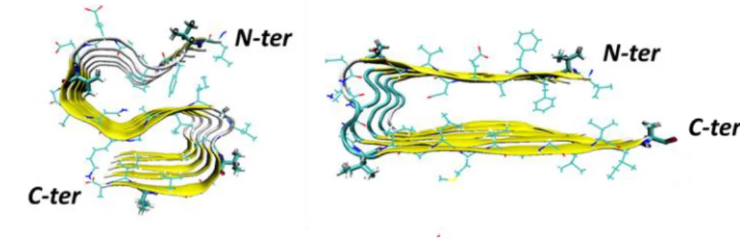
At present, all the Aβ1–40 species resolved by NMR, share a U-shaped motif, where the peptide chains form two β-strands connected by a loop region 57–61_{. In case of more toxic Aβ}

1–42 species, despite earlier NMR models exhibited the same U-shaped motif 58, more recent investigations demonstrated the possibility of S-shaped arrangements 62–67, characterized by three β strands (Figure 8). Interestingly, the S-shaped arrangement is not stable in case of Aβ1–40 species 68. Within this framework, the higher toxicity of Aβ1–42 species compared to Aβ1–40 may be explained by their ability to form S-shaped assembly. Such a correlation could arise if the S-shaped model i) was characterized by a more stable molecular architecture per se, or ii) was able to assemble into structures that are not possible by considering the U-shaped Aβ chains, as recently suggested 68. The present PhD thesis provides a molecular level understanding of the interactions governing the structural arrangement in Aβ1–42 species (Chapter 4). Outcomes of the study suggest that the molecular architecture of the protein aggregates might play a pivotal role in formation and conformational stability of the resulting fibrils.

(39)

39

Chapter 3

AXH Aggregation Pathway: From Monomer to Tetramer

Ataxin-1 is the protein responsible for the Spinocerebellar ataxia type 1, an incurable neurodegenerative disease caused by polyglutamine expansion. The AXH domain of Ataxin-1 plays a pivotal role in the misfolding and aggregation pathway responsible for the pathology onset. The present work employs classical and enhanced sampling techniques to fully characterized the AXH aggregation pathway from monomer to tetramer, identifying several protein mutations responsible for the destabilization of the monomer/dimer/tetramer equilibrium.

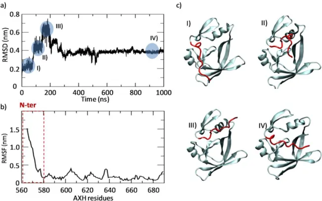
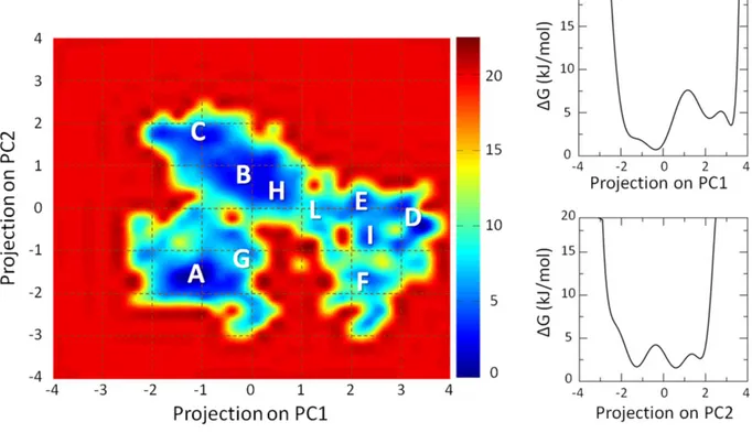
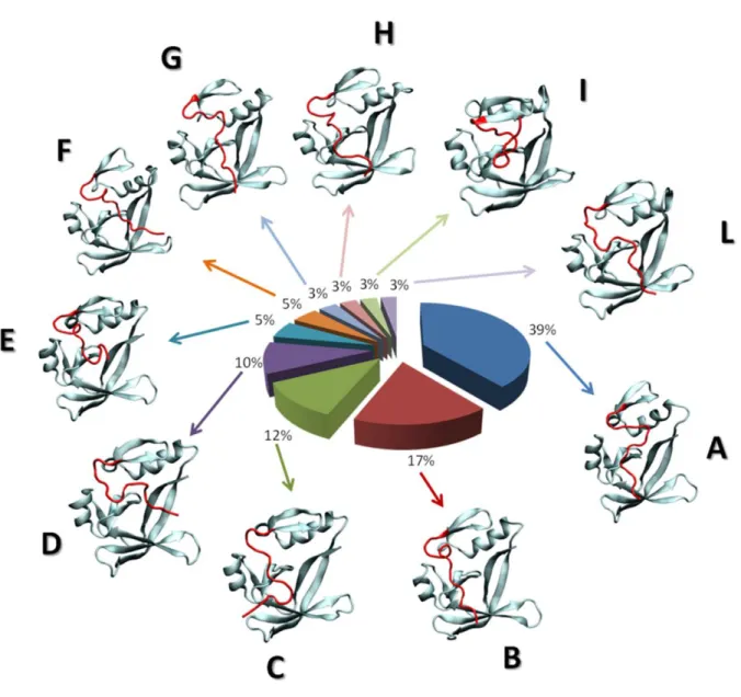
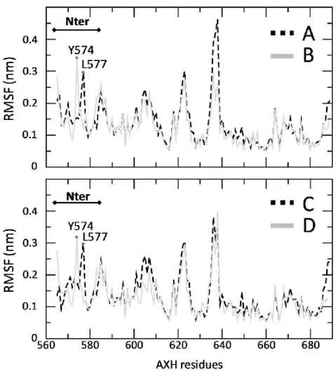
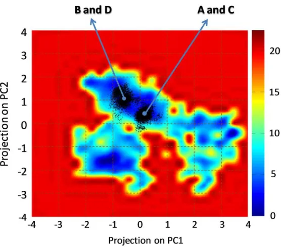
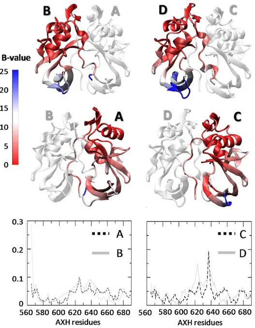
The Section 3.1 is focused on the description of the AXH monomer, revealing its substantial conformational fluctuations in physiological environment, especially in the N-terminal region. These fluctuations can be generated by thermal noise since the free energy barriers between conformations are small enough for thermally-stimulated transitions.

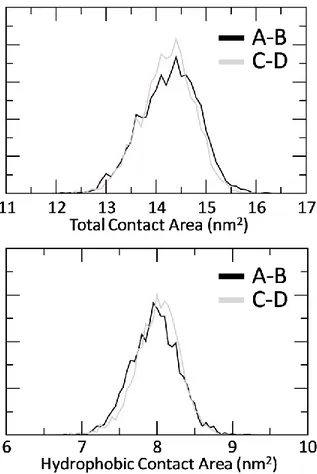
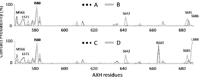
The Section 3.2 is devoted to the characterization of the AXH inter-monomer interface and the molecular description of the AXH monomer-monomer interaction mode. The computational results support previous experimental findings suggesting that interactions leading to the dimer formation can stabilize the N-terminal region of the AXH. Moreover, the importance of the I580 residue in mediating the AXH monomer-monomer interaction dynamics was fully explained with atomic resolution.

The Section 3.3 reports a computational study to identify the structural and energetic basis of AXH tetramer stability. Results of the study point the attention, for the first time, on R638 protein residue, which shown to play a key role in AXH tetramer stability. Therefore, R638 might be also implicated in AXH oligomerization pathway and stands out as a target for future experimental studies focused on self-association mechanisms and fibril formation of full-length ATX1.

(i) G. Grasso, M.A. Deriu, J.A. Tuszynski, D. Gallo, U. Morbiducci, A. Danani, Conformational fluctuations of the AXH

monomer of Ataxin-1, Proteins Struct. Funct. Bioinforma. 84 (2016) 52–59. doi:10.1002/prot.24954.

(ii) M.A. Deriu, G. Grasso, J.A. Tuszynski, D. Massai, D. Gallo, U. Morbiducci, A. Danani, Characterization of the AXH domain of Ataxin-1 using enhanced sampling and functional mode analysis, Proteins Struct. Funct. Bioinforma. 84 (2016) 666–673. doi:10.1002/prot.25017.

(iii) G. Grasso, U. Morbiducci, D. Massai, J. Tuszynki, A. Danani, M. Deriu, Destabilizing the AXH Tetramer by Mutations: