Contraction and partial contraction : a study of synchronization in nonlinear networks

(1)

Contraction and Partial Contraction:

Synchronization in Nonlinear Networks

by

Wei Wang

B.S., Thermal Engineering (1994)

Tsinghua University

M.S., Thermal Engineering (1997)

MASSACHUSETTS INSTWE OF TECHNOLOGY

MAY 0 5 2005

LIBRARIES

Tsinghua University

Submitted to the Department of Mechanical Engineering

in partial fulfillment of the requirements for the degree of

Doctor of Philosophy in Mechanical Engineering

at the

MASSACHUSETTS INSTITUTE OF TECHNOLOGY

February 2005

©

Massachusetts Institute of Technology 2005. All rights reserved.

Author ...

...

Department of Mec anical Engineering

December 16, 2004

Certified by ... ...

...

Jean-Jacques E. Slotine

Professor of Mechanical Engineering and Information Sciences;

Professor of Brain and Cognitive Sciences

'/

~Thepsis

Supervisor

Accepted by... ...

Lallit Anand

Chairman, Department Committee on Graduate Students

a Study of

(2)

(3)

Contraction and Partial Contraction: a Study of

Synchronization in Nonlinear Networks

by

Wei Wang

Submitted to the Department of Mechanical Engineering on December 16, 2004, in partial fulfillment of the

requirements for the degree of

Doctor of Philosophy in Mechanical Engineering

Abstract

This thesis focuses on the study of collective dynamic behaviors, especially the spon-taneous synchronization behavior, of nonlinear networked systems. We derives a body of new results, based on contraction and partial contraction analysis. Contraction is a property regarding the convergence between two arbitrary system trajectories. A non-linear dynamic system is called contracting if initial conditions or temporary distur-bances are forgotten exponentially fast. Partial contraction, introduced in this thesis, is a straightforward but more general application of contraction. It extends contrac-tion analysis to include convergence to behaviors or to specific properties (such as equality of state components, or convergence to a manifold). Contraction and partial contraction provide powerful analysis tools to investigate the stability of large-scale complex systems. For diffusively coupled nonlinear systems, for instance, a general synchronization condition can be derived which connects synchronization rate to net-work structure explicitly. The results are applied to construct flocking or schooling models by extending to coupled networks with switching topology.

We further study the networked systems with different kinds of group leaders, one specifying global orientation (power leader), another holding target dynamics (knowledge leader). In a knowledge-based leader-followers network, the followers obtain dynamics information from the leader through adaptive learning.

We also study distributed networks with non-negligible time-delays by using sim-plified wave variables and other contraction-oriented analysis. Conditions for contrac-tion to be preserved regardless of the explicit values of the time-delays are derived. Synchronization behavior is shown to be robust if the protocol is linear.

Finally, we study the construction of spike-based neural network models, and the development of simple mechanisms for fast inhibition and de-synchronization.

Thesis Supervisor: Jean-Jacques E. Slotine

Title: Professor of Mechanical Engineering and Information Sciences; Professor of Brain and Cognitive Sciences

(4)

(5)

Acknowledgments

First, I wish to express my deepest gratitude to my advisor, Professor Jean-Jacques Slotine. Without his consistent support, guidance and patience, none of the results in this thesis could be done.

I would also like to thank other two faculty members in my thesis committee, Professor Michael Triantafyllou and Professor Rodolfo Rosales. I appreciate their professional advice on my thesis work. The discussions with them were very stimu-lating.

I thank all my friends and labmates, who make my life in MIT enjoyable and easy. Special thanks go to Martin Grepl, who gave me many helps in the beginning of my research, Tu Duc Nguyen, who visited MIT very shortly but will be my friend for ever.

Finally and most importantly, I would like to thank my family. My parents and my sister have supported me with their selfless love since I was born. My wife Minqi, who accompanied me through my whole study in MIT, has shared each piece of my happiness and sadness. This thesis is dedicated to her.

This work was supported in part by grants from the National Institutes of Health and the National Science Foundation.

(6)

(7)

97 ... .. 97 ... .. 97 ... .. 99 . . . 102 105 106 107 107 109 110 113 113 116 ... 116 119 10 Concluding Remarks 59 59 64 64 65 70 72 72 72 74 75 77 78 78 79 82 85 85 88 90 93 94 95 ... ... ... ... ... ... ... ... ... ... . . . . . . . . . . . . . . . . . . . . . . . . . . . . . . . . . . . . . . . . . . . . . . . . . . . . . . . . . . . . . . . . . . . . . . . . . . . . . . . . . . . . . . .

(9)

List of Figures

2-1 Illustration of equilibrium point and line attractor ... . 18

3-1 Two bidirectionally coupled Van der Pol oscillators synchronize .... 26

3-2 Two Smale's cells anti-synchronize through diffusion interactions. . . 28

3-3 Two Van der Pol oscillators die through interactions ... . 29

4-1 An n 4 network with different symmetric structures ... 33

4-2 Four coupled Van der Pol oscillators synchronize with (a) chain, (b) one-way-ring, (c) two-way-ring, (d) all-to-all structure ... 37

4-3 Comparison of a chain network and a ring . ... 47

4-4 Comparison of three different kinds of networks . ... 48

4-5 Fast inhibition with a single inhibitory link ... 50

4-6 A single inhibitory link destroys network synchrony . ... 50

5-1 Evolution of virtual displacement of a sample switching network ... . 54

5-2 Closer to the local agreement, closer to the global ... 57

6-1 Networked systems with (a). a power leader (the most left node); (b). a knowledge leader (the hollow node); (c). both leaders ... 59

6-2 Synchronization propagates in a network with non-uniform connectivity. 62 6-3 vi of the neurons in (a).the inner group, (b).the outer group with inter-group links ... . 63

6-4 vi of the neurons in (a).the inner group, (b).the outer group without inter-group links . . . 63

6-5 Simulation of Example 6.2.1. (a).States vi (i = 1,2) versus time; (b).estimator error versus time ... 66

6-6 Simulation of Example 6.2.2. (a).States v (i = 1, ... ,6) versus time; (b).estimation error a4 of one follower versus time ... 70

6-7 A solution trajectory of system (6.10) leaves and re-enters the region Q: vi <vo ... 73

7-1 Two interacting systems with delayed communications ... . 78

7-2 Two interacting systems with time-delayed diffusion couplings ... . 80

7-3 Simulation results of two coupled mass-spring-damper systems with (a) PD control and (b) D control. Parameters are b = 0.5, w2 ₌_5, Tl = 2s, T₂1 =4s, kd = 1, kp 5 in (a) and kp = 0 in (b). Initial conditions, chosen randomly, are identical for the two plots . ... 82

(10)

7-4 Simulation results of Example 7.1.2 with (a). T1 2 = T21 = 0 and with (b). T1 2 = 2s, T2 1 = 4s. The parameters are b = b2 = 0.5,

2 = 02 = 5, k1 2 = k2 = 0.2, and Fe = 10. Initial conditions, chosen randomly, are identical for the two plots. Convergence to a common equilibrium point independent to the time delays is achieved in both

cases ... 84

7-5 Simulation results of Example 7.2.1 without delays and with delays. Initial conditions, chosen randomly, are the same for each simulation. Group agreement is reached in both cases, although the agreement value is different ... 88 7-6 Simulation results of Example 7.2.2 without delays and with delays.

Initial conditions, chosen randomly, are the same for each simulation. In both cases, group agreement to the leader value x0 is reached. .... 90

7-7 Simulation results of Example 7.2.3 without delays and with delays. In both plots, the dashed curve is the state of the leader while the solid ones are the states of the followers, which converge to a periodic solution in both cases regardless of the initial conditions ... . 91 9-1 The FN model (9.1) in the state space. (a) Illustration of the

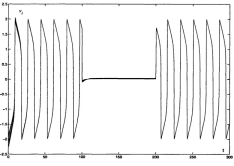
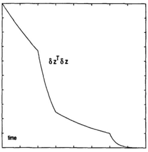
excitabil-ity feature; (b) illustration of the WTA computation ... ... . 106 9-2 Basic WTA network structure ... ... . 108 9-3 Simulation of WTA computation with n = 10. (a) States vi versus

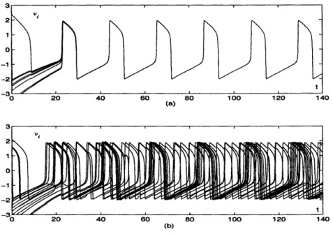
time (the dashed curve represents the state of the neuron receiving the largest input); (b) state z versus time ... . 108 9-4 A distributed WTA network structure ... . 111 9-5 Simulation of distributed WTA computation. (a) States vi versus time;

(b) inhibitions zi versus time ... 111

9-6 Simulation result of WTA computation with varying inputs. (a) States vi versus time; (b) inputs Ii versus time ... 112 9-7 Simulation result of WTA computation with multiple winners .... . 112 9-8 Simulation of k-WTA computation. (a) States vi versus time; (b)

inputs Ii versus time ... 115 9-9 Simulation of soft-WTA computation. (a) States vi versus time; (b)

global inhibition z versus time ... . 115 9-10 Simulation of fast coincidence detection. The upper plot shows

En=

max(0, vi)

(11)

Chapter 1 Introduction

The complexity of the world we live is based on accumulation and combination of simple elements. Collective behaviors of dynamic networked systems, such as spon-taneous synchronization, pervade nature at every scale. Although the study of these natural phenomena has lasted for a few centuries, it remains a mystery and attracts more and more attention from researchers working across disciplines. In this thesis, a body of new results on nonlinear networked systems is derived based on contraction and partial contraction analysis.

Contraction is a property regarding the convergence between two arbitrary sys-tem trajectories. A nonlinear dynamic syssys-tem is called contracting if initial condi-tions or temporary disturbances are forgotten exponentially fast. The basic results of Contraction Theory are briefly reviewed in Chapter 2, followed which we derive a sufficient condition to preserve contraction through an arbitrary feedback combi-nation, and([ then develop the theory of partial contraction. Partial contraction (or meta-contraction) is a straightforward but more general application of contraction. It extends contraction analysis to include convergence to behaviors or to specific prop-erties (sucl-h as equality of state components, or convergence to a manifold). Not surprisingly contraction can be considered as a particular case of partial contraction. The development of Partial Contraction Theory provides a general analysis tool to investigate the stability of large-scale complex systems. In particular, it is power-ful to study synchronization behavior by inheriting the central feature of contraction that, convergence and explicit dynamics are treated separately, leading to signifi-cant conceptual simplifications. We illustrate the idea in Chapter 3 by investigating the behaviors of two coupled oscillators. Chapter 4 generalizes the analysis to cou-pled networks with various structures and arbitrary sizes. For nonlinear systems with positive-definite diffusive couplings, we show that synchronization will always occur if coupling strengths are strong enough, and an explicit upper bound on the correspond-ing threshold can be computed through eigenvalue analysis. Rather than linearized, the results are exact and global, and can be easily extended to study nonlinear cou-plings, to unidirectional coucou-plings, and to positive semi-definite couplings as well. We further connect the synchronization rate to a network's geometric properties, such as connectivity, graph diameter or mean distance. A fast inhibition mechanism is also studied.

(12)

In fact, synchronization research has a very close connection with group cooper-ation study. Recently, there is considerable interest in understanding how various animal aggregations, such as bird flocks or fish schools, coordinate their collective motions to perform useful tasks. A great effort has made to achieve similar behaviors of artificial multi-agent systems, such as vehicles or satellites, with distributed cooper-ative control rules. In Chapter 5 we build corresponding flocking or schooling models by extending the previous analysis to coupled networks with switching topology.

We study the networked systems with different kinds of group leaders in Chapter 6. The leader specifying global orientation is named power leader, while that holding target dynamics is knowledge leader. In a knowledge-based leader-followers network, the followers obtain dynamics information from the leader through adaptive learning. Such a mechanism may exist in many natural processes, for instance, in evolutionary biology or in disease dynamics. Synchronization conditions for both kinds of networks are derived based on contraction or graph analysis.

In real-world engineering applications, communications between different systems always involve non-negligible time-delays. In Chapter 7, we conduct a contraction analysis on time-delayed feedback communications using simplified wave variables. A condition to preserve contraction regardless of the delay values is derived. The

approach is then applied to study the group cooperation problem with time-delayed communications.We show that synchronization is robust to time delays with linear protocol, no matter if the dynamics is continuous or discrete-time, or if the network is leaderless or leader-followers. A different but more general study of time-delayed

nonlinear systems will be presented in Chapter 8.

Finally, in Chapter 9 we develop an effective de-synchronization mechanism, based on which a networked system converges to a well-ordered phase-locking solution very quickly, and thus allows us to construct neural network models with the ability to perform fast spike-based computations, such as coincidence detection and winner-take-all. These basic computational units are able to be accumulated to execute higher-level brain functions, the implementation of which will facilitate the realization of, for instance, binding in machine vision and perception.

(13)

Chapter 2 Contraction and Partial

Contraction

Basically, a nonlinear time-varying dynamic system will be called contracting if initial conditions or temporary disturbances are forgotten exponentially fast, i.e., if trajec-tories of the perturbed system return to their nominal behavior with an exponential convergence rate. The concept of partial contraction allows to extend the applications of contraction analysis to include convergence to behaviors or to specific properties (such as equality of state components, or convergence to a manifold) rather than trajectories.

2.1 Contraction Theory

Contraction Theory is a new nonlinear analysis tool, which investigates the stability with respect to trajectories. Here we briefly summarize its basic definitions and main results, details of which can be found in [81, 82].

Consider a nonlinear system

k= f(x,t) (2.1)

where x E R X1 is a state vector and f is an m x 1 vector function. Assuming f(x, t) is continuously differentiable, we have

dt_(xTax) ₌ _{2 6xTAx}₌_{2 3xT} _x_K₂_Amax _6xTOx

where x is a virtual displacement between two neighboring solution trajectories, and Ama(x, t) is the largest eigenvalue of the symmetric part of the Jacobian J = f. Hence, if Amax(x,t) is uniformly strictly negative, any infinitesimal length

116x1

converges exponentially to zero. By path integration at fixed time, this implies in turn that all the solutions of the system (2.1) converge exponentially to a single trajectory, independently of the initial conditions.

More generally, consider a coordinate transformation

(14)

where E(x, t) is a uniformly invertible square matrix. One has

d (6zT z) = 2 SZT6Z = 2 ZT ( + M)e - 1

so that exponential convergence of J]z1] to zero is guaranteed if the generalized

Jaco-bian matrix

F ( + 8 1f )e-1 (2.3)

is uniformly negative definite. Again, this implies in turn that all the solutions of the original system (2.1) converge exponentially to a single trajectory, independently of the initial conditions.

By convention, the system (2.1) is called contracting, f(x, t) is called a contracting

function, and the absolute value of the largest eigenvalue of the symmetric part of F

is called the system's contraction rate with respect to the uniformly positive definite

metric M = eTe.

Note that in a globally contracting autonomous system, all trajectories converge exponentially to a unique equilibrium point [81, 133].

2.2 Feedback Combination of Contracting Systems

One of the main features of contraction is that it is automatically preserved through a variety of system combination. Consider two contracting systems and an arbitrary feedback connection between them. The overall virtual dynamics can be written as

d Jzl Fzz1l

dt

[Z2 F Z2

with the symmetric part of the generalized Jacobian in the form

Fs= 2 (F + FT)= GT _F

(the subscript symbol s represents the symmetric part of the matrix). By hypothesis the matrices Fla and F28are uniformly negative definite. Then F is uniformly negative

definite if and only if ([51], page 472)

F2 < GT F G

Thus, a sufficient condition for the overall system to be contracting is that

A(F18) A(F2s) > 2(G) uniformly Vt 0 (2.4)

where A(Fia) is the contraction rate of Fi, and a(G) is the largest singular value of

G. Indeed, condition (2.4) is equivalent to

(15)

and, for an arbitrary nonzero vector v,

vT F2s v < Amax(F2s) v v

< Amjn(F 1 ) 2 (G) vTv

< Amin(Fj1) vTGTGv < vT GT F1 G v A simple example was studied in [81] where

F = ,

-G T F2

The result (2.4) can be applied recursively to larger combinations. Note that, from the eigenvalue interlacing theorem [51],

A(F,) < min A(Fis)

2.3 Partial Contraction Theory

The concept of partial contraction came out firstly when we worked on the study of network synchronization, since which its unique capacity and flexibility have been proved in more and more application fields.

Theorem 2.1 Consider a nonlinear system of the form

x:k = f(x,x,t)

and assume that its auxiliary system

y = f(y, x(t), t)

is contracting with respect to y. If a particular solution of the auxiliary y-system verifies a smooth specific property, then all trajectories of the original x-system verify this property exponentially. The original system is said to be partially contracting.

Proof: The virtual, observer-like y-system has two particular solutions, namely y(t) = x(t) for all t > 0 and the solution with the specific property. For a con-tracting system, all solutions converge together exponentially regardless of the initial conditions. This implies that x(t) verifies the specific property exponentially. E

Note that contraction may be trivially regarded as a particular case of partial contraction. Consider for instance an original system in the form

(16)

where function c is contracting in a constant metric. The auxiliary contracting system may then be constructed as

y = c(y,t) + d(x(t),t)

In this example, contraction is a particular case of partial contraction when d = 0. If d

$

0, the specific property of interest may consist e.g. of an equilibrium point, or a relationship between state variables which we will illustrate through the following sections. Here we study a few simple examples.

Example 2.3.1: Consider the system taken from [60]

[±X] ] [ -1 X1 ][ X1]

X2 -1 x 2

to which we construct an auxiliary system

Y2 -xl -1 Y2

The y-system is contracting and has two particular solutions [Y ] = [i

]

and

Y2 x2

[Y2 ] = [0] Thus, according to Partial Contraction Theory, xl and x2 will both

tend to 0 exponentially. 0

Example 2.3.2: Consider the system from [131]

{

xl = 2 - x ( 4

+

2x2 - 10)

x2 = - - 3x5 (x4 + 2x2 - 10)

which is equivalent to

d

4 X2_10) -

)6 (4+

-10)

( 1 + 2x2 - ) = -(4x 4x1 0 + 12x ) (4 + 2x2 - 10) and has an auxiliary system

= - (4x0l° + 122

)

y

The y-system has two particular solutions y = x4+ 2x2-10 and y = 0, and is contracting as long as not both xi(t) and x2(t) equal to 0. It is then easy to show that, the system stays at the origin if xl(0) = x2(0) = 0. Otherwise it tends to reach

x (t)4 + 2 x2(t)2 = 10

exponentially. 0

Example 2.3.3: Consider a convex combination or interpolation between contracting dynamics

(17)

where the individual systems = fi(x,t) are contracting in a common metric M(x) =

0T(x)3(x) and have a common trajectory xo(t) (for instance an equilibrium), with all cai(x, t) > 0 and Ei j &(x, t) = 1. Then all trajectories of the system globally exponentially converge tIo the trajectory xo(t). Indeed, the auxiliary system

2/= E cei (x, t) fi (Y t)

is contracting (with metric M(y) ) and has x(t) and xo(t) as particular solutions. 0 The notion of building a virtual contracting system to prove exponential conver-gence applies also to control problems[60, 135]. Consider for instance a nonlinear system of the form

x = f(x,x,u,t)

and assume that the control input u(x, Xd, t) can be chosen such that

Xd = f(xd, x, u, t)

where xd(t) is the desired state. Construct now the auxiliary system

y = f(y,x,u,t)

If the y-system is contracting, then x tends xd exponentially. Example 2.3.4: Consider a rigid robot model

H(q)i + C(q, ) + g(q) = r and the energy-based controller [131]

H(q) ir + C(q, q)qr + g(q) - K(q - qr) =

with K a constant symmetric positive-definite matrix. The virtual y-system H(q) + C(q, )y + g(q) - K( - y) =

has 4 and r as two particular solutions, and furthermore is contracting, since the skew-symmetry of the matrix H - 2C implies

d

dt &YTH6Y =-25yT(C + K)6y + 5yTI2jy =-25yTK6y

Thus

4 tends to

4r exponentially. Making then the usual choice r = id - A(q - qd)

creates a hierarchy and implies in turn that q tends to qd exponentially. O

2.4 Line-Attractor

Recent research in computational neuroscience points out the importance of contin-uous attractors [127, 71]. If a system contains a global stable equilibrium point, all

(18)

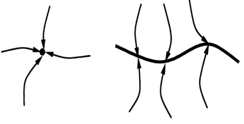
solutions converge to this point attractor regardless of initial conditions. If a system contains a line attractor, all solutions will converge to this line, and the resting point on this line depends on initial conditions. Figure 2-1 illustrates the difference between these two types of attractors. In this section, we use partial contraction theory to study line attractor.

Figure 2-1: Illustration of equilibrium point and line attractor.

2.4.1 Line-Attractor

Consider [47] a nonlinear neural network model

T'i + xi = [ wji xj + bi ]+ i= ,...,n

with [a]+ = max(O, a) and constant r > 0, or in matrix form

Tx + x = [Wx + b]+

with WT = W = [wj]. If I- W is positive semi-definite and b is in its range space, a line attractor exists [47]. To prove global exponential stability of this line attractor, arrange the eigenvalues Ai of I- W in increasing order, with 2 > A1 = 0.

The corresponding eigenvectors uj represent an orthonormal basis of the state space. Consider now the auxiliary system

T- + = [Wy + b]+ + 2 UluT(x(t)-Y) (2.5)

Note that given positive initial conditions, all components of x and y remain posi-tive. To apply partial contraction analysis, we need to do two things: first prove the auxiliary system is contracting, and then find a specific property for y.

contraction proof.

To prove the auxiliary system (2.5) is contracting, we use contraction analysis re-sults for continuously switching systems [82, 84]. Consider an arbitrary number of

(19)

continuously differentiable flow fields

x = f (x, t)

which are all contracting with respect to the same continuous (x, t). Now switch

arbitrarily among these different flow fields f. If the resulting flow is continuous in x for any time t > 0, the overall system is contracting. A detailed proof for system (2.5) to be contracting can be found in Appendix. The overall contraction rate is lower bounded by _2r''.

specific property:

Besides y = x(t), there exists another particular solution for the auxiliary system (2.5) which is

y = e + yoo Ul

Here e is a constant vector satisfying (I- W) e = b and y is a scalar variable defined by

Ty + A2Y = A2 U (x-e)

Note that we used uTu = 1 and the fact that, given positive initial conditions, one has

[Wy+b]+ = [y+b-(I-W )(e+y ,ul)]+=[y]+ = y

Thus, according to partial contraction theory, x(t) verifies exponentially the spe-cific property that (x(t) -e) is aligned with ul. Hence all solutions of the original system converge exponentially to a line attractor of the form

x = e + xO, Ul

where xOo = 0 using the original x dynamics. The actual value of xoo is determined by the initial conditions.

2.4.2 Generalized Line-Attractor

In this section, we study a generalized non-switching line-attractor model. Consider a nonlinear system

x = f(x, t)

with Jacobian J(x,t) = of We assume J(x,t) that is symmetric, and arrange its eigenvalues Ai = Ai(x, t) i = 1,..., n in increasing order. The corresponding eigen-vectors u/ = ui(x, t) represent an orthonormal basis of the state space.

Theorem 2.2 For the general nonlinear model described above, if V i = 2,. .. , n, Ai <

0, A1 is upper bounded, and ul is constant, then all solutions of the original system

will converge to an attractor of the form

(20)

where x~ (t) may depend on initial conditions. The convergence rate is lower bounded by 1A21.

Proof: The virtual dynamics of the original system is

6* = J(x,t) x (2.7)

Consider an auxiliary virtual dynamics of the form

y = J(x,t) 3y + ko(X,t) ulu (y - x) (2.8) and choose k(x, t) = A2(x, t) -Al (x, t). Then this auxiliary dynamics is contracting,

since

n

J(x,t) + ko(X,t) uluT = ZAi ,uiuT+ k uu < 2(x,t) I

Next, a particular solution of the auxiliary system (2.8) is Jy = ulby¢, where

= (A + k) y - k uT x = A2 hy - ( 2 - )uT 6x

Thus, from partial contraction, Sx converges exponentially to the form 6x = ul,6x, where, by replacing in (2.7),

5o= Al 6x X

Hence all solutions x(t) of the original system exponentially satisfy (2.6), where e(t) depends on the explicit form of f. Note that if Al > 0, the dynamics on the line

attractor is unstable. 0

2.5 Appendix: Contraction Analysis of (2.5)

To prove that the system (2.5) is contracting, we assume V i, j, wij > O. This implies that all couplings are excitatory. Such a matrix W = [wij] is named a nonnegative

matrix [51].

Lemma 2.1 If W is nonnegative and I - W is positive semi-definite, then I + W,

and all their principle submatrices are positive semi-definite.

Proof:

Since Ai(I- W) = 1 - Ai(W), we have

V i = 1,...,n Ai(W) < 1 with Amx(W) = 1

According to extended Perron's Theorem [51](page 503), if W is nonnegative, then its spectral radius p(W) is an eigenvalue of W, which implies that p(W) = 1 in this case. Thus A(I + W) = 1 + Ai(W) > 0, i.e., I + W is positive semi-definite. Furthermore, all submatrices of I - W and I + W are positive semi-definite, which

(21)

To conduct contraction analysis for system (2.5), we first study the case when Vi = 1,.. . n, [ i wji yj + bi + > 0. Thus the system's dynamics is actually

r

+ y

=

Wy + b + A2 U1UT (X(t)-y)

which is contracting since Vv ~ 0, v = Ein1 kitu, and

= vT(I - W)v + A₂ vTulUTv

n

= E(kui)T(I- W)(kiui) + A2(kui)TuuT(kui)

i=2 n

=

i=2 Aik2 + A₂kl2 > Moreover, Amin(I- W + 2 ululf) mvT(I- W + A2 luT)v

=

mm vTv#0 vTv

E-n_-=

Si=2 Ak, + Ak +A2 > A%2

=

n k2 > A

i=l i

Next, by assuming W = [wij] = and setting vT = [v_ 1 v], one has

vT(I - W + A₂ uluT)v = VT([ I-Wn_ _T 1 -Wn Wn--1n T wT Wn ] with wn = [ln ... W(n-l)nT + n2 uu)v

+

2 ulu[v

Thus, if for element n(or any other one) [ En win yj + bn ]+ = 0, the Jacobian of (2.5) changes to F =-(I-

[

-1 Wn ]+ A2 UlUT), which is still contracting since

0 0 + 2U1Twihi tl otatn ic - VTFV = VT([ I -Wn_ 1 I T n 1Wn ₊ A₂ UlUT) V

-lwn

= vT(I W + A2 UlUT)v + vT( [I -Wn > vT( I -w+A 2 uu l )v > 0 1 + Wnn + A2 UlUlT)v 1A2vTv 2 vT(I - W + A₂ ulUlT)v - Vn(I- Wn-1 )vn-1 + vT(1 - Wnn)Vn -2Vn(V¥lWn) > 2vTv + A₂vTuu V -Wn - Wnn

(22)

The analysis can be easily extended. For instance, one can assume W

= [ij] =

[

Wn-2 T Wn-1 -T W_n Wn-1 W(n-1)(n-1) W(n-l)n Wn Wn(n-1) Wnn

If for both elements n - 1 and n [ Ei wji yj + bi ]+ - 0, the Jacobian is

+ A2 lulT)

which is contracting since

-vTFv = lvT(I W + A2uluT)V +

0 .

I + W nW(n-)(n-1) Wn(n-W(n-l)n nn + A2 u uT)v > lA 2v v 2

We conclude that, system (2.5) as a continuous switching system is contracting because each of its piece-wise system is contracting based on an identity metric. Furthermore, the overall system's contracting rate is lower bounded by A._27''

T(

[-

W-2

2

0

Wn-2 Wn-l Wn

F = -(I - 0 0 0

(23)

-Chapter 3

Two Coupled Oscillators

Initiated by Huygens in the 17th century, the study of coupled oscillators involves today a variety of research fields, such as mathematics [24, 120, 141, 142], biology [21, 99, 140], neuroscience [14, 50, 67, 89, 101, 130, 177, 182], robotics [10, 53, 64, 68], and electronics [20], to cite just a few. Theoretical analysis of coupled oscillators can be performed either in the phase-space, as e.g. in the classical Kuramoto model [69, 142, 175], or in the state-space, as e.g. in the fast threshold modulation model [66, 137, 138]. While nonlinear state-space models are much closer to physical reality, there still does not exist a general and explicit analysis tool to study them. Starting from this chapter, we develop a new method based on partial contraction theory.

The analysis is carried out in two steps. First, we prove that the whole coupled system is contracting or partially contracting, implying for instance that all subsys-tems converge together regardless of the initial conditions. In a second, easy step, the final behavior is determined. We illustrate the idea in this chapter by investigating the coupled networks composed by two oscillators. The theoretical results are then simulated with general Van der Pol oscillators [99, 141], whose relaxation behavior can be made to resemble closely some standard neuron models. In contrast with pre-vious approaches such as e.g., [17, 119, 139], our results are exact and global. In fact, the analysis method we developed is not limited by individual systems' dynamics. It can also be applied to study any other coupled systems rather than oscillators.

3.1 One-Way Coupling Configuration

Consider a pair of one-way (unidirectional) coupled identical oscillators

{

l- f(xi,t)

k2 =f(x2, t) + u(x)-u(x 2) (3.1)

where x, 2 E Rm are the state vectors, f(xi,t) the dynamics of the uncoupled oscillators, and u(xl) - u(x2) the coupling force.

Theorem 3.1 If the function f - u is contracting in (3.1), two systems xl and x2

(24)

Proof: The second subsystem, with u(xl) as input, is contracting, and x2(t) = x1(t)

is particular solution. 0

Example 3.1.1: Consider two coupled identical Van der Pol oscillators

1 + (x2- 1)±l + W2X1 = 0

X2 + a(X2 - 1)±2 + w2x2 = aC(Xl - 2)

where a, w and n ae strictly positive constants (this assumption holds for all the Van der Pol examples). Since the system

-+ a(x2 ₊_K_- ₁₎₅₊_w2_x₌_u(t)

is semi-contracting for n > 1 (see Appendix 3.3), x2 will synchronize to Xl asymptotically.

0

Note that a typical engineering application with an one-way coupling configuration is observer design, in which case xl represents the plant state needed to be measured. The result of Theorem 3.1 can be easily extended to a network containing n oscillators with a chain structure (or more generally, a tree structure)

x*1 = f(xl,t)

X2 = f(x2, t) + u(xl) - u(x2) (3.2)

I. . .

xn f(Xn, t) + u(xnl 1) - (xn)

where the synchronization condition is the same as that for system (3.1).

3.2 Two-Way Coupling Configuration

The meaning of synchronization may vary in different contexts. In this thesis, we de-fine synchronization of two (or more) oscillators xl, x2 as corresponding to a complete

match, i.e., xl = x2. Similarly, we define anti-synchronization as xl = -x2. These

two behaviors are called in-phase synchronization and anti-phase synchronization in many communities.

3.2.1 Synchronization

Theorem 3.2 Consider two coupled systems. If the dynamics equations verify

x -h(x1, t) = x2 -h(x 2, t)

where the function h is contracting, then xl and x2 will converge to each other

(25)

Proof: Given initial conditions x1(0) and x2(0), denote by xl (t) and x2(t) the

solu-tions of the two coupled systems. Define

g(x1, x2, t) = i - h(xi, t) = x2 - h(x2, t)

and construct the auxiliary system

y = h(y, t) + g(x1(t), x2(t), t)

This system is contracting since the function h is contracting, and therefore all solu-tions of y converge together exponentially. Since y = x1(t) and y = x2(t) are two

particular solutions, this implies that x1(t) and x2(t) converge together exponentially. 0

A few remarks on Theorem 3.2:

* Theorem 3.2 can also be proved by construct another auxiliary system S Y= h(yi,t) + g(x1,x2,t)

y2

=

h(y

2

,t) +

g(x

1

,x

2

,t)

which has a particular solution verifying the specific property Yl = Y2. In fact, this auxiliary system is composed of two independent subsystems driven by the same inputs. Thus, the proof can be simplified by reduce the dimension of the y-system.

* Theorem 3.1 is a particular case of Theorem 3.2. So is, for instance, a system of two-way coupled identical oscillators of the form

I X1 = f(xi,t) + u(x2)-u(x1)

I 2 = f(x2,t) + (xl)-U(X2)

In such a system xl tends to x2 exponentially if f - 2u is contracting.

Further-more, because the coupling forces vanish exponentially, both oscillators tend to their original limit cycle behavior, but with a common phase.

* Although contraction properties are central to the analysis, the overall system itself in general is not contracting, and the common phase of the steady states is determined by the initial conditions x1(0) and x2(0). This point indicates

the difference between contraction and partial contraction.

* The result of Theorem 3.2 can be easily extended to coupled discrete-time tems, using discrete versions [81] of contraction analysis, to coupled hybrid sys-tems, and to coupled systems expressed by partial-differential-equations(PDE).

Example 3.2.1: Consider again two coupled identical Van der Pol oscillators

+ (X-l) + w2xl = aK₁(i 2-l X2 + a(x -1)d₂ + W2x2 = 2(l - 2)

(26)

One has

X1 + a(X2 + --1 + 2 - 1)Xil + W2X1 = X2 + a(X2 + K1 + 2 - 1)12 + W2X2

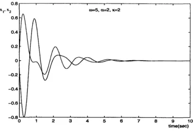
According to Theorem 3.2 and the result in Appendix 3.3, we know that these two oscillators will reach synchrony asymptotically if

E1 + E2 > 1

for non-zero initial conditions. Figure 3-1 shows a tions are chosen randomly.

x1. x2

simulation result, where initial condi-J

timre(sec)

Figure 3-1: Two bidirectionally coupled Van der Pol oscillators synchronize.

3.2.2 Anti-Synchronization

In a seminal paper [136] inspired by Turing's work [99, 153], Smale describes a mathe-matical model where two identical biological cells, inert by themselves, can be excited into oscillations through diffusion interaction across their membranes. Using Theo-rem 3.2, we can build a coupled system

{

x₁

=

h(x1 , t) + u(x2, t)-u(x1, t)

|2 = h(x2, t) + (x1, t) - U(X₂, t)

(3.4) to describe Smale's model.

Theorem 3.3 If the uncoupled dynamics h in (3.4) is contracting and odd in x, x +

x2 will converge to zero exponentially regardless of the initial conditions. Moreover, for non-zero initial conditions, x1 and x2 will oscillate and reach anti-synchrony if the system

(27)

has a stable limit-cycle.

Proof: Theorem 3.3 can be proved by change the sign of x2 in Theorem 3.2, or by construct an auxiliary system

Yj = h(yl,t) + g(xl,x2, t) Y'2 = h(y2,t) - g(xl,x2, t)

with g(x1, x2, t) = u(x2, t)- u(x1, t). The y-system has a particular solution verifying the specific property yl = -Y2.

Example 3.2.2: Consider specifically Smale's example [136], where

h(x,t) = A X2 +

[

]

u(x) = K x2 x3 0

2

Kx3 LX4 0 X4 with

[

1+a 1 ya 0 ya A -1 a 0 ya K- 0 a 0 -ya

-'ya 0 2a 0 -7a 0 -2a 0

L0 -Sya 0 2a 0 -- ya 0 -2a

For a < -1, h has a negative definite Jacobian and thus is contracting, and h-2u yields a stable limit-cycle, so that the two originally stable cells are excited into oscillations for non-zero initial conditions. Requiring in addition that XV < -y < 3/2 guarantees that all the eigenvalues of K are real and strictly positive, so that K can be transformed into a diagonal diffusion matrix through a linear change of coordinates. 0 Example 3.2.3: Smale's example can be simplified by directly using two damped Van der Pol oscillators

{

x + a(x2+ 2, - 1)±1 + w2xl = -(2 - xl) X2 + a(x 2 + 2K - 1)42 + w2x2 = -an(xi - 2)

with the simulation result plotted in Figure 3-2.

0

3.2.3 Oscillator-Death

Inverse to Smale's effect, there is a phenomenon called oscillator-death (or amplitude-death) [5, 8, 121] where oscillators stop oscillating and stabilize at constant steady states after they are coupled.

Theorem 3.4 Oscillator-death happens if the dynamics of the whole coupled network

(28)

x_i,

Figure 3-2: Two Smale's cells anti-synchronize through diffusion interactions.

Example 3.2.4: Couple two Van der Pol oscillators with asymmetric forces

{

1 + ac(x2 - 1).l + W2X1 = an(.2 - 1)

X2 + a(X 2 - 1)2 + W2X2 = Cf(-Xl - X2)

(3.5) where v > 1. By introducing new variables Yi and Y2 as that in system (3.8), we get a generalized Jacobian -a(X 2+ - 1) w am -w 0 0 -an 0 -a(x 2+n-1) 0 0 0 01 WI 0] <0

whose symmetric part is simply that of two uncoupled damped Van der Pol oscillators.

Thus both systems will tend to zero asymptotically. 0

3.2.4 Coupled Van der Pol Oscillators - a general study

As a conclusion of this section, we now consider two identical Van der Pol oscillators coupled in a very general way:

IX1 + a(X2 I2 + (x2

- 1)il +W 2X₁ = C (Y2 -i Xl)

- 1)52 + 2x2 = a (i -- 52)

(3.6)

where a is a positive constant. It can be proved that, as long as the condition I I > 1

(29)

XI,

time(sec)

Figure 3-3: Two Van der Pol oscillators die through interactions.

is satisfied, x converges to x2 asymptotically for all 7y > 0 while x converges to

-x 2 asymptotically for all y < 0. Note that if -y = 0 we get two independent

stable subsystems. Both x and x2 tend to the origin, which can be considered as a

continuous connection between > 0 and y < 0. This result agrees with the common intuition that excitatory coupling leads to synchrony while inhibitory coupling to anti-synchrony.

Next we need to study the stable behavior of the coupled systems in order to make sure that if they keep oscillating or tend to a stationary equilibrium. Assume first that y > 0, we have

xi a c(2-)i - 2xi -- ( - _{) ti} i = 1,2

which gives the stable dynamics of x1 and x2 as

Xi + a(x + - 1)>i + 2xi = O.

This dynamic equation has a stable limit cycle if y > - 1 or a stable equilibrium point at origin otherwise. A similar result can be derived for -y < 0, where xl and x2

reach anti-synchrony if y < 1 - n or tend to zero otherwise. Also note that:

* Setting = 1, xl and x2will keep oscillating for all y ~ 0. Oscillator-death as a

transition state between synchronized and anti-synchronized solutions does not exist except when -y = 0.

* In general, a positive value of -y represents a force to drive synchrony while a negative value to drive anti-synchrony. Hence it is easy to understand the behavior of system (3.5) where the coupling to the first oscillator tries to

(30)

syn-chronize but the coupling to the second tries to anti-synsyn-chronize, with equal strength. A neutral result is thus obtained. In fact, if we look at a coupled system with non-symmetric couplings

I

X + a(x -1) + w2x₁ = a (1l2 - J)

{

+ (x2 - 1) 2 + wx 2 = a (2i 1 - K2X2)

the condition for oscillator-death is

hi>1, 1K2>1 , (-1 )(2-1)> (71Y + 2) /4.

* If we add extra diffusion coupling associated to the states x and x2 to

sys-tem (3.6)

{

+ a(x2 - 1)l₁ + w2x1 = a (Y2 - K) + a (X ₂- Rx) /X2 + a(x - 1) 2 + w2x₂ = a (7- x₂) + a Xl-x)

where n and are both positive, the main result preserves as long as y7 > 0. If the condition I y I > 1 - n is satisfied, xl converges to x2 asymptotically for

all y > 0 while xl converges to -x ₂ asymptotically for all y < 0. The second coupling term does not change the qualitative results (but only the amplitude and frequency of the final behavior) as long as

W2+a( - I I ) > .

These results can be regarded as a global generalization of the dynamics analysis of two identical Van der Pol oscillators in [119, 139].

3.3 Appendix: Driven damped Van der Pol

oscil-lator

Consider the second-order system

+ + ax2)d, + W2x = u(t) (3.7) driven by an external input u(t), where a, , w are strictly positive constants.

In-troducing a new variable y, this system can be written

= - -13X (3.8)

The corresponding Jacobian matrix

(31)

is negative semi-definite. Therefore,

d (zT6z) = 2 6ZT F 6z < 0

where 5z = [Sx, 6y]T is the generalized virtual displacement. Thus 5zTJz tends to a

lower limit asymptotically. Now check its high-order Taylor expansion: if 6x 0,

6Z Tz(t + dt) - zT6z(t) = -2 (I + aX2)(5X)2 dt + O((dt)2

)

while if Sx = 0,

6zTjz(t + dt) _6Z-

_{+ dt)}

zT6z(t) = _~~~~-4 (/ + ax2)(ji)2 (dt)3

+ O((dt)

₊

_~~~-

_0((dt)')

4

)

3!

So the fact that zT6z tends to a lower limit implies that x and 6x both tend to 0. System (3.7) is called semi-contracting, and for any external input all its solutions converge asymptotically to a single trajectory, independent of the initial conditions.

(32)

(33)

Chapter 4 Nonlinear Networked Systems

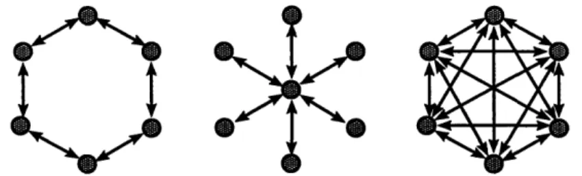
Most coupled oscillators in the natural world are organized in large networks, such as pacemaker cells in heart, neural networks in brain, fireflies with synchronized flashes, crickets with synchronized chirping, etc.[140, 144]. System (3.2) represents such an instance with a chain structure. In fact, there are many many other instances such as the three symmetric ones we illustrate in Figure 4-1.

(a)

1

-- 4 2 -3 (b) 1-4

1

--

4

2 -< >3

(c)

1 e~~ >4 12 >4 2~ 3

Figure 4-1: An n = 4 network with different symmetric structures.

In this chapter, we show that, partial contraction analysis can be applied to study the synchronization phenomenon in networked systems, not limited as oscillators, with various structures or arbitrary sizes. Either individual system's dynamics or coupling forces could be nonlinear.

4.1 Networks with All-To-All Symmetry

As the beginning, we study a network with all-to-all symmetry, that is, each element inside is coupled to all the others. Such a special example can be analyzed using an immediate extension of Theorem 3.2.

Theorem 4.1 Consider n coupled systems. If a contracting function h(xi, t) exists

such that

il - h(xl, t) * - t) f t= ch(ix

(34)

For instance, for identical oscillators coupled with diffusion-type force

n

xi = f(xi,t) + E (u(xj)-u(xi) )

j=l

(4.1)

contraction of f - nu guarantees synchronization of the whole network.

Example 4.1.1: Consider an all-to-all network containing four identical Van der Pol

oscillators

4

+ -(x? _ 1).t a2X, + = a.

D

-

)

j=l

i = 1,2,3,4 (4.2)

which can be re-written as

i = 1,2,3,4. .i + a(x/ + 4-).i + w2xi = any

Ej

j=l

Thus, these four oscillators will reach synchrony if > , for non-zero initial conditions. o~~~~~~~~~~~~~~~~~~

0

In [96], Mirollo and Strogatz study an all-to-all network of pulse-coupled integrate-and-fire oscillators, and derive a result on global synchronization. Their analysis is based on an event called absorption which is unique to all-to-all coupled networks.

4.2 Networks with Less Symmetry

Besides its direct meaning to all-to-all networks, Theorem 4.1 may also be applied to study networks with less symmetry.

Example 4.2.1: Consider an n = 4 network with two-way-ring symmetry (as illus-trated in Figure 4-1(b))

*i = f(xi,t) + (u(xi)-u(xi)) + (u(xi+)-u(xi)) where the subscripts i - 1 and i + 1 are computed circularly. oscillators into two groups (x1,x2) and ( 3, x4), we find

i = 1,2,3,4 Combining these four

*L - f(xi,t) + 2u(xi) = * -f(x 3,t) + 2u(x3) 1 = U(X2) + U(X4)

S - f(X 2,t) + 2u(X2) J L 4 -f(x 4,t) + 2u(x4) u(xl) + U(X3) J

Thus, if the function f- 2u is contracting, (l,x 2) converges to

and hence

{1

- ff(xl,t) + 2U(Xi) -- 2U(X2)

*k2 -f(x 2 ,t) + 2u( 2) -* 2U(Xi)

(X₃, X₄) exponentially,

so that in turn xi converges to x2 exponentially if the function f - 4u is contracting. The four oscillators then reach synchrony exponentially regardless of the initial conditions.

(35)

For four Van der Pol oscillators,

+ Ca(x~ -1) + w2x = aC ( ( i- -i) + (i+1 - ) )

a sufficient condition to reach synchrony is n >

(4.3)

[]

An extended partial contraction analysis can be used to study the example below, the idea of which will be generalized in the following section.

Definition 4.1 Consider n square matrices Ki of identical dimensions, and define

K 0 .. 0

In = 0 K2 .- 0

0 0 ... Kn One has IK > 0 if and only if Ki > , Vi.

Definition 4.2 Consider a square symmetric matrix K, and define

K K ... K K K ..- K

UK<=

. ...

K K ... K

nxn

One has UK > O if and only if K > O .

Example 4.2.2: Consider an n = 4 network with one-way-ring symmetry (as illus-trated in Figure 4-1(a))

x = f(xi,t) + K (xil - xi) i=1,2,3,4

where K = KT > 0 and the subscripts are calculated circularly. This system is equivalent to

4

xi = f(xi,t) - K(2xi +xi+1 +xi+2) + KExj

j=l

4

Construct an auxiliary system driven by the input K E xj (t)

j=l

4

yii=f(yi,t)-K(2yi+yi+1+Y i+2)+KExj(t) i=1,2,3,4

j=1

The auxiliary system admits the particular solution Yl = Y2 = Y3 = Y4 = yOC with 4

Y = = f(y.,t) - 4K y + KExj(t)

(36)

To apply Theorem 2.1 for the specific property Yl = Y2 = Y = Y4 and prove that all xi synchronize regardless of the initial conditions, there only remains to study the Jacobian matrix

J1 - 2K -K -K 0

j =0 J2 _J22K- _-KK -K

-K J3 - 2K 0 -K

-K -K 0 J4 - 2K

where Ji = (yi, t). The symmetric part of the Jacobian is

J1s-2K _K -K K K -K 2K J₂₈- 2K 2 -K Js = -K K 2 J38- 2K

-K

2 2 _Ji,,-K K -K ₂ _{_} _J 4s-2K =(IJ-K)--~ U 4K-- J+ where -K K J+ = K 0 K K K 0

We know that if Vi, Jis - K <0, then Ij K) < 0, and if K > 0 then UK > 0 and J+ > 0. If both conditions ae satisfied, the Jacobian Js is negative definite.

A corresponding Van der Pol example is

xi + a(x2- )i + w2xi = a±(il-i) i = 1, 2,3,4 (4.4)

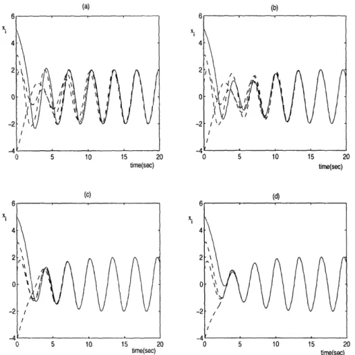
where the sufficient condition to reach synchrony asymptotically is > 1. 0 Note that up to now, we have studied the synchronization behaviors of coupled networks containing four oscillators with chain, one-way-ring, two-way-ring and all-to-all structures. Figure 4-2 lists simulation results of coupled Van der Pol oscillators, whose dynamics are based on equations (3.2), (4.4), (4.3) and (4.2). The asymptotic

1 1repcieyGieth

synchronization conditions are > 1, > 1, > , > , respectively. Given the same parameters ( = 0.5, w = 2, = 1.5) and the same initial conditions (chosen randomly), we see from the figures that the synchronization rate increases in such an order as

chain - one-way-ring -. two-way-ring -- all-to-all

We will explain this observation in Section 4.5. Note that in each figure, the ordinate is xi and the abscissa is time. The solid curve represents x1(t), the state of the first oscillator which is the independent one in the chain structure.

4.3 Networks with General Structure

Based on partial contraction analysis, we now study networked systems coupled in a very general structure. For notation simplicity, we first assume that coupling forces

(37)

(a)

time(sec) time(sec)

(c) _(d)

C 5 10 15 20

time(sec) 0 5 10 15 _time(sec)20

Figure 4-2: Four coupled Van der Pol oscillators synchronize with (a) chain, (b) one-way-ring, (c) two-way-ring, (d) all-to-all structure.

37 X. 4 2 0 .2 I/ H ., ,, (b)

(38)

are linear diffusive with gains Kij (associated with coupling from node i to j) positive definite, i.e., (Kij)8 = Kij8 > 0. We further assume that coupling links are

bidirec-tional and symmetric in different directions, i.e., Kij = Kji. All these assumptions can be relaxed as we will show later.

Consider now a network containing n identical elements

xi = f(xi, t) + E Ki (x - xi) i = 1,...,n (4.5)

jEAr

where Ni denotes the set of indices of the active links of element i. It is equivalent to

n n

= f(xt) + E Kji (xj-xi) - K0 Ex,+Ko x

jei j=1 j=1

where K0 is chosen to be a constant symmetric positive definite matrix (we will

discuss its function later). As usual, we construct an auxiliary system

n n

i = f(yi,t) + E Kji (Y - i)-Ko E Y + Ko E xj(t) (4.6)

jEAi j=1 5=1

which has a particular solution Y = Y = yoo with

n

yS = f(yc, t)-n Ko y + Ko E xj(t)

j=l

According to Partial Contraction Theory 2.1, if the auxiliary system (4.6) is con-tracting, all system trajectories will verify the independent property x = .-. = xn

exponentially.

Next, we compute J8, the symmetric part of the Jacobian matrix of the auxiliary

system.

Definition 4.3 Consider a square symmetric matrix K, and define

nxn

where all the elements in Tn except those already displayed in the four intersection points of ith and jth rows and ith and jth columns are zero. TK > 0 if K > O. Definition 4.4 Define the set

i = U iei

including a

including all the active links in the network.

n TK =

... K ... -K ... ... _K ... K

(39)

---Definition 4.5 Define

LK = E TnKij.

(i,j)EJ

In fact, if we view the network as a graph, LK is the symmetric part of the weighted Laplacian matrix [40]. The standard laplacian matrix is denoted as L.

Thus, we have

J = I. - LK - UK o

where Jis = ((yi, t))s.

Lemma 4.1 Define

Jr = -LK UKo

If K0 > 0 , Kij > 0, V(i, j) E JV, and the network is connected, then Jr < 0.

Proof: Note that each of the two parts in Jr is only negative semi-definite. Given an

arbitrary nonzero vector v = [v1,. .. vn]T_{, one has}

n n

VT Jr v = - (v-vj) Ki (v,- v- ( Vi)TKo (vi)

(i,j)EAr i=1 i

< 0

because the condition that the network is connected guarantees that vTJ r v= if and only if v1 =... = vn = -O.

Furthermore, the largest eigenvalue of Jr can be calculated as

Amax(Jr) = max v Jr = max( -vTLK-V vTUKov )

IlvII=1 I{viI=1

Since -vTUn v keeps decreasing as Ko increases except on the set i= vi 0, we

can choose Ko large enough and get

Amax(Jr) =- min vTLKv = -Am+1(LK)

Ilvll=l

I1v1I=1

=1Vi=°

according to the Courant-Fischer Theorem [51] - note that K0 is a virtual quantity

used to make Jr < 0 in the partial contracting analysis, and thus it cannot affect the real system's synchronization rate. Here the eigenvalues are arranged in an increasing

order, and A(LK) = = Am(LK) = 0, where m is the dimension of each individual

element.

Note that in the particular case m = 1, and VKj = 1, eigenvalue A2(LK) = A2(L)

is a fundamental quantity in graph theory named algebraic connectivity [34], which is equal to zero if and only if the graph is not connected. 0

(40)

The above results imply immediately

Theorem 4.2 Regardless of initial conditions, all the elements within a generally

coupled network (4.5) will reach synchrony or group agreement exponentially if

Am+l(LK) > max Amax(Jis) uniformly (4.7)

or, in words, if

* the network is connected,

* Amax(Jis) is upper bounded,

* the coupling strengths are strong enough.

Proof: The auxiliary system (4.6) is contracting if the condition (4.7) is true. 0

A few remarks on Theorem 4.2:

* The conditions given in Theorem 4.2 to guarantee synchronization represent the requirements on both individual system's internal dynamics and the network's geometric structure. A lower bound on the corresponding threshold of the coupling strength can be computed through eigenvalue analysis if a special network is given.

* Theorem 4.2 can also be used to find the threshold for symmetric subgroups in a network to reach synchrony, such as what we have illustrated in the simple Example 4.2.1.

* Partial contraction analysis does not add any restriction on the uncoupled dy-namics f(x, t) other than requiring Amax(Jis) to be upper bounded, which is easy to be satisfied if for instance individual elements are oscillators. As an example, Amax(Jis) = a for the Van der Pol oscillator. In fact, different

quali-tative choices exist for f, which can be an oscillator, a contracting system, zero, or even a chaotic system [113, 133, 144]. For a group of contracting systems, if

E

= I, the contraction property of the overall group will be enhanced by the diffusion couplings, and all the coupled systems are expected to converge to a common equilibrium point exponentially if f is autonomous. If L I,

how-ever, the situation is more complicated. A transformation process must be done in order to guarantee exponential convergence of the virtual dynamics. The cou-pling gain may lose positivity through the transformation, and the stability of the equilibrium point may be destroyed with strong enough coupling strengths. This kind of bifurcation is interesting especially if the otherwise silent systems behave as oscillators after coupling, a phenomenon of Smale's cells [79, 136, 153]. A simple example when n = 2 has been discussed in Section 3.2.2.

Contraction and partial contraction : a study of synchronization in nonlinear networks

Contraction and Partial Contraction:

Synchronization in Nonlinear Networks

by

Wei Wang

B.S., Thermal Engineering (1994)

Tsinghua University

M.S., Thermal Engineering (1997)

MAY 0 5 2005

LIBRARIES

Tsinghua University

Submitted to the Department of Mechanical Engineering

in partial fulfillment of the requirements for the degree of

Doctor of Philosophy in Mechanical Engineering

at the

MASSACHUSETTS INSTITUTE OF TECHNOLOGY

February 2005

©

Massachusetts Institute of Technology 2005. All rights reserved.

Author ...

...

...

Department of Mec anical Engineering

December 16, 2004

Certified by ... ...

...

...

Jean-Jacques E. Slotine

Professor of Mechanical Engineering and Information Sciences;

Professor of Brain and Cognitive Sciences

'/

Supervisor

Accepted by... ...

Lallit Anand

Chairman, Department Committee on Graduate Students

a Study of

Contraction and Partial Contraction: a Study of

Synchronization in Nonlinear Networks

by

Wei Wang

Abstract

Acknowledgments

Contents

List of Figures

En=

Chapter 1

Introduction

Chapter 2

Contraction and Partial

Contraction

2.1

Contraction Theory

116x1

2.2

Feedback Combination of Contracting Systems

dt

2.3

Partial Contraction Theory

$

]

{

+

d

)6 (4+

)

4 tends to

2.4

Line-Attractor

2.4.1

Line-Attractor

2.5

Appendix: Contraction Analysis of (2.5)

r

=

=

=

E-n_-=

=

+

2

_{+ dt)}

₊

_0((dt)')