Aggregative risk analysis for water quality failure in distribution networks

Publisher’s version / Version de l'éditeur:

Journal of Water Supply Research and Technology : Aqua, 53, May 4, pp. 241-261, 2004-05-01

READ THESE TERMS AND CONDITIONS CAREFULLY BEFORE USING THIS WEBSITE.

https://nrc-publications.canada.ca/eng/copyright

Vous avez des questions? Nous pouvons vous aider. Pour communiquer directement avec un auteur, consultez la

première page de la revue dans laquelle son article a été publié afin de trouver ses coordonnées. Si vous n’arrivez pas à les repérer, communiquez avec nous à PublicationsArchive-ArchivesPublications@nrc-cnrc.gc.ca.

Questions? Contact the NRC Publications Archive team at

PublicationsArchive-ArchivesPublications@nrc-cnrc.gc.ca. If you wish to email the authors directly, please see the first page of the publication for their contact information.

NRC Publications Archive

Archives des publications du CNRC

This publication could be one of several versions: author’s original, accepted manuscript or the publisher’s version. / La version de cette publication peut être l’une des suivantes : la version prépublication de l’auteur, la version acceptée du manuscrit ou la version de l’éditeur.

Access and use of this website and the material on it are subject to the Terms and Conditions set forth at Aggregative risk analysis for water quality failure in distribution networks

Sadiq, R.; Kleiner, Y.; Rajani, B. B.

https://publications-cnrc.canada.ca/fra/droits

L’accès à ce site Web et l’utilisation de son contenu sont assujettis aux conditions présentées dans le site LISEZ CES CONDITIONS ATTENTIVEMENT AVANT D’UTILISER CE SITE WEB.

NRC Publications Record / Notice d'Archives des publications de CNRC:

https://nrc-publications.canada.ca/eng/view/object/?id=5c3dc150-bbfd-4d57-8b69-04f33b2d6843 https://publications-cnrc.canada.ca/fra/voir/objet/?id=5c3dc150-bbfd-4d57-8b69-04f33b2d6843

Aggregative risk analysis for water quality failure in distribution networks

Sadiq, R., Kleiner, Y., Rajani, B.

NRCC-46269

A version of this document is published in / Une version de ce document se trouve dans : Journal of Water Supply Research and Technology : Aqua, v. 53, no. 4, May 2004, pp. 241-261

Aggregative Risk Analysis for Water Quality Failure in Distribution

Networks

1_{*Rehan Sadiq,} 2_{Yehuda Kleiner, and} 3_{Balvant Rajani}

1*: Research Officer

Institute for Research in Construction, National Research Council (NRC), M-20, 1200 Montreal Road

Ottawa, ON, Canada K1A 0R6 Rehan.sadiq@nrc-cnrc.gc.ca Phone: 1-613-993-6282 Fax: 1-613-954-5984

2: Senior Research Officer and Group Leader

Institute for Research in Construction, National Research Council (NRC), M-20, 1200 Montreal Road

Ottawa, ON, Canada K1A 0R6 Yehuda.Kleiner@nrc-cnrc.gc.ca Phone: 1-613-993-3805

Fax: 1-613-954-5984 3: Senior Research Officer

Institute for Research in Construction, National Research Council (NRC), M-20, 1200 Montreal Road

Ottawa, ON, Canada K1A 0R6 Balvant.Rajani@nrc-cnrc.gc.ca Phone: 1-613-993-3810 Fax: 1-613-954-5984

Abstract

The pathways, through which water quality in the distribution network can be compromised, may be classified into five categories: intrusion of contaminants into the distribution system (e.g., through cross connection), regrowth of bacteria in pipes and distribution storage tanks, water treatment breakthrough, leaching of chemicals or corrosion products from system

components (pipes, tanks, liners, etc.) and permeation of organic compounds through plastic pipe and pipe components in the system.

Quantification and characterization of the various risk factors in water distribution systems is a difficult task. Many kilometers of pipes of different ages and materials, uncertain operational and environmental conditions, unavailability of reliable data, and lack of understanding of some factors and processes affecting pipe performance make it extremely challenging. It is often difficult to identify or validate specific cause(s) for water contamination or waterborne disease outbreak because real-time data are rarely, if ever, available. For these reasons, high

uncertainties are inherent in any risk measure that may be assigned to the distribution system. Further, the current inability to precisely quantify most of these risks may warrant the usage of a quantitative-qualitative framework.

In this paper, a framework is presented for the analysis of aggregative risk associated with water quality failure in the distribution system. Each risk item is defined by the product of the

likelihood of a failure event and its consequence (peril). Both the likelihood and the

consequences of a failure event are defined using fuzzy numbers to capture vagueness in the qualitative linguistic definitions. A multi-stage hierarchical model of aggregative risk for water quality failure is developed. An analytic hierarchy process is used for estimating the priority matrix (weights) for grouping risk attributes. The framework is applied on a simplified structure of risk hierarchies for a water distribution system.

______________________________________________________________________________ Key Words: Distribution networks, fuzzy-based methodology, qualitative modeling, risk,

Introduction

The safety of drinking water is the supreme priority of water utilities and other water industry stakeholders. Total water quality management (TWQM) using multi-barrier approach (Health Canada 2002) and hazard analysis critical control points (HACCP) (Hulebak and Schlosser 2002) are two main concepts gaining popularity in the management of drinking water. A typical modern water supply system comprises the water source (aquifer or surface water source

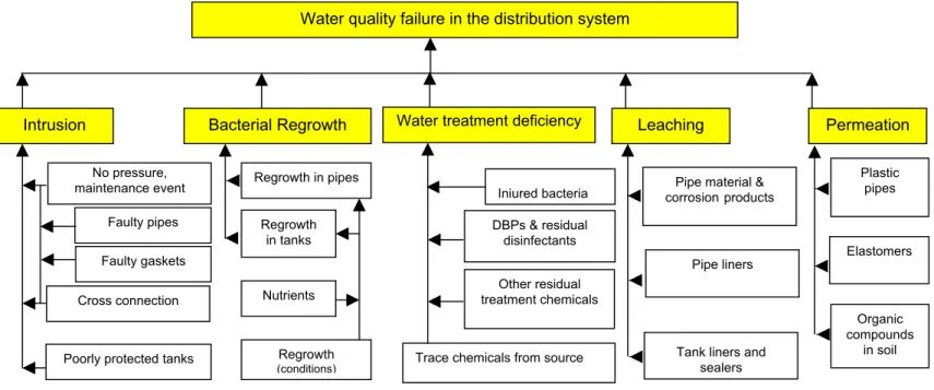
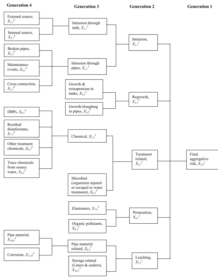
including the catchment basin), transmission mains, treatment plant and distribution network which includes pipes and distribution tanks. While water quality can be compromised at any component, failure at the distribution level can be extremely critical because it is closest to the point of delivery and, with the exception of a rare filtering device at the consumer level, there are virtually no safety barriers before consumption. Water quality failures (compromising either the safety or the aesthetics of water) in distribution networks can generally be classified into the following major categories (Kleiner 1998), also schematically described in Figure 1:

Intrusion of contaminants into the distribution system through system components whose integrity was compromised or through misuse;

Regrowth of microorganisms in the distribution network;

Microbial (and chemicals) breakthrough and byproducts and residual chemicals from water treatment plant;

Leaching of chemicals and corrosion products from system components into the water; and Permeation of organic compounds from the soil through system components into the water

supplies.

The quantification of contamination risk in water distribution systems is a difficult task. Water distribution systems comprise many (sometimes thousands) of kilometers of pipes of different ages and various materials. The operational and environmental conditions are highly variable and particularly dependent on pipe location. Further, pipes are buried structures, therefore limited performance and deterioration data are available. Finally, some of the failure processes are not well understood and forensic investigation of contamination is very difficult for water

distribution system because there is generally a time lag between the time of failure and the time at which the consequences (e.g., outbreaks) are observed.

Rowe (1977) defines risk as the potential for unwanted negative consequences of an event or an

activity, whereas Lawrence (1976) defines it as a measure of probability and severity of negative adverse effects. In this context, risk analysis is the estimation of the frequency and physical consequences of undesirable events, which can produce harm (Ricci et al. 1981). Therefore, risk

refers to the joint probabilities of an occurrence of an event and its consequences. When a complex system involves various contributory risk items with uncertain sources and magnitudes, it often can not be treated with mathematical rigor during the initial or screening phase of

decision-making (Lee 1996).

The objective of this paper is to describe a hierarchical model for the evaluation of an aggregative (cumulative) risk of water quality failure in distribution network. The model is termed hierarchical because it permits the breakdown of the aggregate risk in terms of the individual risk items. A qualitative (linguistic) modeling technique that combines fuzzy set theory with analytic hierarchy process (AHP) is proposed. Water quality deterioration caused by various internal and external sources is incorporated in the proposed model. The benefits as well as the limitations of this approach are discussed with recommendations for future research. In the following sections, some fundamentals of fuzzy set theory (FST) are presented, and a generic hierarchical structure model for aggregative risk analysis and knowledge acquisition process is also discussed. Later in this paper, the proposed framework is applied to water quality failure in distribution networks using a simplified structure of risk hierarchies to demonstrate its scope of application. The benefits and limitations of the proposed framework as well as

recommendations for future research are also discussed. Summary and conclusions of this research are provided in the end.

Soft Computing: Fuzzy-based Risk Concept

The term soft computing describes an array of emerging techniques such as fuzzy logic, probabilistic reasoning, neural networks, and genetic algorithms. All these techniques are essentially heuristic which provide rational, reasoned out solutions for complex real-world

problems (Bonissone 1997). Quantitative aggregation of risk due to various sources is a complex process, which warrants such an approach.

Fuzzy logic provides a language with syntax and semantics to translate qualitative knowledge into numerical reasoning. In many engineering problems, the information about the probabilities of various risk items is vaguely known or assessed. The term computing with words has been introduced by Zadeh (1996) to explain the notion of reasoning linguistically rather than with numerical quantities. Such reasoning has a central importance for many emerging technologies related to engineering and applied sciences.

When evaluating risk items in complex systems, decision-makers, engineers, managers,

regulators and other stake-holders often view risk in terms of linguistic variables like very high,

high, very low, low etc. The fuzzy set theory is able to deal effectively with these types of

uncertainties (encompassing vagueness), and linguistic variables can be used to approximate reasoning and subsequently manipulated to propagate the uncertainties throughout the decision process. Fuzzy-based techniques are a generalized form of interval analysis used to address uncertain and/or imprecise information. A fuzzy number describes the relationship between an uncertain quantity x and a membership function µ, which ranges between 0 and 1. A fuzzy set is an extension of the traditional set theory (in which x is either a member of set A or not) in that an

x can be a member of set A with a certain degree of membership µ. Fuzzy-based techniques can help in addressing deficiencies inherent in binary logic and are useful in propagating

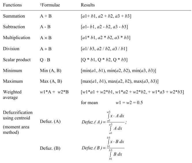
uncertainties through models. Any shape of a fuzzy number is possible, but the selected shape should be justified by available information. Generally, triangular fuzzy numbers (TFN) or trapezoidal fuzzy numbers (ZFN) are used for representing linguistic variables (Lee 1996). Table 1 provides commonly used arithmetic operations for two TFNs A and B. Details of these

arithmetic manipulations are described by Klir and Yuan (1995). Defuzzification is a process to evaluate a crisp or point estimate of a fuzzy number. A defuzzified number is generally

represented by centroid, often determined using the moment of area method (Yager 1980). Let the likelihood r of failure be defined by the triangular fuzzy number TFNr and the consequence (or peril) l of failure be defined by TFNl. The table in Figure 2 describes an 11-grade (or 11-granulars) qualitative scaling system for both factors r and l (as suggested by

Lee 1996). This 11-grade scale for likelihood includes absolutely low, extremely low, quite low,

low, mildly low, medium, mildly high, high, quite high, extremely high and absolutely high. In

addition, to represent a nil event i.e., if some phenomenon is surely absent, the q may be assigned a value of 0. For example if water distribution system does not have plastic pipes and other plastic components, likelihood of permeation will be 0. Similarly, an 11-grade scale for peril includes absolutely unimportant, extremely unimportant, quite unimportant, unimportant, mildly

unimportant, neutral, mildly important, important, quite important, extremely important and absolutely important. The objective of using 11-grade scale is to provide a decision-maker more

flexibility in expressing linguistic notions of likelihood and consequences (peril)

comprehensively. The membership functions of r and l to their respective granulars are defined as:    ≤ ≤ < ≤ − = , 1 x 1 . 0 , 0 , 1 . 0 x 0 , x 10 1 ) x ( or ) x ( _{r 1}l _l r 1 µ µ (q = 1) ) x ( _r r q µ or µ_ql(x_l )            ≤ ≤ ≤ ≤ − − − ≤ ≤ − − − − ≤ ≤ = , 1 x 10 q , 0 , 10 q x 10 1 q , x 10 q , 10 1 q x 10 2 q ), 2 q ( x 10 , 10 2 q x 0 , 0 (q = 2, 3, …10) (1) ) x ( _r r 11 µ or µ₁₁l (x_l ) (q = 11)    ≤ ≤ − ≤ ≤ = . 1 x 9 . 0 , 9 x 10 , 9 . 0 x 0 , 0

where xr is a continuous (latent) but uncertain variable for r, µqr(xr) is the function defining the membership of xr to granular q, xl is a continuous (latent) variable for l, µql(xl) is the function defining the membership of xl to granular q, and q denotes a granular (or a scale variable, or grade) of the fuzzy numbers. Figure 2 provides a graphical illustration of the relationships between the fuzzy numbers, their granulars and their membership functions. In the example of Figure 2, if the continuous uncertain number x “more mildly low (mildly unimportant) than

medium (neutral)” (i.e. approximately 0.43), has membership value of 0.70 to grade 5 (mildly low or mildly unimportant) and 0.30 membership value to grade 6 (medium or neutral). It implies

that likelihood/peril is 70% mildly low and 30% medium. The TFN definitions can be changed or modified based on expert recommendations or on Delphi method-based surveys (Lee and Kim, 2001).

Failure risk is defined as the product of the fuzzy numbers denoting r and l (see Table 1 for the definition of the product of two TFNs), which is equivalent to defining risk as the joint

probabilities of occurrence and consequences provided the representative probabilities are independent. By definition, the product of two TFNs is itself a TFN. Let TFNr be defined by the members (ar, br, cr) and TFNl by (al, bl, cl). The risk TFNrl for these r and l is then calculated by

TFNrl = TFNr× TFNl = (ar * al, br * bl, cr * cl) (2) The membership function µrl(xrl) of TFNrl is defined in the interval (ar * al) ≤ xrl≤ (cr * cl). In line with using qualitative linguistic variables, a scale system for risk is discretized in seven grades (or granulars), namely, extremely low (EL), quite low (QL), low (L), medium (M), high (H), quite high (QH) and extremely high (EH). For simplicity these risk granulars are denoted L1 through L7, respectively. Failure risk obtained in (equation 2) cannot be directly mapped into the 7-grade risk scale described above because it is derived from two TFNs with 11 granulars each. Instead, risk needs to be defuzzified and then the defuzzified value remapped into the 7-grade risk scale using the appropriate membership functions.

Various techniques for defuzzification are available, the most common of which are - Chen’s ranking (1985) and Yager’s centroid (1980) methods. In this paper, the centroid method is used for defuzzification due to its simplicity.

Defuzzified risk = ( ) ( ) ( ) ( ) ∫ ∫ ⋅ = l c * r c l a * r a rl rl l c * r c l a * r a rl rl rl dx ) x ( dx ) x ( x ) l , r ( g µ µ (3)

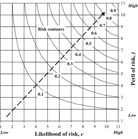
Figure 3 depicts the risk contours representing g(r,l) for all possible combinations of r and l. As can be expected, these contours show risk values that are increasing from left to right and bottom to top (i.e., with the increase in either likelihood or peril, individually or simultaneously).

These defuzzified risk factors g(r,l) now need to be mapped into the 7-grade risk scale described above. The membership function of this 7-grade risk scale is defined by

      ≤ ≤ ≤ ≤ − = , 1 x 6 1 , 0 , 6 1 x 0 , x 6 1 ) x ( _L L 1 µ            ≤ ≤ ≤ ≤ − − − ≤ ≤ − − − − ≤ ≤ = , 1 x 6 p , 0 , 6 p x 6 1 p , x 6 p , 6 1 p x 6 2 p ), 2 p ( x 6 , 6 2 p x 0 , 0 ) x ( _L L p µ (p = 2, 3, 4, 5, 6) (4)       ≤ ≤ − ≤ ≤ = . 1 x 6 5 , 5 x 6 , 6 5 x 0 , 0 ) x ( _L L 7 µ

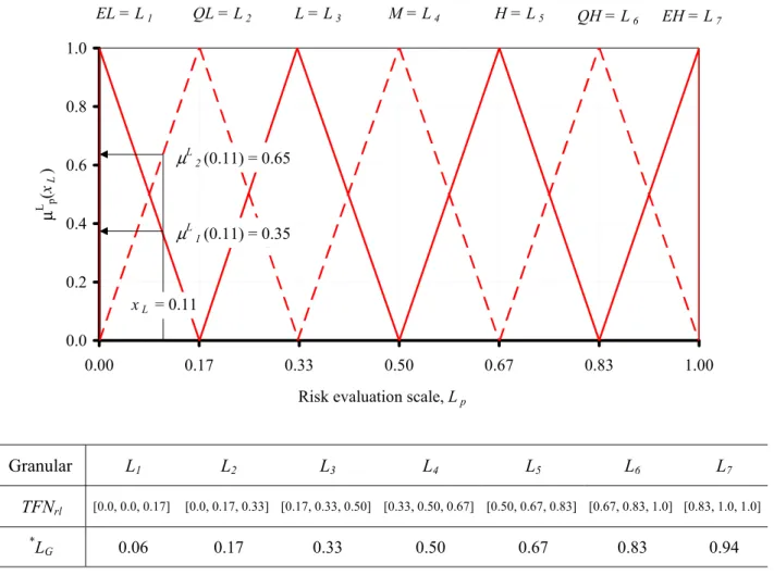
where xL = g(r,l) is the continuous (latent) variable for risk, and µpL(xL) is the function that defines the membership of xL to granular p. Figure 4 shows a graphical representation of the risk granulars, their TFNs and membership functions. Mapping of the continuous number xL into this 7-grade fuzzy risk scale requires another fuzzy set, which expresses the membership value of xL to each of the seven granulars in the system. For the example given in Figure 4, the membership values of xL = 0.11 to L1 and L2 are 0.35 and to 0.65, respectively. The fuzzy number

representing xL is the 7-tuple fuzzy set X= {0.35, 0.65, 0, 0, 0, 0, 0}, in which each tuple

represents the membership value of xL to each of the seven granulars in the system. This set can also take the notation

      = EH 0 , QH 0 , H 0 , M 0 , L 0 , QL 65 . 0 , EL 35 . 0

X , where the denominators are the

names of the corresponding granulars. Note that equation 4 dictates that the sum of memberships to the various granulars is unity (normalized fuzzy membership), however, this was done for convenience and cardinality of fuzzy sets does not require that this condition be essential.

The Hierarchical Structure Model and Risk Aggregation

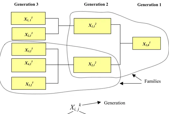
Figure 5 and Table 2 illustrate the basic building blocks of the hierarchical structural model. Essentially, each risk item is partitioned into its contributory factors which are also risk items, and each of those can be further partitioned into lower level contributory factors. The unit consisting of a risk factor (“parent”) and its contributory factors (“children”) is called “family”. A family consists of two generations but each of the children can be further partitioned into children of the next generation. A risk element with no children is called “basic risk item”, while the term risk item or risk attribute are interchangeably used for all elements with offspring. The notation for a risk item or attribute is Xi,jk, where i is the ordinal number of risk item X in the current generation; j is the ordinal number of the parent (in the previous generation); and k is the generation order of X. In Table 2, the factors ri,jk and li,jk respectively denote likelihood and peril for the risk item Xi,jk. When the respective contributions of sibling risk items towards their parent are non-commensurate in their units (e.g., one is quantified as financial loss, while the other in terms of environmental damage), a weighting scheme is required. Table 2 shows the general case where weights are assigned to each risk item. The notation used is Wi,jk, where W denotes the weight of Xi,jk relative to its siblings. The weights are estimated using analytic hierarchy process (AHP) and the details are given in the following paragraphs. When the respective contributions of sibling risk items towards their parent are commensurate in their units, then Wi,jk are equal for all the siblings.

The analytic hierarchy process (AHP) is a technique commonly used for multiple-criteria analysis. The AHP develops a linear additive model, which derives weights by performing pair-wise comparisons between criteria or attributes (Ziara et al. 2002). Table 3 depicts a 9-level scale of relative importance used in this process of pair-wise comparisons. The comparison results are then arranged into a reciprocal matrix (Saaty 1996; Sadiq et al. 2003) which is subsequently used to calculate the implied weights. These weights are normalized to a sum of 1, such that in any generation (k), for n siblings for a given parent j, a set of weights Wkj can be written as

) W ..., , W , W ( W_jk = _1,jk _2,jk _n,jk where ∑ = (5) = n 1 i k j , i 1 W

Saaty (1988, 2001) describes full details of the procedure to derive weights from relative importance scale.

Aggregation of fuzzy sets require operations by which several fuzzy numbers are combined in a desirable way to produce a single fuzzy number (Klir and Yuan 1995). The literature reflects numerous ways and operators to aggregate fuzzy sets, e.g., intersection, minimum, product (also known as fuzzy t-norms) and union, maximum, summation (also known as s-norms). The

aggregation process in fault tree analysis uses probabilistic type of intersections (and gate) and unions (or gate) (e.g., see Khan et al. 2002). Other common operators for aggregation are

arithmetic, geometric and harmonic means. In addition, there is a class of averaging operators, generalized means, which provides flexible aggregation operators ranging between the minimum

and the maximum operators. Another class of aggregation operators includes the ordered

weighted averaging operators (OWA). Detailed discussions on the selection of appropriate

aggregation operators are given by Klir and Yuan (1995), and Smolikova and Wachowiak (2001). In this study, the weighted average technique was used to aggregate risk.

The process of evaluating aggregative risk in a fundamental unit (i.e., “family”) of the

aggregative structure can now be summarized, using the family (Figure 5) of X2,12 (parent) and

X3,23, X4,23, X5,23(children) as an example. For each of the sibling risk items the likelihood r and peril l are estimated using the 11-grade scaling system in Figure 2. Their respective TFNr and

TFNl values are then multiplied to obtain their TFNrl values (equation 2), which are then defuzzified using equation (3) to obtain the respective values for g(r,l). These values are then mapped into the 7-grade risk scale (Figure 4), using equation (4) to obtain the 7-tuple fuzzy sets

X3,23, X4,23, X5,23representing the risk contribution of each of the siblings towards their parent. For ease of manipulation these 7-tuple fuzzy sets can be arranged in a fuzzy assessment matrix (FAM), which is a 3 × 7 matrix F(Xi,23), where the index j = 2 stands for siblings of parent item number 2 in the previous generation. The analytic hierarchy process (AHP) is then applied and weights W3,23, W4,23, W5,23are evaluated and arranged into a 3-member vector. The aggregative risk (or parent or risk attribute) of the three siblings is a 7-tuple fuzzy set X2,12which is calculated by regular matrix multiplication

[

]

[

]

where µpL (p = 1, 2,…, 7) are the membership values of the aggregated risk to the granulars of the 7-grade risk scale. The aggregation of risk towards the next level (next generation) is done in the same way, i.e., evaluating the appropriate weight vectors and multiplying by FAM.

It should be pointed out here that the process of evaluating r and l and re-mapping the product

risk into the 7-grade risk scale, is done only for basic risk items (those risk items which do not have children). Consequently it is useful to use notation that distinguishes between basic and non-basic risk items. In the remainder of this paper, the notation for a basic risk item will include an apostrophe at the generation index, i.e., if item X4,23 is a basic risk item, it will be denoted

X4,23’. It should also be noted that in the first generation of the structure (i.e., the head of the pyramid) the final aggregative risk can be defuzzified to provide a single (crisp) measure of the risk of the entire structure. This can be done by

Defuzzified risk = L_G⋅X_1,01 (7)

where LG is the 7-member vector defined in Figure 4. The defuzzified risk is calculated as a dot product of vector LG and fuzzy number X1,01.

Knowledge Acquisition

Knowledge acquisition is required to explore and develop relationships between basic risk items and events of occurrence. For example, the age of a pipe can be associated with its breakage rate and thus to the likelihood of contaminants’ intrusion in case of maintenance events. Similarly, contamination due to treatment breakthrough can be associated with the treatment method, demand in peak hours, etc. Knowledge acquisition consists of four distinct activities: preliminary analysis; literature review; surveys/interviews and solicitations of opinions of an expert panel. The preliminary analysis helps to obtain an overview of the problem and determine potential modular categories that would be useful in classifying various types of risks. The preliminary analysis breaks down the risk items along categorical lines, which help identify contributory risk factors (McCauley-Bell and Badiru 1996). For water quality in distribution networks this

analysis could be carried out along the contamination pathways as illustrated in Figure 1. An in-depth literature review follows the preliminary analysis. The result of this analysis provides a

more comprehensive understanding of risk items associated with water quality. With a more comprehensive understanding, questionnaires and interview sessions can be designed to query the knowledge of utility personnel and other professionals working in the water industry. Finally, an expert panel is assembled to discuss and organize the available information as well as to help fill identified knowledge gaps. The final data of basic risk items may be qualitative, quantitative or a hybrid of both.

An Application of the Proposed Methodology – A Hypothetical Case Study Water quality failure

Intrusion of contaminants in the water distribution system can occur through pipes and storage tanks. Open finished water reservoirs are susceptible to microbial contamination from external non-point sources such as feces of infected animals, e.g., beaver, squirrels and rabbits, within the watershed. Microorganisms can be introduced into open reservoirs from windblown dust, debris, and algae. Organic matter (leaves and pollens) are also of concern in open storage tanks

(Kirmeyer et al. 2001). Finished water can also be affected in covered facilities by airborne

microorganisms entering through access hatches, overflow pipes and vents, roofs and side walls (Kirmeyer et al. 2001). Microorganisms can also be introduced into ground level storage through

surface water (flooding) or groundwater infiltration. Bird droppings are commonly found in storage facilities with floating covers (Clark et al. 1997).

Intrusion of contaminants through water mains may occur during maintenance and repair events, through broken pipes and gaskets, and cross connections. A broken gasket that seals pipe joints can be a pathway for variety heterotrophic bacteria in the distribution network (Geldreich 1990). Regular maintenance and repair events as well as other anthropological and natural disasters may cause intrusion of contaminants in the water distribution network.

Cross connections (an unprotected physical connection between a potable and a non-potable water system) can potentially introduce substances that may compromise the quality of potable water. Backflow from cross connections may occur when the pressure inside the water main is less than the pressure at the entry point. This can happen when a water main breaks and is de-pressurized for breakage repair, or when peak demands occurs, or when an outside de-pressurized

source is connected to the potable water system or without backflow protection (Kirmeyer et al.

2001). Contamination events can also occur as a result of transient pressures in the distribution system, where negative or low pressures cause backflow into distribution mains.

Biofilm is defined as a deposit consisting of microorganisms, microbial products and detritus at the surface of pipes or tanks. Biological regrowth occurs when injured bacteria pass from the treatment plant into the distribution system and subsequently rejuvenate and grow in storage tank, and water mains. The regrowth of organisms in the distribution system increases chlorine demand of the system, thus reducing the level of free chlorine, which may hinder the system’s ability to contend with local occurrences of contamination (US EPA 1999).

Disinfection is the primary method to inactivate pathogens. Chlorine has been highly successful in reducing the incidences of waterborne infections in human beings but other concerns have been raised in the last three decades about the safety of the disinfected water. Harmful

disinfection by-products (DBPs) are formed in the presence of natural organic matter (NOM) and bromide (from the source) during chlorination. Other commonly used disinfectants are

chloramines (combined chlorine), chlorine di-oxide and ozone. These disinfectants have different levels of effectiveness against disease causing pathogens. Ozone reacts with NOM and produces aldehydes, ketones and inorganic by-products. Ozone and chlorine di-oxide in the presence of bromide ion produce bromate, chlorate and chlorite, respectively, which may have adverse human health effects (US EPA 1999).

Recently, the presence of trace chemicals like endocrine disrupting compounds and pharmaceuticals in source water has raised long term health and environmental concerns (AwwaRF 2003). Several agencies including American Water Works Association Research Foundation (AwwaRF) are funding research related to the fate, occurrence and treatment of these compounds.

Permeation is a phenomenon in which the contaminants migrate through the pipe wall. Three stages are observed in physico-chemical process of permeation: (a) organic chemicals present in the soil partition between the soil and plastic wall, (b) the chemicals defuse through the pipe wall, and (c) the chemicals partition between the pipe wall and the water inside the pipe (Kleiner 1998). Holsen et al. (1991) has reported that most of the permeation events occur where the soil

is contaminated with gasoline, diesel fuel, or solvents. Thompson and Jenkins (1987) have reported that polyethylene pipes are potentially susceptible to permeation of non-polar organic compounds. Similarly, all elastomeric and thermo-plastic materials are prone to permeation. In general, the risk of contamination through permeation is relatively small compared to other mechanisms.

Red water is one the most common causes of water quality failure although the peril is a loss of aesthetics rather than health. The corrosion of metallic pipes and plumbing devices increases the concentration of metal compounds in the water. Different metals go through different corrosion processes, but in general low pH water, high dissolved oxygen, high temperature, and high levels of dissolved solids increase corrosion rates. Heavy metals such as lead and cadmium may also leach into the water from the pipe materials. Secondary metals such as copper (from home plumbing), iron (distribution pipes) and zinc (galvanized pipes) may leach into water and cause taste, odor and color problems in addition to minor health related risks (Kleiner 1998).

Contamination of water by compounds leached from pipe liners (plastic and epoxy lining) has also been observed. Aschengrau et al. (1993) has explored the exposure of perchloroethylene

(PCE) to human population and linked it to occurrence of cancer cases.

Kirmeyer et al. (2001) assembled an expert panel to rank pathogen (contaminant) entry. Each

member on the expert panel was given a number of votes and instructed to identify and rank (at three qualitative levels of low, medium and high) the most important routes of entry. Additional

routes of pathogen entry have been included in Table 4 to reflect different pipe materials and security concerns.

Figure 6 shows a simplified hierarchical structure for water quality failure. This structure is used to demonstrate the aggregative risk framework introduced earlier. Table 5 lists the 17 basic risk items for the proposed structure. These basic risk items are grouped into third generation risk attributes, which in turn are grouped into second generation risk attributes including intrusion, regrowth, water treatment related, permeation and leaching. A more elaborate structure could, for example, partition the basic risk item, broken pipes into pipe age groups, material, surrounding soil types etc. Similarly, risks due to disinfection by products (DBPs) can be broken down into specific species like trihalomethanes (THMs) and haloacetic acids (HAAs), and THMs can be

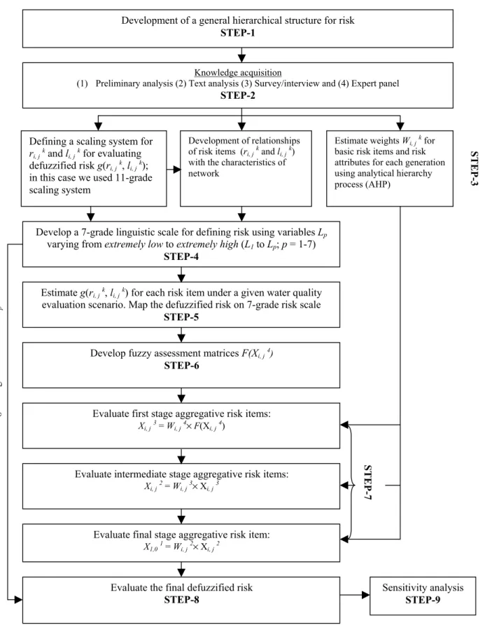
further broken down to chloroform, bromoform, etc. Various local and regional factors (e.g., geographical location, type of water treatment, climate, size and age of distribution system, soil/topography, rehabilitation and frequency of flushing programs and others) affect the magnitude of both r and l for each basic risk item. A step-by-step process for estimating

aggregative risk of water quality failure is shown in Figure 7. The weight matrices Wi,jk for each set of siblings were developed using an AHP technique as discussed in section 3. The estimated weights are summarized in Table 6.

First stage risk aggregation

The first stage aggregation process is applied only to basic risk items. For each basic risk item, r

and l are assigned q-grade value and then defuzzified risk g(ri,jk, li,jk) is obtained using Figure 3. This process is summarised in Table 5 for all the basic risk items in the suggested simplified structure. It should be noted that a basic risk item can be in any generation in the hierarchical structure. The g(ri,jk, li,jk) values are then mapped on the 7-grade risk scale (see Figure 4) to estimate their membership µpL(x) to the seven risk levels L1 to L7. For example, for basic risk

item X1,14’, the defuzzified risk value against g(5, 9) is equal to 0.325 (using Figure 3). The 0.325 value is mapped on Figure 4, and the memberships µpL(x) to the 7-grade risk scale are L1 = 0,

L2 = 0.05, and L3 = 0.95 and L4 to L7 = 0 (Table 7). The same procedure is applied to X2,14’ and subsequently, F(Xi,14) matrix can be formed as

      = 0 0 0 0 0 06 . 0 94 . 0 0 0 0 0 95 . 0 05 . 0 0 ) X ( F _i,14 (8)

After this process is applied to all the families which include basic risk items, the fuzzy risk assessment matrices F(Xi,24), F(Xi,23), F(Xi,54), F(Xi,33), F(Xi,43), F(Xi,94) and F(Xi,53) can be

established. These fuzzy risk assessment matrices are then multiplied by their respective weights. For example, F(Xi,14) is multiplied by weights W1,14 and W2,14 to determine risk item X1,13

[

] [

]

[

3 1

1 W W F(X ) . . .

Similarly, all the other first stage aggregative risk items can be determined. The risk items estimated in first stage aggregation can now be used to evaluate the aggregative risk items in the next stage.

Intermediate stage(s) risk aggregation

The intermediate stage risk aggregation is applied to all non-basic risk items except those feeding into the head of the pyramid. In the intermediate stage, the risk items from the previous stage are weighted and grouped to obtain the aggregated risk in the next generation. For example, X1,13 and

X2,13 are multiplied by W1,13 (= 0.33) and W2,13 (= 0.67) to obtain the intermediate risk item X1,12

[

]

[

]

]

All other intermediate risk items are determined following same steps. These risk items can now be used to evaluate the aggregative risk items in the final stage.

Final stage risk aggregation

To obtain the final risk item X1,01 (head of the pyramid), the intermediate stage aggregative risk items X1,12, X2,12, X3,12, X4,12 and X5,12 are arranged to form the fuzzy risk assessment matrices

F(Xi,12), which is then multiplied by the corresponding weights W1,12 (= 0.39), W2,12 (= 0.21),

W3,12 (= 0.20), W4,12 (= 0.07) and W5,12 (= 0.13)

[

]

[

X1,01 is the final aggregative risk item. It is a 7-tuple fuzzy set, which can be expressed as

      = EH 0 , QH 0 , H 01 . 0 , M 02 . 0 , L 30 . 0 , QL 35 . 0 , EL 33 . 0 X_1,01 (13)

Equation (13), also called a possibility mass function, is plotted in Figure 8. The final defuzzified aggregative risk is determined by the multiplication of the centroids of membership functions LG and the 7-tuple fuzzy set X1,01 as in equation (7). In this example, the final defuzzified risk is

. The results of the analyses are summarized in Table 7.

19 . 0 X L_G ⋅ _1,01 ≈ Discussion

In hierarchical (multiple-level) aggregation processes, recognition of two potential pitfalls namely exaggeration and eclipsing is important. Exaggeration occurs when all basic risk items are of relatively low risk, yet the final aggregative risk comes out unacceptably high. Eclipsing is the opposite phenomenon, where one or more of the basic risk items is of relatively high risk, yet the estimated aggregative risk comes out as unacceptably low. These phenomena are typically affected by the aggregation method used, thus the challenge is to determine the best aggregation method which will simultaneously reduce both exaggeration and eclipsing.

Aggregation operators used for the development of environmental indices generally include additive forms (simple addition, arithmetic average, weighted average), root sum power, root sum square, maximum, multiplicative forms (e.g., geometric mean, weighted product), and minimum operators (Silvert 2000; Somlikova and Wachowiak 2001; Ott 1978). Model predictions may be sensitive to both the types of aggregation operators as well as to weights. Generally, a sensitivity analysis (step 9 in Figure 7) is conducted to quantify the change in output caused by changes in input values. In the proposed framework the sensitivity analysis should be extended to examine the effects of weights and aggregation operators as well. A comprehensive sensitivity analysis will depend on the actual values of the specific case at hand. As the case study presented here is but a simplified example with hypothetical values, applying such a sensitivity analysis here would be of little value.

The application of the proposed hierarchical aggregative risk approach has several benefits and advantages:

• It enables the synthesis of both quantitative and qualitative information into a single framework;

• It can explicitly consider and propagate uncertainties inherent in linguistic expressions throughout the hierarchical structure;

• Its modular form is scalable; enabling it to accommodated new knowledge and information,

such as vulnerability to terrorist acts (safety related risk), hydraulic failure, financial risk etc.;

• It can be used to conduct cost-benefit analyses to facilitate effective budget allocation and prioritize attention required to components that have the most adverse impact on total system risk. For example, assume an aggregative risk of a water distribution system is evaluated as

low to medium but the level of “acceptable risk” is defined as quite low to low by a regulatory

agency. Furthermore, assume that it is found that two basic risk items are responsible for these higher risk values. The proposed hierarchical aggregative risk approach can then be used to re-evaluate if the “rehabilitation” of the two risk items will lead to a decrease in the

aggregative risk to an acceptable regulatory level of quite low to low. Subsequently, the costs

of both of these options can be examined and the most economical option can be selected for application.

• More data results in reduced uncertainty, which, when propagated through the hierarchical structure, can result in reduced uncertainty in aggregative risk. The proposed approach can help pinpoint areas where more data would yield increased benefits. For example, a basic risk item with very high peril (l) but very low likelihood (r) is not as good as a candidate for

further investigation as a risk item of medium peril and medium likelihood, even though the

risks of both items are likely to be similar.

• It is easily programmable for computer applications and can become a risk analysis tool for a water distribution system;

The limitations of the proposed method are:

• It may be sensitive to the selection of aggregation operators. Different operators can be used for different segments of the model. Trial and error approach may be required to avoid exaggeration and eclipsing; and

• This framework accommodates both qualitative and quantitative data. Some data may be supported by rigorous observations, while other data may be based on loosely supported or anecdotal-based beliefs. These two types of data should have different weights in the

aggregation process. The hierarchical structure in its current form does not address this need to distinguish between data obtained from sources of different reliabilities.

The structure presented in this paper is a simplified application of the approach. A

comprehensive structure would require a major effort, including the collaboration of several experts in the various disciplines of knowledge.

Summary and Conclusions

The water in distribution networks can be contaminated via several pathways. The quantification and characterization of the various risk factors in water distribution systems is a complex

process. Thousands of kilometers of pipes of different ages and materials, uncertain operational and environmental conditions, unavailability of reliable data, and lack of understanding of some factors and processes affecting pipe performance make it extremely challenging.

In this study, an approach is developed to estimate aggregative risk from various sources and pathways. Risk is defined as a product of likelihood and peril, where both factors are expressed in terms of qualitative scales (defined by fuzzy numbers). A modular hierarchical model is developed to provide a framework for aggregating risk items of water quality failure. An analytic hierarchy process is used for the aggregation of the risk factors. Weighted average operators are used for grouping various risk items and attributes that may be expressed in non-commensurate units. The selection of appropriate aggregation operators can be challenging. Future research should develop an elaborate system, including expert panels, and processes for the selection of the most appropriate aggregation operators.

In the model development stages, the final aggregative risk value is expected to have limited meaning for the acceptability of risk by public. It is envisaged that as this hierarchical structure is developed, populated and subsequently improved upon (using newly obtained data) the

developers will gain insight into risk levels as they are manifested in the final fuzzy and/or defuzzified risk values. Local and regional factors (e.g., geographical location, climate, size and

age of distribution system, soil/topography, rehabilitation and frequency of flushing programs and others) can be used to decide magnitude for both factors r and l for each basic risk item. In

the longer terms, this approach could serve as a basis for bench marking acceptable risks in water distribution system. In the future research, the authors of this paper will attempt to collect real data from different distribution systems to demonstrate the applicability of this approach. A similar hierarchical framework can be created where the values propagated up the structures are symptoms (e.g., minor illnesses) rather risk values. Such a framework could be used for diagnostic/forensic purposes, where for example, a number of reported minor illnesses could be attributed to the most likely cause, such as intrusion or microbial regrowth.

References

Aschengrau, A., Ozonoff, D., and Paulu, C. 1993 Cancer risk and tetrachloroethylene

contaminated drinking water in Massachusetts. Archives of Environmental Health 48(5),

227-230.

AwwaRF 2003. Pharmaceuticals Eendocrine Disrupting Compounds, and Personal Care

Products – Where Do We Go from Here?. Solicited projects proposed FY 2003. American

Water Works Association Research Foundation.

Bonissone, P.P. 1997 Soft computing: the convergence of emerging reasoning technologies. Soft Computing 1: 6-18.

Chen, S.H. 1985 Ranking fuzzy numbers with maximising set and minimising set. Fuzzy Set and

Systems 17(2), 113-129.

Clark, R.M., Reasoner, D.A., Fox, K.R., and Hurst, C.J. 1997 Drinking water treatment and distribution: its role in preventing waterborne outbreaks. Presented at Workshop on Design of Waterborne Disease Occurrence Studies, Atlanta, GA.

Geldreich, E.E. 1990 Microbiological quality control in distribution systems, In: Water Quality and Treatment. Edited by Frederick, W.P., American Water Works Association, NY, McGraw-Hill Inc.

Health Canada 2002 From Source to Tap – the Multi-barrier Approach to Safe Drinking Water.

http://www.hc-sc.gc.ca/hecs-sesc/water/publications/source_to_tap/source_to_tap-toc.htm, Health Canada.

Holsen, T.M., Park, J.K., Jenkins, D., and Selleck, R.E. 1991 Contamination of potable water by permeation of plastic pipe. JAWWA 83(8), 53-56.

Hulebak, K.L., and Schlosser, W. 2002 Hazard analysis and critical control point (HACCP) – history and conceptual overview. Society of Risk Analysis, Risk Analysis, 22(3), 547-552.

Khan, F.I., Sadiq, R., and Husain, T. 2002 Risk-based process safety assessment and control measures design for offshore process facilities. Journal of Hazardous Materials A94, 1-36.

Kirmeyer, G.J., Friedman, M., Martel, K., and Howie, D. 2001. Pathogen Intrusion into Distribution System. AwwaRF, Denver, CO, USA.

Kleiner, Y. 1998 Risk factors in water distribution systems. British Columbia Water and Waste Association 26th Annual Conference, Whistler, B.C., Canada.

Klir, G.J., and Yuan, B. 1995 Fuzzy Sets and Fuzzy Logic - Theory and Applications. Prentice-

Hall, Inc., Englewood Cliffs, NJ, USA.

Lawrence, W.W. 1976 Of Acceptable Risk. William Kaufmann, Los Altos, CA.

Lee, H.-M. 1996 Applying fuzzy set theory to evaluate the rate of aggregative risk in software

development. Fuzzy Sets and Systems 79, 323-336.

Lee, J.W., and Kim, S.H. 2001 An integrated approach for interdependent information system project selection. International Journal of Project Management 19(2), 111-118.

McCauley-Bell, P., and Badiru, A.B. 1996 Fuzzy modeling and analytic hierarchy processing to quantify risk levels associated with occupational injuries – Part I: the development of fuzzy linguistic risk levels. IEEE Transactions on Fuzzy Systems 4(2), 124-131.

Ott, W.R. 1978 Environmental Indices: Theory and Practice. Ann Arbor Science Publishers Inc.,

pp. 371.

Ricci, P.F., Sagen, L.A., and Whipple, C.G. 1981 Technological Risk Assessment Series E:

Applied Series No.81.

Rowe, N. 1977 Risk: An Anatomy of Risk. John Wiley and Sons, NY.

Saaty, T.L. 1988 Multicriteria Decision-Making: The Analytic Hierarchy Process. University of

Pittsburgh, Pittsburgh, Pa, USA.

Saaty, T.L. 1996 Decision Making with Dependence and Feedback: The Analytic Hierarchy

Process. RWS, Pittsburgh, Pa, USA.

Saaty, T.L. 2001 How to make a decision? Chapter 1, Models, Methods, Concepts and

Applications of the Analytic Hierarchy Process. Ed. Saaty, T.L., and Vargas, L.G., Kluwer

International Series.

Sadiq, R., Kleiner, Y., and Rajani, B. 2003 Water quality failure in distribution networks: a

framework for an aggregative risk analysis. American Water Works Association (AWWA)

Silvert, W. 2000 Fuzzy indices of environmental conditions. Ecological Modelling 130(1-3),

111-119.

Somlikova, R., and Wachowiak, M.P. 2001 Aggregation operators for selection problems. Fuzzy

Sets and Systems 131, 23-34.

Thompson, C., and Jenkins, P. 1987 Review of Water Industry Plastic Pipe Practices. AwwaRF,

Denver, CO.

US EPA 1999 Microbial and Disinfection By-product Rules – Simultaneous Compliance

Guidance Manual. United States Environmental Protection Agency, EPA 815-R-99-015.

Yager, R.R. 1980 A general class of fuzzy connectives. Fuzzy Sets and Systems 4, 235-242.

Zadeh, L.A. 1996 Fuzzy logic computing with words. IEEE Transactions – Fuzzy Systems, 4(2),

103-111.

Ziara, M., Nigim, K., Enshassi, A., and Ayyub, B.M. 2002. Strategic implementation of infrastructure priority projects: case study in Palestine. ASCE Journal of Infrastructure Systems, 8(1), 2-11.

List of Symbols

k Order of generation

j Order of parent with respect to previous generation

i Order of children in a given generation

l Peril (hazard)

r Likelihood (chance)

q Granular (or scale variable, or grade) of a fuzzy number representing r or l p Granular (or scale variable, or grade) of a fuzzy number representing risk level x Continuous (latent) variable, to be mapped into a fuzzy multi-grade system g(ri,jk, li,jk) Defuzzified risk (centroid) for a given likelihood and peril

µ(x) Membership function of continuous (latent) variable x Xi,jk Seven-tuple risk item and/or risk attributes

F(Xi,jk) Fuzzy assessment matrix

Lp Linguistic variables representing grades of risk (p = 1 to 7)

LG Centroid of qualitative scales Lp

Wi,jk Weight

TFNr, TFNl Triangular fuzzy numbers for likelihood, peril, respectively TFNL = TFNrl Triangular fuzzy numbers for risk

Aggre gative risk a nalysi s for wate r qu ali t Intrusion No pressure, maintenance event Cross connection Faulty pipes Faulty gaskets

Poorly protected tanks

Bacterial Regrowth Nutrients Regrowth (conditions) Regrowth in pipes Regrowth in tanks Leaching

Pipe material & corrosionproducts

Pipe liners

Tank liners and sealers Organic compounds in soil Elastomers DBPs & residual disinfectants Other residual treatment chemicals

Trace chemicals from source

Figure 1. Contamination pathways in water distribution systems (modified after Kleiner, 1998)

Plastic pipes

Permeation Water quality failure in the distribution system

Injured bacteria

Water treatment deficiency

y failure in distributio

n net

works

24

Granulars (q)* Qualitative scale for likelihood of risk (r)

Qualitative scale for peril of risk (l)

Triangular fuzzy numbers (TFNr or l)

1 Absolutely low Absolutely unimportant (0, 0, 0.1)

2 Extremely low Extremely unimportant (0, 0.1, 0.2)

3 Quite low Quite unimportant (0.1, 0.2, 0.3)

4 Low Unimportant (0.2, 0.3, 0.4)

5 Mildly low Mildly unimportant (0.3, 0.4, 0.5)

6 Medium Neutral (0.4, 0.5, 0.6)

7 Mildly high Mildly important (0.5, 0.6, 0.7)

8 High Important (0.6, 0.7, 0.8)

9 Quite high Quite important (0.7, 0.8, 0.9)

10 Extremely high Extremely important (0.8, 0.9, 1)

11 Absolutely high Absolutely important (0.9, 1, 1)

*q is assigned a value of “0”, in case of an absence of an event (i.e., likelihood/peril are nil)

0 0.2 0.4 0.6 0.8 1 0 0.1 0.2 0.3 0.4 0.5 0.6 0.7 0.8 0.9 1 Likelihood/Peril Membership function

Granular-1 Granular-5 Granular-6 Granular-11

x = 0.43 (more mildly low than medium)

µ5(0.43) = 0.70

µ6(0.43) = 0.30

... ...

1 2 3 4 5 6 7 8 9 10 11 1 2 3 4 5 6 7 8 9 10 11 Likelihood of risk, r Peril of risk, l 0.1 0.2 0.3 0.4 0.5 0.6 0.7 0.8 0.9 Risk contours Low Low High High

0.0 0.2 0.4 0.6 0.8 1.0 0.00 0.17 0.33 0.50 0.67 0.83 1.00

Risk evaluation scale, Lp

µ L p (x L ) EL = L1 QL = L2 L = L3 M = L4 H = L5 QH = L6 EH = L7 xL = 0.11 µL 1(0.11) = 0.35 µL 2(0.11) = 0.65 Granular L1 L2 L3 L4 L5 L6 L7 TFNrl [0.0, 0.0, 0.17] [0.0, 0.17, 0.33] [0.17, 0.33, 0.50] [0.33, 0.50, 0.67] [0.50, 0.67, 0.83] [0.67, 0.83, 1.0] [0.83, 1.0, 1.0] * LG 0.06 0.17 0.33 0.50 0.67 0.83 0.94

*LG is the x-co-ordinate of the centre of gravity of a granular and is expressed as a vector LG = {0.06, 0.17, 0.33, ... , 0.94}

Generation

X

Leaching,

X5,12

Storage related (Liners & sealers),

X10,5 3’ Pipe material related, X9,53 Intrusion through tank, X1,13 Corrosion, X11,94’ Pipe material, X10,9 4’ Permeation, X4,12 Regrowth, X2,12 Organic pollutants, X8,4 3’ Elastomers, X7,43’ Treatment related, X3,12 Intrusion, X1,12 Final aggregative risk, X1,01 Microbial (organisms injured or escaped in water treatment), X6,33’ Trace chemicals from source water, X9,54’ Other treatment chemicals, X8,54’ Chemical, X5,33 Residual disinfectants, X7 5 4’ DBPs, X6,5 4’ Growth/sloughing in pipes, X4,2 3’ Intrusion through pipes, X2,1 3 Growth & resuspension in tanks, X3,2 3’ Cross connection, X5,24’ Maintenance events, X4,2 4’ Broken pipes, X3,24’ Internal source, X2,14’ External source, X1,14’ Generation 1 Generation 2 Generation 3 Generation 4

e

STEP-7

Evaluate the final defuzzified risk

STEP-8

Evaluate final stage aggregative risk item:

X1,01 = Wi, j2× Xi, j2

Evaluate intermediate stage aggregative risk items:

Xi, j2 = Wi, j3× Xi, j3

Develop fuzzy assessment matrices F(Xi, j4)

STEP-6

Estimate weights Wi, j

k

for basic risk items and risk attributes for each generation using analytical hierarchy process (AHP)

Development of relationships

of risk items (ri, jk and li, jk)

with the characteristics of network

Knowledge acquisition

(1) Preliminary analysis (2) Text analysis (3) Survey/interview and (4) Expert panel

STEP-2

Development of a general hierarchical structure for risk

STEP-1

Sensitivity analysis

STEP-9

Evaluate first stage aggregative risk items:

Xi, j 3 = Wi, j 4_× F(Xi, j 4 )

Develop a 7-grade linguistic scale for defining risk using variables Lp

varying from extremely low to extremely high (L1 to Lp; p = 1-7)

STEP-4

Estimate g(ri, jk, li, jk) for each risk item under a given water quality

evaluation scenario. Map the defuzzified risk on 7-grade risk scale

STEP-5

Defining a scaling system for

ri, jk and li, jk for evaluating

defuzzified risk g(ri, j k

, li, j k

); in this case we used 11-grad scaling system STEP-3 Estimate the ce ntroid LG of ling u istic v ariab les Lp

0.33 0.35 0.30 0.02 0.01 0.00 0.00 0.00 0.10 0.20 0.30 0.40

Ext. low Q. low Low Medium High Q. high Ext.high

Qualitative scale for aggregative risk

Membership function (

µp

L )

Table 1. Some examples of fuzzy arithmetical functions using two triangular fuzzy numbers

Functions †_{Formulae Results}

Summation A + B [a1+ b1, a2 + b2, a3 + b3]

Subtraction A - B [a1- b1, a2 - b2, a3 - b3]

Multiplication A × B [a1* b1, a2 * b2, a3 * b3]

Division A ÷ B [a1/ b3, a2 / b2, a3 / b1]

Scalar product Q ⋅ B [Q * b1, Q * b2, Q * b3]

Minimum Min (A, B) [min(a1, b1), min(a2, b2), min(a3, b3)] Maximum Max (A, B) [max(a1, b1), max(a2, b2), max(a3, b3)] Weighted

average

w1*A + w2*B [w1*a1 + w2*b1, w1*a2 + w2*b2, + w1*a3 + w2*b3] for mean w1 = w2 = 0.5 Defuzzification using centroid (moment area method) Defuz. (A) Defuz. (B) ∫ ∫ ⋅ = ∫ ∫ ⋅ = 3 1 3 1 3 1 3 1 b b b b a a a a dx B dx B x ) B .( Defuz ; dx A dx A x ) A .( Defuz

where x is the centroidal distance from origin

Table 2. General hierarchical model for aggregative risk analysis

Generation 3

(basic risk items) Likelihood Peril

Defuzzified

risk Generation 2 Generation 1

Xi,j3 ri,jk li,jk *g (ri,jk, li,jk) Wi,j3 Xi,j2 Wi,j2 Xi,j1

X1,13 r1,13 l1,13 g (r1,13, l1,13) W1,13 X1,12 W1,12 X1,01

X2,13 r2,13 l2,13 g (r2,13, l2,13) W2,13

X3,23 r3,23 l3,23 g (r3,23, l3,23) W3,23 X2,12 W2,12

X4,23 r4,23 l4,23 g (r4,23, l4,23) W4,23

X5,23 r5,23 l5,23 g (r5,23, l5,23) W5,23

Table 3. Fundamental scale used to developing priority matrix for AHP (Saaty, 1988) Intensity of

importance Definition Explanation

1 Equal importance Two activities contribute equally to the objective

2 Weak -

3 Moderate importance Experience and judgement slightly favour one activity over other

4 Moderate plus -

5 Strong importance Experience and judgement strongly favour one activity over other

6 Strong plus -

7 Very strong or demonstrated importance

An activity is favoured very strongly over another; its dominance demonstrated in practice

8 Very, very strong -

9 Extreme importance The evidence favouring one activity over another is of highest possible order of affirmation

Table 4. Risk levels for routes of entries in the water distribution system (modified after Kirmeyer et al., 2001)

Route of entry Priority/risk level

Water treatment breakthrough High

Transitory contamination High

Cross connection High

Water main repair/break High

Uncovered storage facilities Medium-High

New main installations Medium

Covered storage facilities Medium

*Leaching/corrosion Medium-High Growth/resuspension Low

*Permeation Low

**Purposeful contamination No

* They were not in original table provided by Kirmeyer et al. (2001)

** After recent terrorist activities, the purposeful contamination might be a high level risk. Recently, AwwaRF has initiated a research project Vulnerable points in the water distribution systems.

Table 5. Complete data set for basic risk items for the evaluation of final aggregative risk

q granular value is

assigned to r and l

**Defuzzified risk value

Risk items Definition ri,jk li,jk g (ri,jk, li,jk)

X1,14’ External source of contamination in storage tank 5 9 0.325

X2,14’ Internal source of contamination in storage tank 1 3 0.010

X3,24’ Contamination caused by broken pipes and gaskets 5 9 0.325

X4,24’ Contamination during maintenance events 2 8 0.075

X5,24’ Contamination caused by cross connection 6 7 0.305

X3,23’ Regrowth of biofilm in tanks and resuspension 3 8 0.145

X4,23’ Regrowth of biofilm in pipes and sloughing 2 7 0.065

X6,54’ Disinfection by products coming through treated water 5 10 0.365

X7,54’ Residual concentration of disinfectants 7 4 0.185

X8,54’ Residues of other treatment chemicals (e.g., coagulants) 5 2 0.045

X9,54’ Trace chemicals of source water 3 7 0.125

X6,33’ Injured and escaped organisms in water treatment 2 10 0.095

X7,43’ Elastomers *0 8 0

X8,43’ Organic pollutants *0 5 0

X10,94’ Leaching of pipe material 4 7 0.185

X11,94’ Corrosion 8 9 0.565

X10,53’ Leaching from liners and sealers in storage tank 3 5 0.085

* r (likelihood) is assigned q = 0, because likelihood of this event is assumed nil ** Obtained from Figure 3

Table 6. Weights estimated by analytical hierarchy process (AHP)

Generation Weights (Wi,jk) Value

4 W1,14 0.667 W2,14 0.333 W3,24 0.365 W4,24 0.227 W5,24 0.408 W6,54 0.482 W7,54 0.296 W8,54 0.131 W9,54 0.092 W10,94 0.800 W11,94 0.200 3 W1,13 0.333 W2,13 0.667 W3,23 0.250 W4,23 0.750 W5,33 0.333 W6,33 0.667 W7,43 0.333 W8,43 0.667 W9,53 0.750 W10,53 0.250 2 W1,12 0.390 W2,12 0.210 W3,12 0.200 W4,12 0.070 W5,12 0.130 1 W1,01 1.000

Table 7. Estimation of aggregative risk for water quality failure Basic risk items

or risk attributes µ1L µ2L µ3L µ4L µ5L µ6L µ7L X1,14’ 0 0.05 0.95 0 0 0 0 X2,14’ 0.94 0.06 0 0 0 0 0 X3,24’ 0 0.05 0.95 0 0 0 0 X4,24’ 0.55 0.45 0 0 0 0 0 X5,24’ 0 0.17 0.83 0 0 0 0 X3,23’ 0.13 0.87 0 0 0 0 0 X4,23’ 0.61 0.39 0 0 0 0 0 X6,54’ 0 0 0.81 0.19 0 0 0 X7,54’ 0 0.89 0.11 0 0 0 0 X8,54’ 0.73 0.27 0 0 0 0 0 X9,54’ 0.25 0.75 0 0 0 0 0 X6,33’ 0.43 0.57 0 0 0 0 0 X7,43’ 1.00 0 0 0 0 0 0 X8,43’ 1.00 0 0 0 0 0 0 X10,94’ 0 0.89 0.11 0 0 0 0 X11,94’ 0 0 0 0.61 0.39 0 0 X10,53’ 0.49 0.51 0 0 0 0 0 X1,13 0.31 0.05 0.63 0 0 0 0 X2,13 0.12 0.19 0.69 0 0 0 0 X5,33 0.12 0.37 0.42 0.09 0 0 0 X9,53 0 0.71 0.09 0.12 0.08 0 0 X1,12 0.19 0.14 0.67 0 0 0 0 X2,12 0.49 0.51 0 0 0 0 0 X3,12 0.33 0.50 0.14 0.03 0 0 0 X4,12 1.00 0 0 0 0 0 0 X5,12 0.12 0.66 0.07 0.09 0.06 0 0 X1,01 0.33 0.35 0.30 0.02 0.01 0 0