Applications of long storage time optical cavities

Applications of Long Storage Time Optical Cavities

by

Tomoki Isogai

Submitted to the Department of Physics

in partial fulfillment of the requirements for the degree of

Doctor of Philosophy

at the

MASSACHUSETTS INSTITUTE OF TECHNOLOGY

February 2016

@

Massachusetts Institute of Technology 2016. All rights reserved.

A uthor ...

Signature redacted

Department of Physics

January 29, 2016

C ertified by ...

...

Signature redacted

Nergis Mavalvala

Professor of Physics

Thesis Supervisor

Signature redacted

Accepted by.

MASSAC HUSETS INSTITUTE OF TECHNOLOGY

FEB 17

2016

LIBRARIES

/

Nergis Mavalvala

Associate Department Head for Education

Applications of Long Storage Time Optical Cavities

by

Tomoki Isogai

Submitted to the Department of Physics on January 29, 2016, in partial fulfillment of the

requirements for the degree of Doctor of Philosophy

Abstract

Optical precision measurements have become one of the most important tools in physics to test the fundamental laws and to probe the universe around us. Often such experiments require high finesse cavities, and optical loss in these cavities is a critical parameter. In particular, for those cavities that deal with quantum systems, minimizing the cavity loss is crucial because any loss can easily degrade the fragile quantum states. One such example is a quantum noise filter cavity for gravitational wave (GW) detectors, where an optical cavity is necessary for producing frequency-dependent squeezed states of light to improve the sensitivity over their broad audio-band frequency [1].

To test the feasibility of quantum noise filter cavities for GW detectors, we char-acterized the optical loss of state-of-the-art mirrors using a 2 m long high-finesse cavity. Using multiple loss measurement techniques, we studied loss dependence on laser beam sizes and positions. Within the 1 to 3 mm beam spot size we measured, we found that the mirror loss is almost constant at around 5 ppm, and that the loss depends more on the beam position on the mirror than on the beam size

121.

While intra-cavity optical loss is one of the key parameters informing the design of quantum noise filter cavities, we also need to account for other quantum noise degradation mechanisms such as the phase noise, losses outside of the cavity, and mode-matching. We developed an analytical model of frequency-dependent squeezing with a quantum noise filter cavity to explore the practical degradation mechanisms in detail

131.

Finally, by coupling a squeezed light source to the 2 m long high-finesse cavity, we demonstrated frequency-dependent squeezed states where 6 dB of squeezing in the squeezed quadrature was rotated by 90 degrees in the audio frequency band 141. The techniques used are directly applicable to squeezed light sources for GW detectors, and the measurements validated the model. The loss measurement results, the analytical model, and this demonstration, are now the basis for the design of a realistic quantum noise filter cavity for use in GW detectors in the near future to improve their sensitivity.

Thesis Supervisor: Nergis Mavalvala Title: Professor of Physics

Acknowledgments

I would like to express my sincere gratitude to my advisor, Nergis Mavalvala. I would

never have accomplished this without her help and outstanding guidance. I thank her for her patience, and for the enthusiastic, friendly and inspiring mentorship she brings to the lab. I would also like to thank my thesis committee members, Prof. Matt Evans, Prof. Scott Hughes and Prof. Tracy Slatyer. I would especially like to thank Prof. Evans for overseeing everyday lab activities and providing valuable advice.

It was a fantastic experience to work with the great MIT squeezing team: Lisa Barsotti, John Miler, Patrick Kwee, Eric Oelker, Maggie Tse and Fabrice Matichard.

I learned so much from intellectual discussions with them. I would also like to thank

Daniel Sigg, Keita Kawabe, Alexander Khalaidovski and Max Factourovich for their help and guidance during my stay at LIGO Hanford.

I am grateful to members of the LIGO MIT group, especially Peter Fritschel,

Mike Zucker and Rainer Weiss for providing scientific and technical advice, Fred Donovan for computing help, Myron Macinnis for the assistance in construction and maintenance of experimental apparatus, Ken Mason for helping me design vacuum compatible apparatus, and Marie Woods for taking care of every administrative needs. Without their help, this work was impossible.

For the mirror loss measurements and calculations, I am grateful for fruitful discus-sions and collaboration with Josh Smith, Hiroaki Yamamoto and Jan Harms. Their expertise helped us greatly as we carried out the experiment.

I would also like to thank my lab mates, Thomas Corbitt, Chris Wipf, Tim Bodiya,

Nicolas Smith, Sheila Dwyer, Adam Libson, Slawomir Gras, Antonios Kontos, Reed Essick, Nancy Aggarwal, William Yam, Aaron Buikema, Hang Yu and Haocun Yu. I have learned so much from them through daily interactions.

Last but not least, I thank Anna, my family members Yoshikazu, Kiyomi, and Yoshihito Isogai for their love and support.

Contents

1 Introduction

1.1 Importance of Low Loss Cavities . . . .

1.2 Gravitational Waves and Laser-Interferometeric Detectors . . .

1.2.1 Background . . . .

1.2.2 Noises due to Quantized Light . . . .

1.2.3 Gravitational Wave Detectors Beyond Quantum Limit

1.3 Structure of the Thesis . . . .

2 Cavity Loss Measurements

2.1 Loss Measurement Methods . . . .

2.1.1 Linewidth Measurement . . . . 2.1.2 Doppler Measurement . . . . 2.1.3 Ringdown Measurement . . . .

2.2 Experimental Setup and Measurement Results

2.3 Extrapolation to Different g-factor Systems .

2.3.1 Theory of Loss Scaling and Beam Size

3 Theory of Squeezed State of Light

3.1 Two-Photon Formalism . . . .

3.2 Generation of Squeezing . . . .

3.2.1 Two-mode quantum operator . . . . 3.2.2 Optical Parametric Oscillator with Non-linear Crystals 3.3 Degradation of Squeezing . . . . 19 . . . 19 . . . 20 . . . 20 . . . 22 . . . 25 . . . 27 31 . . . . . 31 . . . . . 35 . . . . . 36 . . . . . 39 . . . . . 41 . . . . . 46 47 51 51 56 57 61 65

3.3.1 Quantum Beam Splitter . . . . .

3.3.2 Squeezing Degradation with Loss . . . . 3.4 Representation and Detection of Squeezed State . .

3.4.1 Wigner Function and Ball-on-Stick Picture 3.4.2 Ball-on-Stick Picture and Sideband Picture 3.4.3 Detection of Squeezed States . . . . 3.5 Quantum Equations for Optical Cavities . . . . 3.5.1 Langevin Equation of Optical Fields . . . . 3.5.2 Quantum Noise Filter Cavity Model . . . .

4 Realistic Quantum Noise Filter Cavity Model

41.1 Form alism . . . . 4.2 Squeezed Source and Quantum Noise Filter Cavity

4.2.1 Squeezed Source . . . . 4.2.2 Quantum Noise Filter Cavity

4.3 Experimental Imperfections... 4.3.1 Optical Losses . . . . 4.3.2 Mode Matching . . . . 4.3.3 Birefringence . . . . 4.4 M odel . . . . 4.4.1 Phase Noises . . . .

5 Demonstration of Audio-band Frequency-Dependent ing a Quantum Noise Filter Cavity

5.1 O verview . . . . 5.2 Experimental Setup . . . . 5.2.1 Squeezed Light Source . . . . 5.2.2 Quantum Noise Filter Cavity . . . . 5.2.3 Detection . . . . 5.2.4 Control Schenie . . . . 5.3 Fitting Procedure . . . Squeezing us-121 . . . . 121 . . . . 122 . . . . 123 . . . ...124 . . . . 124 . . . . 125 . . . . 126 67 69 70 71 75 79 85 85 89 95 95 100 101 102 104 105 106 111 116 117

5.4 Results and Implications to GW Detectors . . . . 129

6 Conclusion and the Future 133

6.1 Extension to Advanced LIGO . . . . 133 6.2 Toward Higher Level of Squeezing . . . . 136 6.3 Sum m ary . . . . 137

List of Figures

1-1 The noise budget for the nominal mode (high power and broadband) of operation of Advanced LIGO (taken from

151).

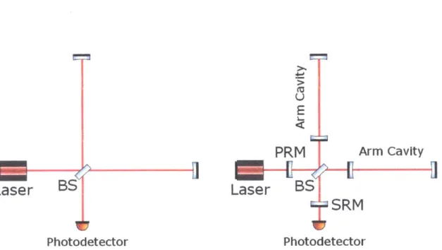
Quantum noise: ex-plained in the text. Seismic noise: caused by the local ground motion that the seismic isolation system could not suppress. Gravity Gradi-ents: caused by fluctuations in the local gravitational field, for exam-ple by atmospheric pressure change, seismic waves, or moving masses nearby. Suspension thermal noise: expansion and contraction of the suspension wires used to hold the mirrors due to thermodynamic flue-tuations. Coating Brownian noise: thermodynamic fluctuations in the mirror coatings. Coating Thermo-optic noise: changes in the refractive index of the coating material and the thermal expansion of the coating. caused by temperature fluctuations due to thermal dissipation in the coating. Substrate Brownian noise: thermodynamic fluctuations in the mirror substrates. Excess Gas: changes in the refractive index in the beam path due to resisual gases in the vacuum enclosure. . . . . 23

1-2 A schematic of 2 interferometer configurations. The left is a simple Michelson interferometer. The right is a dual recycled (signal and power recycled) Fabry-Perot Michelson interferometer configuration that Advanced LIGO uses. . . . . 24

1-3 Example sensitivities of QND interferometers compared to that of Ad-vanced LIGO. This plot is taken from 161. All three methods use low

1-4 The left shows a coherent vacuum state. The imiddle is a squeezed state in one quadrature., and the right is another squeezed state in the other quadrature. . . . . 27 2-1 A simplified schematic that shows how we can measure a mirror loss.

(a) is the most simple way to measure the loss, but often does not have enough accuracy. (b) shows the setup we use. With the acousto-optic modulator (AOM). we can control the input light frequency, or we can also cut off the light suddenly. . . . . 33 2-2 Schematic of an optical cavity for the loss measurement. . . . . 33 2-3 Ringdown measurement time series. . . . . 40 2-4 Simplified setup of the loss measurement. Cavity length d ~ 2m;

T, ~ 190ppm; T2 ~ lppm; Cavity finesse F ~ 30000. The cavity was

enclosed in a vacuum tank operating below 10-4 mbar and the optical table was floated to isolate the seismic vibrations. The cavity mirrors had ion-beam-sputtered coatings on super-polished, two-inch, fused-silica substrates with 10-5 scratch-dig surface quality and the RMS roughness <lA. All three photodiodes had a high enough band-width to measure the transients accurately without significant distortion in the tim e series. . . . . 42 2-5 A typical linewidth measurement and its fit. The residuals are offset

by -0.1 for clarity. Taken from [71. . . . . 43 2-6 A typical Doppler measurement and its fit. . . . . 44 2-7 A typical ringdown measurement and its fit. The blue points

corre-spond to the data and the green line correcorre-sponds to the fit. A small deviation at time t = 0 from the model is due to the finite bandwidth of the photodiodes. This plot is taken from 171 and modified. . . . . . 44 2-8 A comparison among loss measurement methods. The error bars from

each different method overlap and these measurements provide a con-sistent result. . . . . 45

2-9 dconfocal (or beam size) vs L,.t. At each beam size, we probed multiple beam positions on the mirrors. Each data point is a weighted average of multiple loss measurement techniques explained in Sec. 2.1. ... 46 2-10 dconfocal VS Lr/dconfocal for all the data points found in the literature.

The data points with a cross mark correspond to those that are more than 10 years old, and those with a circle are more recent data (the distinction was made because the loss seems to be lower for newer measurements due to improved technologies). There are scatters, but we can see a trend. The dashed line corresponds to Lrt/dconocal = (3.2m) ( )l0.63 _{to guide the eye. This plot is based on figure 10} of [P I. . . . . . . . . 47

3-1 A beam splitter model. . . . . 67 3-2 An example of Wigner funtion with r 1, = 0.5, > = 7r/8 in the Eq.

3.59. . . . . 74

3-3 An example of the ball-on-stick picture. The ball-on-stick picture can

contain the information about the squeezing angle and the squeezing

/ anti-squeezing levels. . . . . 75

3-4 All the diagrams are in the rotating frame of the carrier frequency wo. 76 3-5 On the left. the ball-on-stick pictures show a quasi-probably density

of the noise at a certain modulation frequency Q; this is an average of phasors between Q ~ (Q + dQ) and -Q ~ -(Q

+

dQ)., with respect

to the carrier frequency. The middle column shows how the sideband picture changes as the light goes through the squeezer and the quan-tum noise filter cavity. The quanquan-tum noise filter cavity modifies the amplitudes and phases of the phasors according to its response func-tion when the light is reflected. The phasors after the squeezer are drawn to be lined up so that it is easier to illustrate the effect of the quantum noise filter cavity, but they are actually rotating at their own modulation frequency Q. . . . . 78

3-6 A schematic of the hoinodyne detection setup. The 50-50 beam splitter

divides both the LO and the squeezed light into half and mixes the two beams, whose beat signals are individually detected by the two photodetectors. The signals are then subtracted from one another to get rid of the connon LO noises, and then the frequency components of the subtracted signal are measured by a spectrum analyzer to detect the quantum noise. . . . . 79

3-7 _{Schematic of an quantum noise filter cavity model. The mirror mIL is}

introduced to model the internal loss. . . . . 89

4-1 A block diagram of a system model with n devices. Each device is

represented by an operator O.. Typically our first device is a perfect frequency independent squeezer S. At each loss port, the beam power is lost by a factor of Li, and a coherent vacuum noise gets added. . . 96

4-2 A simplified schematic and model of the quantum noise filter cavity

experiment. Usq, is a transfer matrix for a lossless squeezer and the OPO loss is included in Lij. On the other hand, Uj, is not unitary and the loss factor /1 -- Lc is already built into U so we explicitly wrote out Lfc in the second loss port for clarity. . . . . 105

4-3 Schematic of a quantum noise filter cavity setup. The half wave plate is inserted to correct for a polarization change due to birefringence. . 112

4-4 Reflected power and phase, with and without a birefringence. The cavity parameters are the same as those in our experiment explained in Ch. 5. A linear birefringence of c = 50 prad is used. . . . . 116

4-5 Plot of the quadrature noise (ref. Eq. 3.24) as a function of the readout angle < (r is taken to be 1 for illustration). Suppose (a), (b) and (c) are some quadrature angles we want to measure. If there is no phase noise, the red line corresponds to the exact angle we want to measure. However, due to the fluctuation in our phase control system, what we actually measure is an averaged value of the angle shaded in pink. As you can see, squeezed quadrature (a) gets affected the most, compared to (b) or (c), because it is at the extremum and the slope is acute. . . 118

5-1 A simplified experimental setup for the audio-band frequency-dependent

squeezing. Taken from 121 and modified. . . . . 123

5-2 This plot shows how each MCMC chains evolved over steps. We can

see that after 100 steps, the chains are quite stable and the simulation is well "burnt-in". . . . . 128

5-3 The posterior distributions of frequency independent loss, phase noise, and nonlinear gain. . . . . 129

5-4 The frequency-dependent squeezing measurements. Each colored curve corresponds to a different quadrature angle measurement. The black dashed lines are the fit to the model explained in Sec. 5.3 and Chapter 4. The black solid line corresponds to the best possible sensitivity improvement if this was applied to an appropriate interferometer. The red ellipses below are the Wigner functions at each frequency. The colored axes on the ellipse correspond to each readout quadrature angle.130

6-1 A simplified schematic and model of the frequency-dependent

squeez-ing setup with the current interferometer configuration. . . . . 134

6-2 The quantum noise reduction using a 10dB squeezing and a 16 m long

quantum noise filter cavity. The parameters used are the same as in Fig. 6-3b. . . . . 136 6-3 Noise reduction due to frequency-dependent squeezing with a 16 m

List of Tables

5.1 Key experimental parameters. The asterisk indicates fit values. The fit and independent measurements were in agreement within their

un-certainties. . . . . 122

5.2 This table shows the priors used and the final fit values. N(pt, u) is a Gaussian distribution with a mean p and a standard deviation u.

U(a, b) is a uniform distribution between a and b. Each parameter is

Chapter

1

Introduction

1.1

Importance of Low Loss Cavities

This PhD work belongs to a series of efforts and experiments that aim to use a spe-cially tailored quantum state of light to improve high precision optical measurements. The centerpiece of this work is very high finesse (or, equivalently, low optical loss) op-tical cavities, which are often a criop-tical component in opop-tical precision measurements. For example, ultra-stable atomic clocks [9, 10, cavity quantum electrodynamics [11J, searches for vacuum magnetic birefringence [121 and quantum optomechanics [13, 14J all call for low loss cavities. In the applications for gravitational wave (GW) detec-tors, ultra low loss optical cavities play a significant role in circumventing the noise imposed by quantum vacuum fluctuations of the electromagnetic field. To surpass the quantum noise limit, we often have to manipulate light with specially engineered quantum correlations, but a quantum system is strongly susceptible to losses. As soon as the quantum system is exposed to the outside universe, the interaction would degrade the fragile quantum state and render it unusable even. Since a significant motivation of this work is to help improve the sensitivity of the laser interferometric

1.2

Gravitational Waves and Laser-Interferometeric

Detectors

1.2.1

Background

Just about 100 years ago, in 1916, Einstein used his new theory of General Relativity to predict the existence of GWs1l[15, 16]. According to his theory, massive objects moving in a spacetime would change the curvature of the spacetime around it, and the resulting ripple of spacetime curvature would propagate outward from the source as GWs. However, GW amplitudes are so tiny that any conceivable phenomena on the earth would not produce a detectable signal. For example, the GW amplitude from a source with quadrupole moment ,, (a system of two objects with mass M separated

by distance R that are rotating has quadrupole moment of M2_{R, for example) that}

is distance r away from us can be written as2_:

2G

hJIV = -ig ₁₁

From the factor G/c4_{, we already see that the effect is minuscule. Furthermore,}

just like all other waves, the GW amplitude decays as it travels, as required by the 'The idea of GWs was already explored by Laplace in 1805 [171, even though his analysis was wrong from the modern point of view.

2 This can be derived, up to a constant, by a simple argument of dimensional analysis using an analogy with electromagnetic (EM) waves. Just like the EM wave, the lowest order accelerating multipole dominates the wave production, but since there is no negative mass, GWs cannot have a dipole like EM waves, and it is an accelerating quadrupole that creates GWs. Also, just like the EM waves, GW amplitude decays as 1/r to conserve the radiated energy (for example, heuristically speaking, if we consider a sphere of radius r as our Gaussian surface with its surface area 47rr2 _,

the energy must fall as 1/r2 to conserve the energy, so the amplitude goes down as 1/r). Therefore, we guess that the GW amplitude takes a form:

h ~(1.2)

where I is the quadrupole moment of the system. Now since we are dealing with General Relativity, we use c and G to make the right-hand side into the same dimension as the left-hand side, and we get:

GI

h ~J -G (1.3)

rc

conservation of radiated energy. Therefore, by the time a GW reaches us from a distant source, it is extremely small and hard to detect. On the other hand, the information a GW may carry are highly attractive. From Eq. 1.2, we see that strong GW sources must have a large accelerating gravitational quadrupole, that is, they must be very heavy and moving very fast. In other words, the best GW sources are some of the most violent and interesting phenomena in the universe. For example, GW source candidates for the ground-based GW detectors include neutron star/blackhole binary collisions, supernova explosions, pulsars and the Big Bang itself

[18J. Not only are these interesting astrophysically, but these phenomena also provide

a strongly curved spacetime on which we can test fundamental laws of physics encoded in General Relativity. The fact that GWs interact very weakly with matter, which is painful from the detection point of view, can be a benefit because GWs can convey source information directly, without being interrupted or affected by any obstacles that lie between the source and us.

Given the anticipation that GW astronomy could greatly improve our understand-ing of the universe, there have been many attempts to detect GWs. Even though no direct detection of GWs has been reported yet, there is indirect evidence that GWs do exist

[191;

Weisberg and Hulse showed that the energy decay of a binary pulsar system inferred from its orbital time is in remarkable agreement of that of the GW emission predicted by General Relativity. Experimentally, the leading technology to directly detect GWs on the earth is based on the laser interferometry. Already in the 1960's, Gertsenshtein and Pustovoit proposed to use laser interferometry for the GW detection. Weiss at MIT carried out the first realistic analysis of the technique independently [201. As a GW passes by, it stretches and shrinks the distance between two freely falling objects, like suspended mirrors, by an amount proportional to the distance between the objects, AL = hL, along a fixed axis. So the basic idea of the laser interferometer is to measure a length difference change between two axes. Laser interferometry has an advantage over other techniques

[21,

221 in that it can have broadband sensitivity.

op-erating or under construction. There are two detectors in the United States called Advanced LIGO (Laser Interferometric Gravitational-wave Observatory), which cur-rently have the highest sensitivity and are taking data [5]. There is also Advanced VIRGO in Italy [231, and KAGRA in Japan 1241, that are being built and are ex-pected to have sensitivities comparable to that of Advanced LIGO. The sensitivity of Advanced LIGO is now reaching the level that we should be able to detect GWs soon if our current estimate of the sources is correct.

1.2.2

Noises due to Quantized Light

The GW amplitude is characterized by a quantity called the strain h, which is defined as h = AL/L, where AL is a fractional length change induced over a proper length L.

There are various noise sources that limit the strain sensitivity of GW detectors, and each noise source has a different frequency dependence. As we can see in Fig. 1-1, which is what we expect to have when the Advanced LIGO detectors are operating at their design sensitivity, the quantum noise is going to be a major sensitivity limit in most of the detection band. Therefore, even though there are many contributing noise sources (which are explained in the caption of Fig. 1-1), we are going to focus on the quantum noise in this work.

To see how this quantum noise arises, let us consider a simple Michelson inter-ferometer for a moment (the left panel of Fig. 1-2). According to the quantum theory, the photon number of a coherent beam has a inherent randomness, which is characterized by the Poisson distribution, due to photon number counting statistics

[251. Therefore, the photon number has an uncertainty of V(~N), where (N) is the

expected number of photons for a beam with a power P. This fluctuation in the photon number can have two different consequences for the GW detection. In this section, we carry out a heuristic calculation to analyze these two effects. A more rigorous treatment can be found in [261.

One effect is called the "shot noise", and it comes from our inability to measure the phase difference between two arms due to the photon number fluctuations. At the output of the interferometer, the photodetector measures the photon number per

-(i .1 t1

10C

Figure 1-1: The noise budget for the nominal mode (high power and broadband) of operation of Advanced LIGO (taken from

154).

Quantum noise: explained in the text. Seismic noise: caused by the local ground motion that the seismic isolation system could not suppress. Gravity Gradients: caused by fluctuations in the local gravitational field, for example by atmospheric pressure change, seismic waves, or moving masses nearby. Suspension thermal noise: expansion and contraction of the suspension wires used to hold the mirrors due to thermodynamic fluctuations. Coat-ing Brownian noise: thermodynamic fluctuations in the mirror coatCoat-ings. CoatCoat-ing Thermo-optic noise: changes in the refractive index of the coating material and the thermal expansion of the coating, caused by temperature fluctuations due to thermal dissipation in the coating. Substrate Brownian noise: thermodynamic fluctuations in the mirror substrates. Excess Gas: changes in the refractive index in the beam path due to resisual gases in the vacuum enclosure.

time. So we set up our device such that a phase difference between the two arms caused by mirror displacements appear in the photon number. But since the photon number fluctuates regardless of the differential phase, we cannot distinguish a signal from the random fluctuation. Because the randomness follows the Poisson statistics,

'U E PRM Arm Cavity

Laser

BTS

SRIM

Photodetector

Laser

oott

Photodetector

Figure 1-2: A schematic of 2 interferometer configurations. The left is a simple Michelson interferometer. The right is a dual recycled (signal and power recycled) Fabry-Perot Michelson interferometer configuration that Advanced LIGO uses.

the shot noise scales3as ( d(N) _dt ._.N1 Noting that

d(N) _ (P)

dt hw

we have the shot noise in a form:

- Lo 1 1

hshot (Q) = L ~

--L L ]

(1.4)

(1.5)

This noise dominates at frequencies above - 100Hz for the GW detectors.

The other effect is called the "radiation pressure noise". Because each photon has a momentum hk, the laser beam exerts a force on the mirrors as it gets reflected. Therefore, changes in the photon number flux can move the mirrors due to the pressure change, which directly competes with the GW effects on the mirrors. Note that, using Newton's Second Law, the force fluctuation in the frequency domain due to the photon

I One way to think about this is to consider each photon as an individual probe, and since our measurement is an average of n photon probes, where n is the average number of photons we detect during a detection time At, the uncertainty scales as fi/n = 1/n.

number fluctuation can be written as:

A Frad = MQ2A Lrad

[d(N)_ P

= 2hk dt - 2hk (1.6)

Thus, the noise due to the radiation pressure fluctuation becomes:

ALrad(Q)

V(1

hrad(Q)= L MQ2L _(1.7)

This noise dominates at frequencies below - 100Hz for the GW detectors. Now the total quantum noise is:

= hhot(Q) + h2ad(f ) (1.8)

Since the shot noise scales as 1/vip and the radiation pressure noise scales as

v7P,

there is an optimal power to minimize the quantum noise at a fixed frequency, and we call that minimum noise the standard quantum limit (SQL). This is a direct consequence from the quantum property of light, and as long as we use a classical state of light, we cannot beat this sensitivity limit. Even though we used a simple Michelson interferometer for this illustration, the shot noise and the radiation pressure noise also limit the sensitivity of the Advanced detector configuration (which is shown on the right panel of Fig. 1-2).

1.2.3

Gravitational Wave Detectors Beyond Quantum Limit

There are several techniques that can be used to circumvent the SQL, and such interferometers that can beat the SQL are called quantum non-demolition (QND) interferometers. These include a variational-output interferometer, which introduces optical cavities at the output to enable frequency-dependent homodyne detection

1271,

speed meters, which radically modify the optical topology design to measure the speed of the test masses instead of the displacement [28, 29, 301 (see Fig.

1-3). For any QND interferometer proposed, though, optical loss severely constrains 10--10 10 24 10

10~

Frequency [Hzj

Figure 1-3: Example sensitivities of QND interferometers compared to that of Ad-vanced LIGO. This plot is taken from

[6].

All three methods use low loss cavities.

their performance, so the characterization of low loss cavities is essential if we are to overcome the quantum noise limit.

Currently, the most mature and promising technique to go beyond the SQL is to use a squeezed state. A squeezed state of light is a quantum state whose uncertainty in one of the quadratures is reduced compared to that of a coherent vacuum state (see Fig. 1-4; a more detailed explanation is given in Ch.3). Caves first proposed to inject a squeezed state from the dark port of an, interferometer to reduce the shot noise [31]. This has already been demonstrated at the LIGO Hanford detector

1321, as well as at the GE0600 detector [33]. A frequency-independent vacuum state squeezed in the phase quadrature was injected into the interferometer from the dark

-Adv LIG(O

- -Sueezin Filer Caviiy

-Variationad Readout

-4 km Speedmneter

... .. . . .. ... I ( i

Figure 1-4: The left shows a coherent vacuum state. The middle is a squeezed state in one quadrature, and the right is another squeezed state in the other quadrature.

port, and it successfully improved the sensitivity in the frequencies where the shot noise dominated. In their demonstrations, technical noises such as thermal or seismic noises were covering the radiation pressure noise in the low frequencies.

For the Advanced LIGO era, due to the high input power and the reductions of classical noises, we expect that both low and high frequency band will soon be limited

by the quantum noises, as shown in Fig. 1-1. A complication is that the shot noise,

which dominates at the high frequencies, is caused by the phase quadrature noise, and the radiation pressure noise, which dominates at the low frequencies, is caused

by the amplitude quadrature noise. Therefore, to achieve a sensitivity improvement

over the full detection band, we need to manipulate the squeezed state as a function of frequency, so that the squeezed quadrature matches the frequency response of the interferometer. One way to realize this frequency-dependent squeezing is to reflect a frequency-independent squeezing off a Fabry-Perot cavity called "quantum noise filter cavity". In this thesis, we explored a low loss cavity that can be used as a quantum noise filter cavity, and demonstrated the frequency-dependent squeezing in the audio-band frequency.

1.3

Structure of the Thesis

This thesis has the following structure.

importance of low loss cavities, and review the current status of squeezing applications in the GW detectors. We especially argue that for almost any scheme that tries to circumvent the quantum noise limit, minimizing loss in optical cavities is critical.

Ch.2 is based on the published paper Il, where we measured the loss of state-of-the-art mirrors. For a fixed storage time, we need either a low loss or a long cavity. Therefore, loss is a key parameter in designing quantum optical cavities, and it determines how long a cavity should be for a particular application. We introduce multiple techniques (the linewidth, Doppler, and ringdown measurement) that can be used to measure the mirror loss with a very high accuracy. What is new from the paper is that (i) a simpler analytical expression for the ringdown loss measurement is derived, (ii) a closed form formula of the Doppler loss measurement is derived, and (iii) some justification is given to extrapolate our measurement results to a system with a different scale. Based on this loss measurement, we conclude that a 16 meter quantum noise filter cavity is long enough for Advanced LIGO detectors. This result is significant because a 16 meter cavity fits into the current LIGO facilities without any modifications on the vacuum enclosure (which is quite expensive and time-consuming).

Ch.3 reviews a general quantum optics theory that we use in our experiment.

Compared to the previous squeezing theses in the GW community, the emphasis is on the frequency dependence, and the formalism is recast to deal with continuous frequency.

Ch.4 is based on the published paper [3]. Using the theory developed in Ch.3, we construct a model to simulate our frequency-dependent squeezing measurement, including technical noise source contributions. We especially focus on the frequency-dependent degradation mechanisms, which are new to the experiment. This model is critical in designing a realistic filter cavity for Advanced LIGO.

Ch.5 is based on the submitted paper

141,

and explains the experiment of frequency-dependent squeezing in the audio-band frequency. In this experiment, for the first time, we demonstrated the frequency-dependent squeezing in the audio-band, whose technique can be applicable and scalable to GW detectors. We apply the model

de-veloped in Ch.4 to the result, and we conclude that this technique can be an early upgrade for Advanced LIGO to overcome the quantum noise limited sensitivity.

Finally, Ch.6 summarizes the thesis, and extrapolate our results and model to the Advanced LIGO case. We also discuss the current limiting factors of this technique and where we need to improve.

To provide the backgrounds and have a complete story, some materials presented in this thesis overlap with the previous works and theses. For those parts, I tried to offer an intuitive explanation or a different perspective, and referred to the previous works for more quantitative analysis and formulas. For the parts that require new treatments because of the frequency dependence, more detailed mathematical analysis is given.

Chapter 2

Cavity Loss Measurements

As we saw in Ch. 1, the loss in optical cavities plays an important role for many high precision measurements. Especially for -high finesse cavities, mirror losses can be a limiting factor for such measurements. Therefore, analyzing and developing a theory for cavity loss is critical in designing optical precision measurement. However, loss measurements are difficult because of their high accuracy requirement, typically of an order of one part in million (-ppm). Moreover, in some cases, we would like to know the loss as a function of beam size, so that we can extrapolate the result of loss measurements to a different scale and to various applications. For example, we would like to use a tabletop loss measurement to infer the loss expected in the GW detector applications, which is a much larger system with a different beam size. In this section, we first explore various methods to achieve a high precision measurement, show an experiment that implemented the methods to measure cavity loss, and finally, develop a theory to extrapolate the cavity loss to a system with a different beam size. The first two sections are based on

[71.

2.1

Loss Measurement Methods

We would like to measure the fraction of photons that get lost inside of an optical cavity. Since we place our cavity in a vacuum enclosure, the main sources of cavity loss come from the mirrors, such as absorption and scattering. The absorption loss

tends to be low for a kind of coating and substrate we use, and it is typically under

lppm

[341.

The scattering loss, which tends to dominate, comes from the aberration and point defects of the mirror surfaces. For a small beam size, we can usually avoid point defects by moving the beam position around on the mirror (the density of point defects on the Advanced LIGO mirrors, for example, is typically on the order of 1 per

5 mm2 _{[34]), but this cannot be done for a bigger beam sizes. In any case, we do not}

make a distinction among different loss mechanisms, but measure the combined loss that occurs inside of the cavity.

There are various ways to measure a mirror loss, but many of which do not pro-vide enough accuracy. For example, a simplest loss measurement we might think of is to measure the incident, transmitted and reflected power of a mirror as in Fig. 2-1a. Then the difference between the incident and the (transmitted + reflected) power would give us the mirror loss. However, since the loss we want to measure is very small, a slight calibration error of the three photodiodes can fail the accuracy requirement. A better way is to set up a cavity (see Fig. 2-1b). This is a natural choice because we often worry the most about the loss in a cavity, where a reso-nance can amplify the effect of the loss. It is relatively easy to measure the (loss + transmittivity) of cavity mirrors as we will see in Sec. 2.1.1 and 2.1.2, and by

sub-tracting transmittivity obtained from another independent measurement, we can infer the mirror loss. However, since we have to use a different setup for the transmission measurement, this is prone to a calibration error. For example, if we use different photodiodes for the two measurements, their calibrations need to be matched up to the same accuracy as our final measurement goal, which is quite challenging. What we need is a way to use a single setup with a single detector (i.e. one photodiode) to measure and separate the loss and transmittivity of the cavity mirrors. We show how we can accomplish this in Sec. 2.1.3.

In this section, we present three different ways to measure mirror losses. Because each method could have some systematic errors from a different origin, by comparing the various measurement results, we can gain confidence in our absolute value of the

Incident Diode Trans Diode Mirror Refl Diode (a) Lager Signal Generator Incident Diode

d

Trwi Dide

AOM _{Mi-ror 1 Minor 2}

Refl

Diode (b)

Figure 2-1: A simplified schematic that shows how we can measure a mirror loss. (a) is the most simple way to measure the loss, but often does not have enough accuracy.

(b) shows the setup we use. With the acousto-optic modulator (AOM), we can control

the input light frequency, or we can also cut off the light suddenly.

d

Lcav

Ti, Ri, Li

Mirror 2

T2, R2, L2

Figure 2-2: Schematic of an optical cavity for the loss measurement.

Throughout this section, we use the following notations. The reflectivity, trans-mittivity and loss of a mirror is referred to as Ri, T, Li respectively, where the subscript refers to mirror i = {1, 2} (see Fig. 2-2). Note that

Ri + T + Li =(2.1)

Lcav is a loss in between cavity mirrors, which is usually negligible but included here for generality. Each corresponding coefficient in amplitude is written in small letters,

L aser

Pi

-qPP-Pr--44-1

so that:

tj = V/T (2.2a)

ri = V/_1 - Ti - Li (2.2b)

tca 1 = "1 -Lcav (2.2c)

The cavity length is d and the wavenumber of light is k = A/27r, where A is the wavelength of light. We also define the incident power in the resonant mode' of the cavity as PO, the incident power that is in non-resonant modes as P (so that the total incident power is P = P + P1), the reflected power as Pr and the transmitted power as Pt. Now we define the cavity gain as:

1 2 G2 e (2.3) 1 - rir 2t av2ikd ___ 2 2, t2(2.4) 1 + rr tcav - 2r1r2t av cos (2kd)

(

-) ₂ (2.5) Ltot 1+ (Ltot /2

where we defined the total loss and the phase in a round trip as:

Lto0 T + L1 + T2 + L2 + 2Lcav (2.6)

6# [2kd]mod2r (2.7)

and assumed Tj, L, 6 < < 1 in the last line of Eq. 2.5. (In our experiment, T 200ppm, T2 - 1ppm, L, ~ L2 ~10ppm, 64 < 0.001, so keeping terms up to the

first order in them is a good approximation.) For a simpler notation, we write a

'A laser beam is assumed to be Gaussian and is decomposed in terms of orthogonal cavity modes [351.

normalized loss and phase as: -T1 Ti = _(2.8a) Ltot12 t2 = 2 (2.8b) Ltot /2 6 = (2.8c) Ltot12

Then the reflected power in steady state is:

Pr = POG -r1+ r2(t2 + r )tav e2ikd 2 + P1 (2.9)

~o l++ _{1 +} 2 +P1 (2.10)

6 2

and the transmitted power in steady state is:

Pt= PoGitit2tcavI2 (2.11)

SPO ₁ T1T2 (2.12)

+ 6#2

where we again used the approximation of T, Li, 60 < 1 in Eq. 2.10 and Eq. 2.12. As a check, when all the losses (L1, L2, Lcav) become zero, Pr + Pt becomes the total

input power (PO + P1).

2.1.1

Linewidth Measurement

One way to measure Let, of the cavity mirrors is by measuring the resonance linewidth of a cavity. From Eq. 2.12, if we slowly scan the input field frequency around a resonance, we get a Lorentzian peak of a form:

Pt = P0 T1T2. 2(2.13)

So by measureing the half width at half maximum of the peak (60q1wliNM) and using

Eq. 2.8c, we can derive Lt0t:

Ltot = 2

60 HWHM (2.14)

We can then subtract an independent measurement of transmission (T + T2) from

Lit, to infer the mirror loss.

2.1.2 Doppler Measurement

There is another way to measure Let~ using a dynamical response of the cavity, which we call the Doppler measurement [36, 37.

Let us define the roundtrip time of a cavity as Trt = 2d/c where c is the speed

of light in vacuum and d is the cavity length. Let us also define the round trip loss factor Pt as:

1 2

Prt rlr₂t~av - 2 (2.15)

in which we used the cavity finesse F, defined as:

.F = f FSR (2.16)

2

fHWHM

with the free spectral range of the cavity fFSR c/2d = 1/Tt and the half-width-half-maximum of the cavity fiiwiMl= fTSR6 0HWHA1/21r = fFSRLt/41r (see Eq. 2.14). Then, the field just inside of the input mirror in the cavity is:

Lt/TrtJ Ecav(t) = t1EO n

pte-i'(t'nrt) (2.17)

n=o

where a;, is the angular frequency at time t - nrrt. If the rate of change in frequency

in the rotating frame of w, Ec,, satisfies:

dEcay _{(t) ~ (Ecav(t + T-r) - Ecav (t))}

(2.18)

dt Trt

= (t1Eo + prte('~tt)rrtEcav - Ecav) (2.19)

Trt 1 - pis*(t-to)-rt t1 =- - Ecav + -- Eo (2.20) Trt Trt When S(t - to)'rrt << 1 (2.21)

(which we elaborate later), we can make an approximation:

1 - prt(iw*ttO ~ 1 - (1 - -)(1 + i6(t - tO)Trt) (2.22)

iF 7r

~ icZ(t - to)r,. (2.23)

= 1- ( i W / t to) (2.24)

W HW H MITs Tst

where we defined the cavity storage time Tst as:

st = -Trt (2.25)

We see that F/7r is the effective number of bounces that photons experience in the cavity, and we later found that Ti is the decay time constant of the cavity field without any input. Note that the condition 2.21 can be written as:

7r _{61o<< 1}

(2.26)

FWHWHM/Tst Tst

So for a high finesse cavity, this is a good approximation as long as the frequency change is modest compared to WHWHM/17t and the time series is cut off at a reasonable

time t. Therefore, if we define normalized unitless variables as: - I t = -(2.27a) T9 t o to (2.27b) Tst C 2 = 2(2.27c) WlHWIM/Tst

then Eq. 2.20 becomes:

dEc,(

d"" = - (1 - iF/(i- o)) Ecav + t1 _{E 2.28)}

Solving the differential equation gives:

Ecav(i) - e-(T-)eif f-) 2P/2 [e-e-io 2 V/2Ecav (0) (2.29)

. i-r -i20 ( + i(i -t~og (1+ i)i+ (f - j)7 a

+ -e z/2 erf- erf .

))

tii -E

22 2v= 2/ Trt

where erf is the error function 2. Noting that:

Ptrans = |t2Ecav|2 (2.30a)

p 2 + t2 ti 2

Pref - 1 -E0 + -Ecav (2.30b)

we can measure the transmitted/reflected power of the cavity while we change the frequency at a fixed rate3_{(i.e. W is some known constant), and fit the time series to}

extract the parameters such as Tt. Once we know rst, we can derive the loss Let,

(see Eq. 2.16 and 2.25). Again we have to subtract an independent measurement of the transmission (T1 + T2) from Let, to infer the mirror loss.

2_{This is a different expression than that used in the paper [71,}

but is a better approximation for a high finesse cavity because it is computationally lighter and captures the wiggling feature before a resonance.

3

We focused on the input frequency sweep because that is what we do in our experiment, but alternatively, we can also sweep the cavity length.

2.1.3

Ringdown Measurement

The above two methods can measure Lt,0 , but cannot distinguish the transmittivity

and the mirror loss. But by combining the information of a static and dynamic response of the cavity, we can distinguish and measure the pure loss of the mirrors.

Suppose we start from a steady state of a resonance cavity, and then we cut off the input field abruptly. Then, in the rotating frame of w, the cavity field just inside of the input mirror satisfies:

dE 1

dEcay ~ (Ecav(t + Trt) - Ecav(t)) _(2.31)

dt Trt 1 = (prtEcav -Ecav) (2.32) Trt Ec -Prt _(2.33) Trt = Ecay (2.34) 7-st

where we assumed that

mT

>> rt and used Eq. 2.15 and 2.25. Solving the differential

equation,

Ecav(t) = Ecav(0)e~/T" (2.35)

so using Eq. 2.10 and 2.12, the reflected light has the power:

1O( - t )1 + 6 2 P

Pr(t) + 6 2 _(2.36)

2

PO I - e-2/rt t > 0

where in the second line (t > 0), the form of the equation looks quite different from the first line (t < 0) because there is no promptly reflected light that interferes with

M2

0

I

Mn

3

I-Time Constant:

>1/mi

t0 =0

Time

Figure 2-3: Ringdown measurement time series.

the light from the cavity. Similarly for the transmitted light,

Pr()

={

P0 T1T2 1 + 6q 2 ~O ~ e T1T2 -2_t/Tst 1

+-

6<$2 (2.37) t > 0

Now for the reflected signal on the resonance, the equation reduces to:

Po (-T) +P1 t < 0 POT₁ e2-2t/,r t > 0

This time series is plotted on Fig. 2-3.

(2.38)

0

Now we measure, 2 7n, = ---T.st M 2 = 0 1 2 (2.39) m3 = Po 1 - Ti + Pi (2 M 4 Po+ P1

We get M1, M2 and m3 from the ringdown time series (see Fig. 2-3) and we measure

the power at an off-resonant frequency to get M4. From these measurements, we can

derive (Po, P1, t 1, rts). Recall that:

T, = Tr/ (2.40a)

Ltot / 2

ti = T/ (2.40b)

Ltot / 2

with Lit~ = T + L1 + T2+L2+ 2Lca. From Eq. 2.40a, we can calculate Ltot (we know

Trt by measuring the FSR of the cavity). We can assume there is no intra-cavity loss,

i.e. 2_{Lca, = 0, because the cavity is empty and placed in a vacuum enclosure. Now}

if we make one more assumption, for example the cavity is symmetrical (T = T2) or

the cavity is highly over-coupled (T2 = 0), then we can derive L, + L2, which is the

quantity we are after. (Alternatively, we can swap the input and output mirrors and repeat the experiment to avoid making this additional assumption.)

2.2

Experimental Setup and Measurement Results

This section explains the actual experiment that measured loss of super-polished mirrors with an ion-beam sputtered coating (Ref.

[7).

To minimize the systematic errors, we set up an experiment that can perform all three loss measurement methods explained in Sec. 2.1. Another feature of this experiment is that the cavity is very close to be concentric [351, so that we can explore various beam sizes on the mirrors and their effects on the loss by slightly adjusting the cavity length. By changing the

Refl

Diode

N", d

Laser SHG EOM PBS k/4 Mirror 2 Mirror 1

T rns _Refl

AOM Diode Diode

Incident

Signal Diode

Generator

Figure 2-4: Simplified setup of the loss measurement. Cavity length d ~ 2i; T, ~ 190ppm; T2 ~ 1ppm; Cavity finesse F - 30000. The cavity was enclosed in a vacuum

tank operating below 10-' mbar and the optical table was floated to isolate the seismic vibrations. The cavity mirrors had ion-beam-sputtered coatings on super-polished, two-inch, fused-silica substrates with 10-5 scratch-dig surface quality and the RMS roughness <IA. All three photodiodes had a high enough band-width to measure the transients accurately without significant distortion in the time series.

cavity length by 1cm or so, we could change the beam size from ~ 1mm to ~ 3mm. Since one of our goals was to extrapolate this loss measurement result to a length scale of the Advanced LIGO quantum noise filter cavity', the ability to measure the loss as a function of beam size was critical.

A simplified schematic of the experimental setup is shown on Fig. 2-4. Using

the frequency-doubled green light that shares the same light source as the red probe light, we locked the laser frequency to the cavity length via the PDH technique

[381

with about 40kHz bandwidth. We used the AOM to map out the resonant peak frequencies, which allowed us to calculate the FSR, cavity length, beam size, g-factor etc. of the cavity

1351.

Then again using the AOM, we can adiabatically change the frequency of the probe light to measure the linewidth, change the frequency rapidly (on the order of fHWHM/Tot) to perform the Doppler measurement, or cut off the

probe light abruptly to conduct the ringdown measurement. A typical measurement for each method is shown in Fig. 2-5 (linewidth), 2-6 (Doppler) and 2-7 (ringdown).

4_{A priori, we do not know how long the Advanced LIGO cavity should be. It could be a kilometer}

* Data Fit * Residuals 0.8 0.6- S0.4- 0.2-5 -10 -5 0 5 10 15 Frequency [kHz]

Figure 2-5: A typical linewidth measurement and its fit. The residuals are offset by

-0.1 for clarity. Taken from

11.

As you can see in Fig. 2-8, all the measurement methods give a consistent result when the error bars are taken into account. Following the formalism outlined in Sec. 2.1 and using an independent measurement of the input transmission T by a group at Caltech (which agrees with our ringdown measurements of T1; see [391) , we derived

the cavity mirror loss. We combined the results from each method by weighing the uncertainty to obtain the final loss value.

We repeated each measurement set with different beam sizes on the cavity mir-rors. For the GW detectors with a specific frequency response (which depends on its arm length, input power, mass of mirrors etc.), the storage time required for an optimal quantum noise filter cavity is already fixed. The total optical loss on a cavity resonance (where the loss is maximum) is:

total loss - (number of round trips) x (loss per round trip) T~ t -t L Lrt (2.41)

Trt 2 d

where we defined the round trip loss Lrt = Lt - T (i.e. the optical loss besides the input coupler transmission). Therefore, if we want to know the maximum loss

0.40 0.35 0.30 0.25 0.20 0.15 E 0.10 0.05 0.00 0 5 4 3 2 1 01 0 - Data -- Fit 200 400 600 800 1000 Time [is]

Figure 2-6: A typical Doppler measurement and its fit.

Off-reson a ice

Las~er On~i Laser Off

I _

-1 0

Time+0.05 Isi

On-resonance

Laser On Laser Off

Sexp(-mit) m3 exp(-m t) -1 x -2 ( Time his _x

Figure 2-7: A typical ringdown measurement and its fit. The blue points correspond to the data and the green line corresponds to the fit. A small deviation at time I = 0 from the model is due to the finite bandwidth of the photodiodes. This plot is taken

44 800 1000 200 400 600 0) 0 V Ii) LI 0) ci) cz 3 .J 5 -2

WW4

I I

208- 207- 206-205- -204 $ 203 202

Figure 2-8: A comparison among loss measurement methods. The error bars from each different method overlap and these measurements provide a consistent result.

for a quantum noise filter cavity with a given storage time, an important quantity to

characterize is Lt/d. In other words, for a given storage time, we can either have

a longer cavity or low loss cavity, and the cavity loss determines the length of the

quantum noise filter cavity. If we assume that the loss stays the same for the same beam spot size, a natural cavity configuration of the quantum noise filter cavity is

confocal because the confocal configuration has the smallest beam size for a given

cavity length, with the relation 1351:

dconfocal = A (2.42)

where w is the beam spot size and A is the wavelength of the laser. Thus, if we

want to answer the question "what is the minimum length of the quantum noise filter

cavity required for a given GW detector (which fixes the required storage time) with a minimum squeezing level requirement (which fixes the maximum loss we can allow)",

the best way to characterize our loss measurement is dconfocal vs Lrt/dconocal. Since our loss measurement gives loss as a function of beam size, under our naive assumption

Equivalent confocal length [m]

7.56 9.57 11.81 14.29

1.4 1.6 1.8 2 2.2

Beam spot size [mm]

17.00 19.96 23.15

2.4 2.6 2.8

Figure 2-9: dconfocal (or beam size) vs Lrt. At each beam size, we probed multiple beam positions on the mirrors. Each data point is a weighted average of multiple loss measurement techniques explained in Sec. 2.1.

that the loss stays the same for the same beam spot size, we use Eq. 2.42 to represent our result in terms of the equivalent confocal length dconocaI.

Our measurements probed the range of dconfocal from ~ 5m to ~ 25m, which is shown in Fig. 2-9. As we can see, within this range, the variation of the loss values is not that prominent, and stays roughly at a constant around ~ 10ppm, which is consistent with the scattering loss measurements done on our mirrors [1011 41].

Rather, the variation over the beam positions on the mirrors is larger (roughly 7ppm variation for each beam size). Therefore, as we construct a quantum noise filter cavity, it is important to move the beam spot on the mirrors around and find a "sweet spot" where we can minimize the loss.

2.3

Extrapolation to Different g-factor Systems

Because we want to extrapolate our measurement result for a longer cavity case, it is important to know if the extrapolation is valid. On a larger length scale, we see

5.79 20 18 16 14 12 10 8 6 I - I I

it-II ii

[

I

ii .4 - Ii - i . I.

-103 102 101 E (n C" -10 1 10-2 10,2 X 10- 10q 101

Equivalent confocal length 102 ("i""2 At') [M] 0 PVLAS 14 0 Battestb 08 Isogai 13 0 lsogaQ1 Isogai 13 0 Isogai 13 0 al-LO 14 X Ueda96 X Sato 99 Sato 99 ) LHO 2k 03 LHO 4k 03 X Kimble 92 W* X 103

Figure 2-10: dconfocal vs Lrt/dconocal for all the data points found in the literature. The

data points with a cross mark correspond to those that are more than 10 years old, and those with a circle are more recent data (the distinction was made because the loss seems to be lower for newer measurements due to improved technologies). There are scatters, but we can see a trend. The dashed line corresponds to Lt/doufocal =

3.2pm 0-.63 to guide the eye. This plot is based on figure 10 of 181.

I 3

PM ) 1M )

a trend in dconfocal vs Lrt/dconocal, as shown in Fig. 2-1.0. Empirically, this trend roughly follows:

Lrt ~ 3.2 ppm dconfocal 0.37

( m ).3

(2.43)

as seen from the dashed line in Fig. 2-10.

2.3.1

Theory of Loss Scaling and Beam Size

Since there is some scattering in the data, we cannot theorize the mirror loss com-pletely, but the general trend seen in Fig. 2-10 can be explained by the simple model

. . . I I I I

0 a 1