An analysis of ICBM navigation using optical observations of existing space objects

(1)

An Analysis of ICBM Navigation Using Optical Observations

of Existing Space Objects

by

Weldon Barry Willhite

B.S. Mechanical Engineering, United States Naval Academy, 2002

SUBMITTED TO THE DEPARTMENT OF AERONAUTICS AND ASTRONAUTICS IN PARTIAL FULFILLMENT OF THE REQUIREMENTS FOR THE DEGREE OF

MASTER OF SCIENCE IN AERONAUTICS AND ASTRONAUTICS

AT THE

MASSACHUSETTS INSTITUTE OF TECHNOLOGY JUNE 2004

ARCHVE

MASSACHUSETS INSTTUTE.

OF TECHNOLOGY

MAR

2 2 2010

LIBRARIES

The author hereby grants to MIT permission to reproduce and to distribute publicly paper

and electronic copies of this document in whole or in part.

Signature of Author ...

Department of Aeronautics Ad Astronautics

/'

Y?,1j4,

2004 C ertified by ...

C ertified by ...

Richard E. Phillips, Ph.D. Principal Member of the Technical Staff The Charles Stark Draper Laboratory, Inc. Techpical Supervisor

... ...

Jo6A E. Keesee, Col, USAF (retired) Senior Lecturer, Department of Aeronautics and Astronautics Thesis Advisor

A ccepted by ... ...

Edward M. Greitzer, Ph.D.

H.N. Slater Professor of Aeronautics and Astronautics

(2)

(3)

An Analysis of ICBM Navigation Using Optical Observations

of Existing Space Objects

by

Weldon Barry Willhite

Submitted to the Department of Aeronautics and Astronautics on May 14, 2004, in partial fulfillment of the

requirements for the degree of

Master of Science in Aeronautics and Astronautics

Abstract

This thesis investigates the potential of a space-based navigation concept known as Skymark to improve upon the accuracy of inertially-guided intercontinental ballistic missiles (ICBMs). The concept is to use an optical tracker to take line-of-sight measurements to nearby space objects with known ephemerides to update the state knowledge of the onboard inertial navigation system. The set of existing space objects that would be potentially useful for this application are tabulated, and a simulation determines their availability from realistic trajectories. A follow-on navigation

simulation investigates the accuracy improvement potential in terms of Circular Error Probable at impact. Two scenarios are investigated, one in which the Skymark system is

an add-on aid-to-inertial-navigation for an existing missile system, and one in which the Skymark system is completely integrated with a new inertial navigation unit. A

sensitivity analysis is performed to determine how several performance factors affect Skymark accuracy. Finally, a brief discussion of some operational implementation issues is included.

Technical Supervisor: Richard E. Phillips Title: Principal Member of the Technical Staff The Charles Stark Draper Laboratory, Inc.

Thesis Advisor: John E. Keesee, Col, USAF (retired)

(4)

(5)

Acknowledgements

Working on this thesis has been an incredibly enriching experience, and so I am very thankful to the Charles Stark Draper Laboratory for providing the opportunity for me to perform this research and study at M.I.T. I would also like to thank the U.S. Air Force ICBM Systems Program Office and Northrup Grumman Mission Systems for sponsoring my work here at the Draper Laboratory.

I am especially indebted to Richard Phillips, my technical advisor, who was

always available to answer my multitude of questions and provide exceptional guidance every time I found myself at a standstill. I would also like to express my gratitude to several other members of the Draper staff who have been supporting me in this research endeavor: Jim Shearer, Mary Biren, Bill Robertson, Ron Proulx, and Roy Setterlund.

My deepest thanks also are due to Colonel John Keesee, USAF (retired), my

academic advisor. His brilliant ideas and expert advice helped to steer this research in the right direction and ensure the thoroughness of this study.

I would also like to thank my wife, Jennifer, who has supported me through this

entire process. Thank you so much for encouraging me and being interested in my thesis, it has made a mighty difference!

Above all, I am thankful to God, who gave me both the ability and the strength to complete this work. Without Him I can accomplish nothing. He is my inspiration, motivation and reason for being.

Since ICBM accuracy values are classified, I have made assumptions of current accuracies based on unconfirmed values identified in open source literature.

This thesis was prepared at The Charles Stark Draper Laboratory, Inc., under internal project number 88002, contract number SUB HP 10786M8S (SLIN 0034), sponsored by the United States Air Force ICBM Systems Program Office and Northrup Grumman Mission Systems.

Publication of this thesis does not constitute approval by Draper or the sponsoring agency of the findings or conclusions contained herein. It is published for the exchange and stimulation of ideas

(6)

(7)

List of Figures

2-1 Locations of Inactive Space Objects... 27

2-2 Locations of Potentially Useful Space Objects... 28

2-3 Number of Skymarks Available -5,000 nm North-Firing Trajectory ... 39

2-4 Number of Skymarks Available -5,000 nm Northwest-Firing Trajectory... 41

2-5 Number of Skymarks Available -5,000 nm Northeast-Firing Trajectory... 41

2-6 Number of Skymarks Available - 7.0 Limiting Magnitude ... 43

2-7 Number of Skymarks Available - 8.0 Limiting Magnitude ... 44

2-8 Effect of Limiting Magnitude on Availability - Summer ... 45

2-9 Effect of Limiting Magnitude on Availability - Winter... 46

2-10 Percent of Sightings Achievable by Considering Smaller Catalogs... 48

2-11 Satellite Availability Considering the Original Catalog of 709 Objects... 48

2-12 Satellite Availability for Catalogs with 300, 200, and 100 Objects ... 49

2-13 Satellite Availability vs. Catalog Size -Summer... 51

2-14 Satellite Availability vs. Catalog Size -W inter... 51

3-1 Number of Skymarks Available -5,000 nm North-Firing Trajectory ... ... 65

3-2 Impact CEP (m) -5,000 nm North-Firing Trajectory... 66

3-3 Impact CEP vs. Satellite Availability, Initial CEP 1005 m ... 67

3-4 Baseline Performance Distribution for Skymark as a New System ... 69

3-5 Skymark Performance Distribution for Current System with High Correlation ... 71

3-6 Skymark Performance Distribution for Current System with Medium Correlation 72 3-7 Skymark Performance Distribution for Current System with Low Correlation... 72

3-8 Satellite Availability vs. Skymark Performance - Medium Correlation ... 74

4-1 Skymark Performance vs. Optical Tracker Angle Measurement Uncertainty ... 79

(12)

4-3 Skymark Performance vs. Quality of Skymark Ephemeris Knowledge... 85

4-4 Skymark Performance vs. Space Object Catalog Size... 86

4-5 Cumulative CEP Probability Obtained by Improving Parameters Individually... 88

4-6 Accuracy Probabilities Achieved by Improving Combinations of Parameters ... 93

4-7 Approxim ate Trajectory Tim eline ... 96

4-8 Impact CEP Probability Due to Sighting Trajectory Location ... 97

(13)

List of Tables

2.1 Satellite Selection C riteria ... 26

2.2 Number of Potential Skymarks in Altitude/Inclination Ranges ... 29

2.3 Percent Availability Variation Based on Limiting Magnitude ... 44

2.4 Percent Availability Variation Based on Catalog Size ... 50

3.1 Three Levels of Space Object Ephemeris Knowledge Considered ... 61

(14)

(15)

Chapter 1 Introduction

1.1 Thesis Motivation

Inertial navigation systems (INS) are the primary guidance technology enabling our natioWs Intercontinental Ballistic Missile (ICBM) fleet. In a world where strategic systems cannot afford to rely on the presence of GPS, inertial navigation offers a fairly accurate stand-alone guidance alternative for strategic systems. Today, the instruments and sensors that comprise the inertial measurement unit (IMU) of an ICBM are very high precision instruments. However, even the best IMU has errors that grow over time, so that at impact, several thousand nautical miles and 20-30 minutes downrange, these errors may have grown to relatively significant levels. When using low yield or conventional warheads in particular, an accurate impact is imperative both for effectiveness and the minimization of collateral damage.

The goal is to find a robust, relatively inexpensive means of improving ICBM accuracy. There are several options. The addition of GPS has been considered, but its susceptibility to jamming has prevented its use in strategic systems. A second possibility, further improving the inertial instruments, would likely be an extremely expensive

(16)

undertaking, as these sensors are already very accurate and costly. Some other method for in-flight aid to inertial navigation is sought.

1.2 The Skymark Concept

One idea proposed by the Charles Stark Draper Laboratory in Cambridge, MA, is for an add-on camera and software to incorporate the results of star and satellite angles-only observations to update the position knowledge of the INS. The concept, referred to

as Skymark, is similar to the age-old method used by mariners to triangulate their position by taking line-of-sight measurements to specific landmarks. The Skymark idea uses an optical tracker to sight nearby space objects as landmarks in the sky, or

"skymarks" as they will be referred to in this thesis, in order to estimate position in an angles-only fashion via triangulation. The basic concept of operations is as follows. A pre-launch process determines which space objects should be sighted using optimized selection algorithms, and uploads their ephemerides and associated pointing directions to the onboard flight computer. In flight, the camera makes line-of-sight measurements to the scheduled skymarks, using the star background as a frame of reference to determine the camera pointing direction. The missile INS flight computer maintains a continuous state estimate. The angular difference between where the skymark was expected to be seen (computed from a priori missile and skymark state knowledge) and its measured location on the star camera focal plane is calculated and used to update the missile state via Kalman filter equations.

The terms optical tracker and star camera will be used interchangeably in this thesis. Also, the capitalized term "Skymark" will be used to refer to the concept or the

(17)

onboard system, while the lower-case "skymark" will be used to refer to the space objects observed by the system.

1.3 Circular Error Probable and Impact Error Sources

Circular Error Probable (CEP) is defined as the radius of a circle inside which there is a 50% probability of impact. The CEP at impact will be used as the accuracy figure of merit in this study. Any system hoping to reduce the CEP of a missile must, by definition, reduce the sources of error that cause accuracy to degrade. The factors that affect the CEP of an ICBM can be divided into three main groups: navigation system errors, atmospheric conditions, and target location knowledge error. The CEP at impact can be understood as a root-sum-square of these factors. Thus, knowledge of which factors dominate the CEP and which ones can be reduced is required to assess CEP improvement. The assumption of this paper is that the navigation system errors dominate the CEP equation. Furthermore, of the three categories listed, only navigation system errors are those easily improved upon by means of technology improvement. Therefore, the presumption of this paper is that an improvement in navigation accuracy maps

directly to CEP improvement. For this reason, atmospheric conditions and target location knowledge will not be accounted for in assessing CEP improvement.

The navigation system errors for land-launched ICBMs are the position, velocity and attitude knowledge uncertainties associated with the IMU instruments. The Skymark concept aims to reduce these errors by means of optical observations of stars and nearby space objects. Stellar sightings provide the camera with self-attitude knowledge accurate to the level of its angular resolution. If tracker attitude knowledge can be successfully

(18)

related to IMU attitude (which may not always be the case, as will be discussed in Chapter 3), the error in IMU attitude can also be reduced to a level concomitant with tracker measurement accuracy. This "attitude update" will cause an improvement in CEP consistent with the amount of correlation between IMU attitude and position/velocity knowledge. In fact, the Navy makes good use of this idea, as their Trident submarine-launched ballistic missile (SLBM) is guided by a stellar-inertial navigation system.

In general, however, position updates are much more effective at improving accuracy than attitude updates. Obtaining updated position and velocity estimates

through angles-only observations of multiple nearby space objects is the main idea of the Skymark concept. When sighting nearby space objects, the tracker again uses the stellar background to obtain accurate pointing direction knowledge. By triangulating line-of-sight measurements of multiple space objects, the IMU position knowledge errors can be reduced to levels consistent with how accurately the position of the space object at sighting is known and how accurately its location can be measured by the tracker. In summary, each sighting of the star background can be used to update attitude knowledge,

and multiple sightings of nearby space objects can be triangulated to update position knowledge. As will be seen in Chapter 2, having visible skymarks available along every

trajectory at every time, while desirable, may not be feasible. In these cases, however, the optical tracker will yield some measure of accuracy improvement by performing attitude updates via stellar observations, as will be seen in Chapters 3 and 4.

(19)

1.4 Thesis Objectives

The primary objective of this research is to determine the potential accuracy improvement (in terms of impact CEP) offered by this concept. The scope of this thesis is to investigate the merits of the Skymark concept as applied to land-launched ICBMs. The analysis approach is to develop and run a series of realistic simulations that model various aspects of an operational Skymark system.

There are some obstacles, however, to performing this analysis in an absolute sense. For one, the exact performance of the navigation instruments in our nation's ICBMs is classified. For this reason, an error model simulating the position-velocity-attitude navigation error covariance matrix for the missile in flight must be created using unclassified information. Using general relationships as well as some parameterization, multiple cases will be investigated. The process of creating the IMU error models for these cases is described in detail in Chapter 3. A second difficulty arises from the fact that the accuracy with which the ephemerides of space objects may be known is also classified. Again, a parameterization is done, and various arbitrary accuracy levels are investigated. In this way, ranges of arbitrary capability levels will be studied for factors that are not public knowledge. Thirdly, some other parameters that affect impact accuracy are unknown because the Skymark system is still in the early phases of the research and development process. For example, the characteristics of the tracker, such as its measurement accuracy and sensitivity to the brightness of objects, are yet

undetermined. For these parameters, a range of feasible values (based on commercially available equipment) will be defined and investigated. Furthermore, operations aspects such as the amount of time necessary to maneuver the camera between observations,

(20)

calculate an updated position estimate, and perform any necessary post-update maneuvers are unknowns that must be mitigated through assumptions. A final unknown is the number of space objects necessary to compose a reasonably sized and valuable catalog for Skymark use. Determining this number is the primary subject of Chapter 2. Because there are so many variables in this study, a sensitivity analysis which determines the effect on the CEP of varying these parameters is a crucial part of the study. Presented in Chapter 4, this sensitivity analysis will help the decision maker determine which

elements will yield the most improvement for the least expenditure of money. The remainder of this thesis will be divided into the following sections.

Chapter 2 includes a methodology for defining a set of usable space objects for the Skymark system. The attributes of a suitable skymark are presented and applied to the set of all existing earth-orbiting objects in order to extract the subset of potentially useful satellites. Secondly, the development of a simulation to determine how frequently these satellites are visible from realistic ICBM trajectories is discussed. The results obtained from this skymark availability study are presented and will serve as the foundation for future chapters.

Chapter 3 continues with a description of an operational simulation for determining the potential accuracy improvement of the Skymark system. Two

implementation scenarios are investigated, one with the Skymark system as an add-on system to a current missile INS, and one with the Skymark system as a next-generation replacement navigation system including its own IMU. The goal of Chapter 3 is to determine the accuracy of the Skymark system if it were a present-day operational reality. To this end, values for the unknown parameters listed above are selected to represent

(21)

present-day capabilities (except for those parameters whose true values are classified, in which case an arbitrary value is assumed for unknown present-day capability).

Furthermore, the set of space objects used in this simulation are those selected by the availability study of Chapter 2. The CEP improvement afforded by Skymark for both scenarios is presented as a present-day benchmark.

Chapter 4 contains the sensitivity analysis. Because there are so many unknowns in this study, it is crucial to understand how the variation of parameters affects system performance. Specifically, since Skymark is not a current operational reality, it is interesting to investigate the performance effects of improving capability parameters to values that may be feasible in the near-future. Important trade offs are identified and discussed, and the sensitivity of the CEP to each variable in question is presented. Finally, a simplified cost analysis, comparing operations cost to development cost, is discussed and viable near-term solutions are postulated.

Chapter 5 contains a summary of conclusions, a discussion of some of the

significant issues surrounding the operational implementation of Skymark, and identifies areas meriting further study.

(22)

(23)

Chapter 2 Investigation of Satellite Availability

Initial Skymark studies at the C.S. Draper Laboratory, aimed at determining the validity of the concept, simulated Skymark measurements by using a computer-generated satellite constellation created for that purpose. Using this simulated space object catalog, these studies demonstrated that Skymark position updates have potential to significantly improve ICBM accuracy. This study aims to determine how well the Skymark system would perform if it were operational today and were thus to use a subset of existing space objects. To this end, the set of space objects that are actually in orbit around the Earth must be tabulated, and a simulation must be run to determine how frequently these

satellites are visible from realistic ICBM trajectories. Using the results of this availability study, one can begin to assemble an appropriate operational space object catalog.

2.1 Defining the Qualities of a Suitable "Skymark"

Although there are more than 5,000 objects larger than 10 cm in Low Earth orbit

[1], only a small percentage of them are appropriate or even necessary for Skymark use.

(24)

sufficient Skymark catalog will only require approximately 200-300 Earth-orbiting objects [2].

The first step in the approach to determining satellite availability is to determine the subset of current space objects that are potential candidates for the operational catalog. It is unnecessary to consider the vast majority of space objects that are

inappropriate for Skymark use by virtue of various reasons (e.g. orbit location). Thus, a set of constraints must be imposed on the database of all space objects in order to bound the feasible set. In order to determine these constraints, the attributes of a suitable

skymark must be defined.

As stated in the introduction, the accuracy of the Skymark system is dependent upon the accuracy of the predicted ephemeris and upon the accurate observation of the

skymark sighted. Therefore, for an object to be useful, it must have an accurately known ephemeris as well as good observability from realistic ICBM trajectories. These

requirements are the foundation for defining selection criteria for the Skymark catalog. The development of these criteria is explained in the following paragraphs.

Accurate ephemeris knowledge is crucial to Skymark because it has been shown in preliminary studies that CEP is proportional to ephemeris knowledge. Hence, satellites that are prone to maneuver should not be included in the operational catalog, and

therefore only inactive space objects will be considered. Secondly, objects classified in the satellite database as "debris" will not be included as their ephemerides are also very uncertain. Third, because of uncertainty due to atmospheric drag perturbation at low altitudes, it is sensible to consider only those satellites whose perigee altitude is greater

(25)

than about 800 km. This is a lower bound, and it is desirable to move this limit higher if possible.

Accurate tracker observations are equally important to the Kalman filter in the Skymark system. The accuracy with which the tracker can measure the line-of-sight direction to a nearby space object will dictate how accurately the observer location can be estimated. Because the tracker measurement uncertainty is angular, this accuracy will

decrease as the distance to the object being sighted increases. Thus, only objects whose orbits include points sufficiently close to realistic ICBM trajectories should be

considered. Current Skymark program accuracy goals combined with current

commercially available optical tracker capability give rise to a maximum apogee altitude criterion of approximately 2,000 km. Secondly, since the scope of this thesis is land-launched ICBMs, only north-firing trajectories from the Midwest United States are considered in this study. Therefore, all sightings will be taken over northerly latitudes, roughly between 50' and 90' latitude. Since it is desirable to minimize the distance to the skymark, only objects that traverse this region should be included in the Skymark catalog. Therefore, only those satellites whose inclinations are in the range of 5 0' - 1300

will be considered as potential candidates.

It is important to include a third requirement at this point. The second

requirement, measurement accuracy, assumed that the skymark appeared bright enough to be detected and observed by the optical tracker. However, the selection criteria that derived from this requirement, low altitudes and high inclinations, say nothing about whether the skymark will be visible to the tracker. Brightness, however, is a slightly more difficult requirement to work with. Each time any specific satellite is sighted, its

(26)

brightness is a complex function of the distance between the observer and itself, the sun-satellite-observer illumination angle, and the geometric and reflective properties unique to that satellite. Thus, a series of simulations must be run in order to determine which of the satellites that meet the first two requirements (accurate ephemeris and proximity to trajectories) are also frequently bright enough to be observed from realistic ICBM trajectories.

Current optical trackers have the capability to track objects as dim as about 6.0 instrument magnitude. Thus, the simulations will consider limiting magnitudes in the neighborhood of 6.0 when computing satellite availability.

The satellite selection criteria are summarized in Table 2.1. The criteria in this table that fall under the categories of ephemeris knowledge and measurement accuracy are straightforward and can be used to identify candidate skymarks. These potential space objects can then be tested for how well they meet the visibility requirement through

simulation.

Ephemeris Knowledge Measurement Accuracy Visibility " Listed in database as * Apogee altitude less than e Visible from simulated

"inactive" 2,000 km feasible trajectory with

* Not classified as "debris" * Inclination between 50' brightness less than 6.0

" Perigee altitude greater and 1300 magnitude (brighter) than 800 km

Table 2.1: Satellite Selection Criteria

2.2 Extracting the Set of Feasible Space Objects

The next step is to search through a current database of space objects for

candidates that meet the ephemeris knowledge and measurement accuracy criteria listed

(27)

above. The database used is the satellite database for Satellite Tool Kit, updated

December 30, 2003, and commercially available through Analytical Graphics, Inc@ [7].

A short program was written to sift through this database and identify candidates for the

Skymark catalog.

The preliminary filter searched the database for all entries classified as "inactive" but not classified as "debris," "coolant," or "metal object" (various database

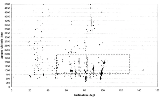
classifications for debris). Rocket bodies were not excluded from the search as they are large, reflective, and can be tracked with reasonable accuracy. A total of 3,069 space objects emerged. Their locations, plotted in terms of apogee altitude and inclination, are shown in Figure 2-1.

Locations of Inactive Space Objects (including Rocket Bodies but not including "debris") 5000 4750 4500 4250 4000 3750 3500 3250 3000 2750 2500 2250 2000 1750 1500 1250 1000 750 500 250 0-80 Inclination (deg) 120 140

Figure 2-1: Locations of Inactive Space Objects I.

*'

(28)

The outlined region indicates the approximate bounds of the altitude and

inclination limits discussed earlier (approximate because only apogee altitude is plotted and a small percentage of the skymarks depicted are somewhat eccentric). Thus, this region represents all criteria imposed by the ephemeris knowledge and measurement accuracy requirements. It may perhaps be expanded in the future as optical tracker technology improves. However, it does not appear that an expansion of this box will afford a significantly larger number of space objects (the box should not expand downwards because of drag uncertainty at lower altitudes). This region is blown up in Figure 2-2.

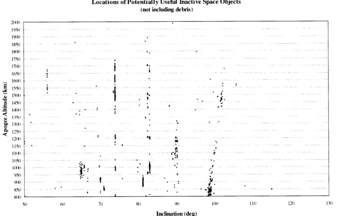
Locations of Potentially Useful Inactive Space Objects (not including debris)

2(XX) 1750 19(X) 145() 18(X) 1750 17(X) 1650 16(X) 15() 15W S13(XX) 1250 1150 )

IM).

95))0. 85) -8W) 50 6() 70 80 90 10W 110 120 130 Inclination (deg)

(29)

All potential skymarks, 1, 160 in total, are depicted in Figure 2-2. The task at

hand is to find an appropriate Skymark catalog among these 1,160 objects. Table 2.2 interprets the data depicted above.

Inclination Rancie Altitude Range 85-95 80-100 70-110 60-120 50-130 800-900 2 54 80 84 84 800-1000 5 190 234 298 298 800-1100 26 385 436 518 518 800-1200 55 418 479 562 564 800-1500 68 525 890 978 981 800-2000 68 548 1056 1145 1160

*Altitude Range is defined as the range that the space object always exists in

Table 2.2: Number of Potential Skymarks in Altitude/Inclination Ranges

This table shows the number of potential skymarks located in each altitude and inclination range of interest. The inclination range gets larger from left to right, and the altitude range increases from top to bottom. Thus, each entry in the table includes all the skymarks from entries above and to the left of itself in the table. Because lower altitudes and higher inclinations are more desirable (for measurement accuracy reasons), the goal is thus to find a useful skymark catalog that is as close to the upper left corner of this table as possible. Although it would also be desirable to increase the minimum altitude cutoff to 1000 km because of drag uncertainty in ephemeris predictions, a quick look at this graph and table will show that a significant number of potential skymarks exist in the

800 - 1000 km range, and thus this range is included in the study.

For the purposes of this availability study, all 1,160 potentially useful skymarks will be considered in the simulations described in the following sections.

(30)

2.3 Determining Satellite Availability via Simulation

In order to determine a potential satellite's usefulness to Skymark, a set of simulations must be run to determine how often it is visible from realistic ICBM trajectories. The methodology for developing these simulations is described in the following paragraphs.

2.3.1 Trajectory Assumptions

Obviously, one cannot expect to consider all trajectories for all times, and so a certain amount of discretization must be done without going to the point of losing

generality. This is accomplished via the following assumptions. First, it is assumed that all launches occur from a point in the Midwest United States that is in the vicinity of true ICBM launch locations. Secondly, it is assumed that every launch is a north-firing or near-north-firing launch. Third, given the approximate maximum range of current ICBMs (6,000 nautical miles) and considering areas of the Earth that could be potential targets (land mass), ranges between 4,000 and 6,000 nautical miles and launch azimuths within 400 of north (320' - 40') were chosen to bound the trajectory envelope for the

study. It is thus assumed that by taking into account 4,000, 5,000 and 6,000 nm trajectories on launch azimuths of 320', 00, and 40', the set of feasible trajectories is

spanned. These nine trajectories comprise both the limits and center of the feasible region, and it is thus assumed that investigating satellite availability over these nine trajectories will give a sufficiently accurate measure of skymark availability.

Next, the portion of the trajectory where observations can be taken, as well as the number of observations that may be taken in that window, must be defined. To do this, the operational functioning of the system must be taken into consideration. Between

(31)

engine cut-off and re-entry vehicle (RV) deployment, the system must have sufficient time for all scheduled observations, the calculation of an updated position estimate, and

any necessary corrective maneuvering in preparation for RV deployment. Because the tracker will likely have to be bolted down somehow, it is assumed that the entire bus will

have to maneuver between each sighting opportunity. Therefore, it is assumed that sightings will not be able to be any closer than approximately 2-3 minutes apart. Also, it is advantageous if the tracker can take multiple line-of-sight measurements to each skymark sighted as it crosses its field-of-view, allowing the tracker to better determine its position in space. The computational time necessary for post-processing the observation data to arrive at an updated position estimate is considered negligible. Finally, the time required for any necessary maneuvers prior to RV deployment is assumed to be

approximately 2-3 minutes. For the purposes of this availability study, it will be assumed that RV deployment may be delayed until the onboard resources of battery power and maneuvering fuel are depleted. This may not always be the case operationally, as will be discussed in Chapter 4. It is further assumed, based on indications from prior study, that onboard resources will be depleted around apogee. Therefore, the assumption in this chapter is that the time between engine cutoff and apogee, a span of 10-15 minutes depending on range to target, is the window for performing Skymark operations. Based on the time assumptions described above, it is assumed that there is enough time in this window for four equally spaced sighting opportunities. The time from cutoff to apogee will thus be divided by four, and the sighting opportunities will be defined as occurring at the beginning of each of these four time segments in order to allow time for maneuvering prior to RV deployment at apogee.

(32)

In order to calculate this portion of each trajectory, a Matlab routine is used to calculate the missile state at cutoff from the inputs of launch coordinates, target

coordinates, re-entry angle, and cutoff altitude. Next, a simple Keplerian Matlab routine is used to propagate the state from cutoff to apogee. The time from cutoff to apogee is divided by four, and the coordinates for each of the four "sighting locations" along each trajectory are calculated. To this point, 36 sighting locations (4 for each of the 9 trajectories) have been identified in earth-centered earth-fixed (ECEF) coordinates, and these 36 points are assumed to span the entire operational sighting envelope. Thus, the satellite availability simulation is a calculation of the number of potential skymarks that are visible from the sum of the four points on any given trajectory for all launch times.

2.3.2 Launch Time Assumptions

Nine discrete trajectories have been chosen; a set of discrete launch times for these trajectories must also be chosen. Because it is desired to capture all seasonal effects with respect to lighting conditions as well as satellite locations, an entire year must be simulated. It would be computationally impractical to consider a set of launches every minute for an entire year, and yet it is possible for a satellite to move in and out of view in such a small time period. Thus, a time interval for sampling must be chosen that will give accurate statistical results. The orbital period of the candidate space objects ranges from 100 to 120 minutes. The Nyquist sampling rule states that accurate results may be obtained by sampling at greater than 2.1 times the orbital frequency, or approximately 45 minutes. Because of computational constraints and the goal of obtaining the most

(33)

sampling satellite availability at 30-minute intervals for an entire year, accurate results may be obtained.

2.3.3 Catalog Propagation

Finally, a method of computing the location of each potential skymark at all times of interest is needed. Because the goal of this simulation is simply to determine

visibility, pinpoint accuracy is not required. However, a fair amount of accuracy is necessary, as an error on the order of tens of kilometers could affect the brightness that the simulation calculates. A single two-line element set (TLE), when propagated over long periods of time, becomes highly inaccurate, and thus not appropriate for this study. During previous Skymark efforts at the Draper Laboratory [2], a database was compiled consisting of unclassified two-line element sets for each day of the year 2003. The simulation will use this database to obtain ephemeris information that is at most 24 hours old, thereby avoiding significant satellite position errors. A program was written to extract the appropriate TLE data from this database, and write this data into a Matlab structural array. Thus, at the beginning of each day in the simulation, the appropriate part of the structure is accessed. As the day progresses, the ephemeris for each satellite is propagated forward to the time of interest using a separate Keplerian propagation routine with inputs of decimal Julian date and TLE epoch data.

2.3.4 Simulation Sequence of Events

The sequence of simulations is as follows. Beginning January 1", and for each day of 2003, consider missile launches at thirty minute time intervals. The first launch is at midnight local time on the day in question. For every launch time, consider each of the

(34)

nine trajectories. For each trajectory, consider in order each of the four stored sighting locations. Based on the launch time and the stored time interval to each of the sighting locations, the sighting time for each sighting opportunity is quickly calculated. The set of potential skymarks is then propagated to that time, and all satellites "in view" from the sighting location are tabulated. "In view" is defined as:

* The satellite is sunlit

* The observer is not looking directly into the sun to view the skymark (a 10-degree sun mask angle is defined)

e The earth does not eclipse the observer's view of the satellite

For each satellite in view, the simulation then runs a subroutine that computes the brightness of the satellite in question. This brightness calculation is somewhat more complicated and is described in the next section.

2.4 Calculating the Instrument Magnitude

The magnitude at which a skymark is "seen" by an optical tracker is a complex function of the distance between the observer and itself (R), the sun-satellite-observer illumination angle (ax), and the geometric and reflective properties unique to that satellite. The difficulties arise with this last aspect. Short of doing intensive research into every candidate space object to determine its properties of reflectivity, shape, and cross-sectional area, one can merely estimate these properties in a general sense (e.g. by assuming an average reflectivity constant for all skymarks). However, amateur satellite observers have already done much of this work experimentally. In [6], for example, one can find a database including "intrinsic magnitudes" for many satellites. The intrinsic magnitude is defined as the visual magnitude viewed when the satellite is 1000 km from the observer and the satellite is 50% lit (the illumination angle is 900). Because

(35)

brightness also depends on the orientation of the satellite being observed (a random phenomenon for many of the objects investigated because they are inactive), this intrinsic

magnitude can be viewed as the expected value of the brightness at R = 1000 km and a= 900. This database, however, does not include intrinsic magnitude values for many of the 1160 potential skymarks. The decision was thus made to only consider those space

objects with available and consistent intrinsic magnitudes, a total of 709 of the original

1160 candidates.

Given the database of intrinsic magnitudes, it is relatively straightforward to extract the reflective and geometric properties of a specific satellite by isolating these properties in the equation for computing brightness. The equation used for calculating visual magnitude is as follows:

Mag = 5 * log10 (R) -(2.5 * log 10 (I) + 18.8) (2.1)

where: I = (780pr) (2.2)

3/T * sin(a) + (i - a) * cos(a)l

R = Range from observer to skymark

I = Illumination angle dependent intensity

p = Satellite reflectivity

a = Sun-satellite-observer illumination angle r = effective radius of satellite

If the satellite has reflectivity p , and effective radius r, the original equation, Mag =f(p,

r, R, a), can be manipulated into the formf(p, r) =f(Mag, R, a). Knowing the intrinsic

magnitude, and the range (1000 km) and solar angle (90') that it applies to, the value of the function of p and r, which encompasses both geometric and reflective characteristics, can be calculated and stored. This "p r" factor can then be used in the original form of

(36)

the equation to calculate magnitude for any range and illumination angle. In the

simulation, the range is known because the coordinates of the skymark and the observer at the time of sighting are known. Secondly, the illumination angle is calculated by a subroutine that computes a unit vector to the sun for any given time. Finally, Equations 2.1 and 2.2 are used to compute the expected visual magnitude of the skymark from the

inputs of range, illumination angle, and the previously computed "p r" factor for the space object in question.

The brightness calculated by this routine, however, is still not the desired number. The magnitude calculated is visual magnitude, but the tracker is sensitive to a different frequency band. Assuming the use of a silicon-based star tracker, such as the Ball Aerospace CT-633, the instrument magnitude should be approximately .4 magnitudes brighter than the visual magnitude calculated [4]. Secondly, the intrinsic magnitudes

assume that the satellites are being viewed from the Earth's surface, and thus account for atmospheric extinction. Assuming that atmospheric extinction causes brightness to degrade by approximately 0.2 magnitudes, this means that the same satellite viewed from outside the atmosphere will appear 0.2 magnitudes brighter under the same illumination conditions. To sum up, the equations used in the simulation are only valid to calculate the visual magnitude of an object as viewedfrom the suiface of the Earth. Therefore, to adjust the calculated brightness for Skymark purposes, 0.6 magnitude should be

subtracted (brighter) to obtain the instrument magnitude as viewed by the optical tracker at post-boost ICBM trajectory altitudes. In an effort to be conservative, this factor will be rounded to 0.5 magnitudes for use in the simulation.

(37)

2.5 Satellite Availability Tabulation

At each sighting location, the simulation determines which skymarks are "in view" and calculates their visual magnitudes. At this point a matrix is formed containing all pertinent sighting information, including the North American Aerospace Defense Command (NORAD) satellite number, brightness, range, and illumination angle for each of the satellites in view. This matrix is stored in 4-dimensional Matlab structural arrays with the dimensions being day number, time of day, trajectory number, and sighting location number.

Clearly, this simulation involves an extensive amount of computation, and in fact takes several days to run a simulation considering 9 trajectories at each of 48 launch times during each of 365 days, for a total of 157,680 launches. Furthermore, for each of these launches, the catalog of skymarks is propagated to a specific sighting time 4 times, and, at each of these times, every potential skymark in the catalog is checked for

availability. At each one of these 788,400 sighting opportunities, an N-by-5 summary matrix containing all valuable sighting information is stored. This storage amounts to approximately four gigabytes of data that will require further programs to analyze. It is certainly desirable to run this simulation end-to-end only once, ensuring that all

potentially relevant data is stored for later use.

2.6 Skymark Availability Results

Once all sighting information has been stored, it can be accessed in a number of ways to present valuable results. In particular, it is desired to understand the effects of seasonal variations, limiting magnitude, and catalog size on satellite availability.

(38)

Ultimately, satellite availability will affect the performance of the Skymark system, as will be seen in the results of the next chapter. The graphs presented in this section display the number of bright skymarks available along a given trajectory by time of day and time of year of launch. The graphs for different trajectories are very similar, and therefore all nine will not be included in this section, but only those necessary to convey the important information. Results for all of the trajectories are included in appendix A. The north-firing, 5,000 nm trajectory will be the main one used in displaying the results since this trajectory is in the middle of the envelope for this study. Also, 6.0 is used as the baseline instrument magnitude cutoff value, as it is representative of present-day optical tracker capability. Unless otherwise noted, all graphs in this section account for all 709 potentially useful space objects.

2.6.1 Variations Due to Launch Time

Launch time is an important factor causing variation in satellite availability. Both time of day and time of year affect the number of bright skymarks available. This is not a

surprising result, since lighting conditions are a key factor in satellite visibility. Figure

2-3 depicts the number of bright skymarks available from the north-firing, 5,000 nm

trajectory by time of day and time of year, with a limiting magnitude of 6.0. This figure can be seen as a flattened sphere, since both axes are time and thus wrap around on themselves. The areas of black indicate times when 4 or less bright skymarks are available along the entire trajectory. The gray areas are those times when there are between 5 and 20 visible skymarks along the trajectory. Finally, the white areas of the graph indicate times when more than 20 bright skymarks are available. The table accompanying the graph helps explain the data depicted.

(39)

Number of Available Skyrnarks -North-Firing 5000nm -6. 0 Limiting Magnitude 20:00 f-4 18:00 16:00 -14:00 30 1 12: 00 25 10:000 40 8:00 a 6:00 20 4:00 10 2.00 5 Midnight 50 100 150 200 250 300 350 Day of Year Number of Skymarks 1 5 20 50

Percent of Time at Least That Many Available 98.68% 93.23% 81.06% 25.98%

Figure 2-3: Number of Skymarks Available -5,000 nm North-Firing Trajectory

There are several key observations one can make from the figure and table above. First, the center of the black area is approximately midnight on the Winter Solstice. This result makes sense, as midnight on the winter solstice is the worst time of year for

lighting conditions for a north-firing launch from the northern hemisphere. For this launch time, the sun is on the opposite side of the earth from the missile for much of its trajectory. Even as the missile comes up over the North Pole, the sunlight is still concentrated in the southern hemisphere, and most of the space objects that are actually

sunlit and in-view are far away and have obtuse sun-satellite-observer illumination angles (they are back-lit). For this reason, all satellites in view appear very dim, and will not be seen by a tracker with a limiting instrument magnitude of 6.0. Therefore, unless a more sensitive tracker capable of viewing dimmer objects is used or the observation period is extended past apogee, Skymark performance may be adversely affected by launching in

(40)

the vicinity of midnight and the Winter Solstice. However, as discussed in the

introduction, performing stellar sightings in lieu of skymark sightings in this case will accomplish some measure of CEP improvement, the extent of which will be presented in the next Chapter.

A second phenomenon observed in Figure 2-3 is that, once the launch time exits the black region, the conditions very quickly become very favorable. Once the lighting conditions improve even slightly from the worst case, many bright skymarks appear. In fact, 81 % of the time there are in excess of 20 bright skymarks visible along the

trajectory, and 93% of the time there are at least 5 available. Furthermore, 26% of the time, under near-optimal lighting conditions there are in excess of 50 bright skymarks

available. These times of maximum availability surround the best case scenario of launching at noon on the Summer Solstice. Having so many bright objects available is

not a surprising result because a large catalog of 709 space objects is being considered. With appropriate lighting conditions, many skymarks become visible. The effect of

launch time on satellite availability can be further seen by looking at graphs for the trajectories with northwest (3200) and northeast (40') launch azimuths. Figures 2-4 and

2-5 show the analogous plots for the northwest and northeast firing trajectories,

(41)

Number of Available Skymarks -Northwest-Firing 5000nm -6.0 Limiting Magnitude 22:00 20:00 1:00 16:00 14:00 12:00 10:00 8:00 6:00 4:00 2:00 Midnight Day of Year Number of Skymarks 1 5 20 50

Percent of Time at Least That Many Available 94.34% 88.13% 72.27% 9.62%

Figure 2-4: Number of Skymarks Available -5,000 nm Northwest-Firing Trajectory

Number of Available Skymarks -Northeast-Firing 5000nm -6.0 Limiting Magnitude

22:00 20:00 ii 18:00 .I 16:00 14:00 12:00 10:00 8:00 6:00 4:00 2:00 Midnight 5 0 II I 1 1 I I 150 200 250 Day of Year Number of Skymarks 1 5 20 50

Percent of Time at Least That Many Available 93.96% 87.91% 71.51% 10.54%

Figure 2-5: Number of Skymarks Available -5,000 nm Northeast-Firing Trajectory

(42)

It is clear from these graphs that they exhibit the same seasonal behavior as the north-firing trajectory. However, their areas of minimal satellite availability are offset from the north-firing trajectory by a couple of hours on the time of day axis. This result is to be expected. For instance, if an ICBM were launched to the northeast a few hours before midnight, it would find itself over the time zones where it is approximately midnight during the sighting window. The converse is true for the west-firing

trajectories, and thus the worst time for firing to the west is a few hours after midnight on the Winter Solstice. Secondly, the black areas in the northeast and northwest trajectory graphs are slightly larger than the black area in the graph for the north-firing trajectory. The reason for this result is as follows. For a launch in the vicinity of midnight on the Winter Solstice, the north-firing trajectory heads over the North Pole directly into the sun, but the sun does not come into view until relatively late in its trajectory (it is concentrated on the southern hemisphere). For this reason, the missile does not come very close to sunlit space objects until it is well along in its trajectory, and since it is heading toward the sun, it is even later in the trajectory before these objects become

visible due to favorable illumination angles (while the missile is approaching sunlit objects, it cannot see them because they are back-lit). As time moves away from the Winter Solstice, a north-firing missile launched at midnight will find favorable lighting conditions earlier in its trajectory. Because it travels over the North Pole, satellite availability at local midnight reappears sooner after the Winter Solstice than for the northeast and northwest trajectories, which do not even go above 700 latitude.

In discussing seasonal effects pertaining to satellite availability, it is necessary to note that for different launch locations, the graphs in this section may look very different.

(43)

For instance, if the launch location were in the southern hemisphere, the worst-case scenario would be launching on the Summer Solstice. If the launch site were on the equator, the Equinoxes would be the best-case and both the Summer and Winter Solstices would be equally worst-case.

2.6.2 Limiting Magnitude Effects

The next question of interest is the effect of the tracker sensitivity on satellite availability. In particular, it is desired to understand the extent to which the holes in satellite availability could be decreased by using a tracker capable of sighting dimmer objects. Figures 2-6 and 2-7 depict the satellite availability for the 5,000 nm north-firing trajectory if the tracker is capable of viewing objects down to 7.0 and 8.0 magnitudes, respectively. Numb 22:00 20:00 18:00 16:00 14:00 d 12:00 10:00 8:00 6:00 4:00 2:00 Midninht

er of Available Skyrnarks -North-Firing 5000nm -7. 0 Limiting Magnitude

IU

.

U

50 100 150 200 250 300 350

Day of Year

Figure 2-6: Number of Skymarks Available - 7.0 Limiting Magnitude

ginih

(44)

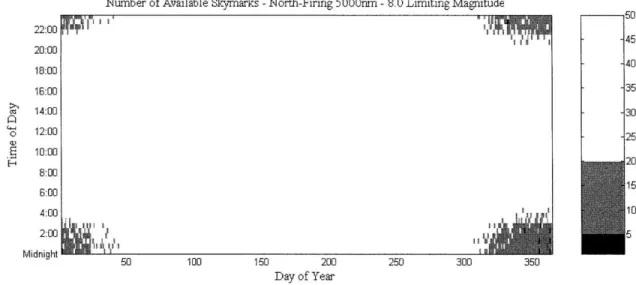
Number of Available Skymarks -North-Firing 5000nm -8.0 Limiting Magnitude 22:00 20:00 18:00 40 16:00 35 14:00 30 o 12:00 ₂₅ 6 10:00 20 8:00 6:00 15 4:00 10 2:00 5 Midnight 60 ₁₀₀ ₁₅₀ ₂₀₀ ₂₅₀ 300 350 Day of Year

Figure 2-7: Number of Skymarks Available - 8.0 Limiting Magnitude

Table 2.3 summarizes the effect of tracker sensitivity as depicted in Figures 2-6 and 2-7.

At Least Number of Skymarks Available 1 5 20 50

Tracker Limiting Instrument Magnitude

6.0 98.68% 93.23% 81.06% 25.98%

7.0 99.85% 97.43% 89.77% 78.49%

8.0 100% 99.93% 96.07% 88.56%

Table 2.3: Percent Availability Variation Based on Limiting Magnitude

These two figures show some very interesting results. First, with 7.0 as the limiting magnitude, 97.4% of the time the missile will see more than five visible

skymarks along this trajectory. This is an improvement over the 93.2% of the 6.0

limiting magnitude case for this trajectory. Furthermore, for the 8.0 magnitude case, this increases to 99.9%. In fact, for the 8.0 magnitude case, there is at least I visible skymark along the trajectory for every launch considered and greater than 50 bright skymarks almost 90% of the time. Other trajectories have similar results. For all nine trajectories

(45)

studied, a limiting magnitude of 8.0 guaranteed at least one bright skymark for 99% of launches, and at least five bright skymarks 95% of the time.

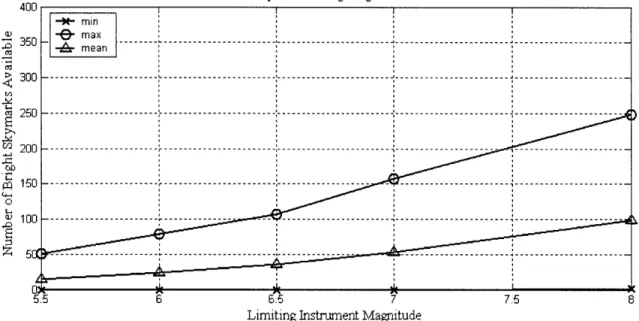
Figures 2-8 and 2-9 are summary graphs of the effect of tracker sensitivity on satellite availability for the summer and winter, respectively, for the north-firing 5,000nm trajectory. These two figures take into account all launches for the 30 days surrounding the summer and winter solstice. The data points plotted are the minimum, maximum, and mean number of bright skymarks available for the time of year corresponding to the graph.

Availability vs. Limiting Magnitude -Summer

400 -44 min 7350 -. men 350 --- 250---- --- ------ --- - - - -- - - --4 0 -4 5.5 6 6.5 7 7.5 8

Limiting Instrument Magnitude

(46)

Availability vs. Limiting Magnitude -Winter 400 -M- min Lmi mean 0

Figure 2-9: Effect of Limiting Magnitude on Availability -- Winter

Figures 2-8 and 2-9 demonstrate the extent to which availability increases with tracker sensitivity. For example, in Figure 2-9 (wintertime) it is observed that with a tracker capable of viewing objects at magnitude 6.0 and brighter, there are, on average, 25 bright skymarks available along the trajectory. An increase in tracker sensitivity to

view objects as dim as 8.0 magnitudes causes the average availability to increase to 100 bright skymarks, a rather significant increase. Secondly, these two figures display the difference in satellite availability between summer and winter. For example, in winter, the tracker must be able to view objects as dim as 8.0 to guarantee at least one available

skymark in worst case. In the summer, however, there are no cases of zero availability, even when 5.5 is the limiting magnitude. A second interesting example is the maximum availability data point in the summer for the 8.0 limiting magnitude case. In this case, almost half of the 709 objects in the catalog are available along the trajectory. This makes sense, because when launching under best-case lighting conditions with a tracker

(47)

capable of viewing very dim objects, the tracker will be able to see practically all objects that are not obstructed by the Earth.

It is clear that by increasing tracker sensitivity, holes in satellite availability can be significantly decreased in size. In subsequent chapters, the effect of these availability "holes" on the performance of the Skymark system will be investigated. Once the performance sensitivity has been determined, it may become evident whether or not the expense of improving the tracker is worthwhile.

2.6.3 Catalog Sizing Effects

The size of the space object catalog used operationally will also affect satellite availability. All of the previous figures assumed the original catalog consisting of 709 objects. If the operational cost of maintaining a large catalog and tracking a large number of objects proves too high, what does the satellite availability picture look like for smaller catalogs? By sorting the results from the simulation, the space objects in the original catalog of 709 can be ranked by order of importance. It turns out that some of the space objects are visible far more frequently than others. Figure 2-10 shows the percent of total visible sighting options available by using various catalog sizes. As can be seen in this figure, by using a catalog half the size of the set considered, only 10% of the potential sighting options are lost. In other words, a catalog consisting of the most frequently visible 350 skymarks allows for 90% of the total sighting options available by using a catalog including all 709 candidate skymarks. Clearly, many of the originally considered

709 objects are not very useful for Skymark purposes. Of course, reducing the number of

objects in the catalog will cause the holes in satellite availability to grow slightly, but the impact on operational performance may be relatively small.

(48)

Percent of Total Sightings Achievable 95 90 1)5 75 70 65 u55) -45 40) 35 -7 30 -25 25 15 10 0 50 100 150 200 250 300 350 40) 450 500 550 600 650 70 Number of Satellites Considered

Figure 2-10: Percent of Sightings Achievable by Considering Smaller Catalogs

The following figures and summary table show satellite availability for various catalog sizes, all applied to the north-firing 5,000 nm trajectory, 6.0 limiting magnitude.

Number of Available Skyrnarks -North-Firing 5000nm -709 Space Objects Considered

s0 22:00 I I 20:00 -4 18:00 _ti1 16:00 30 10:00 20 4800 4:00 Mdnght 50 100 150 200 250 300 350 Day of Year

Figure 2-11: Satellite Availability Considering the Original Catalog of 709 Objects

(49)

Number of Available Skymarks -North-Firing 5000nm -300 Space Objects Considered 22:00 20:00 I 18:00 16:00 14:00 12:00 10:00 8:00 AntI 2:00 Midnight I * ~ II I I ₁ _II I 1 1I~ II 5 1 1 5 0 I 50 100 150 II SI tI ( ₁₁ 1 II 1 II 1 I~1~ S Il~ 1 Day of Year

Number of Available Skymarks -North-Firing 5000nm -200 Space Objects Considered 22:00 20:00 18:00 16:00 14:00 12:00 10:00 8:00 6:00 4:00 2:00 Midnight 1t 111 I ( I III i' Day of Year

Number of Available Skymarks -North-Firing 5000nm -100 Space Objects Considered

2:0C

Midnigh1

Day of Year

Figure 2-12: Satellite Availability for Catalogs with 300, 200, and 100 Objects

II

1 I 1

II 1

I I I

An analysis of ICBM navigation using optical observations of existing space objects

An Analysis of ICBM Navigation Using Optical Observations

of Existing Space Objects

Weldon Barry Willhite

ARCHVE

MAR

2 2 2010

LIBRARIES

/'

Y?,1j4,

An Analysis of ICBM Navigation Using Optical Observations

of Existing Space Objects

Weldon Barry Willhite

Abstract

Acknowledgements

Contents

List of Figures

List of Tables

Chapter 1

Introduction

1.1

Thesis Motivation

1.2 The Skymark Concept

1.3 Circular Error Probable and Impact Error Sources

1.4

Thesis Objectives

Chapter 2

Investigation of Satellite Availability

2.1

Defining the Qualities of a Suitable "Skymark"

2.2

Extracting the Set of Feasible Space Objects

IM).

2.3 Determining Satellite Availability via Simulation

2.3.1 Trajectory Assumptions

2.3.2

Launch Time Assumptions

2.3.3 Catalog Propagation

2.3.4 Simulation Sequence of Events

2.4

Calculating the Instrument Magnitude

2.5

Satellite Availability Tabulation

2.6 Skymark Availability Results

2.6.1 Variations Due to Launch Time

2.6.2 Limiting Magnitude Effects

U

2.6.3 Catalog Sizing Effects