Anisotropy and the structural evolution of the oceanic upper mantle.

ANISOTROPY AND THE STRUCTURAL EVOLUTION OF THE OCEANIC UPPER MANTLE

by

DONALD WILLIAM FORSYTH B.A. Grinnell College

(1969)

SUBMITTED IN PARTIAL FULFILLMENT OF THE REQUIREMENTS FOR THE DEGREE OF

DOCTOR OF PHILOSOPHY

at the

MASSACHUSETTS INSTITUTE OF TECHNOLOGY and the

WOODS HOLE OCEANOGRAPHIC INSTITUTION

September, 197 3

Signature of Author ... ...

Joint Program in Oceanography, Massachusetts Institute of Technology - Woods Hole

Oceanographic Institution, and Department of Earth and Planetary Sciences, and

Depliiitment of ieteorolo~cfy, Massachusetts Institute of Technology, September 1973 Certified by... ...

Thesis Supervisor

Accepted by ... ...

Chairman, Joint Oceanography Committee in the Earth Sciences, Massachusetts Institute of Technology - Woods Hole Oceanographic

institution

ANISOTROPY AND THE STRUCTURAL EVOLUTION OF THE OCEANIC UPPER MANTLE

by

Donald William Forsyth

Submitted to the Department of Earth and Planetary Sciences on September 26, 1973 in partial fulfillment

of the requirements for the degree of Doctor of Philosophy.

ABSTRACT

The dispersion of Love and Rayleigh waves in the

period range 17-167 sec. is used to detect the change in the structure of the upper mantle as the age of the sea-floor increases away from the mid-ocean ridge. Using the single station method, the group and phase velocities of Rayleigh waves were measured for 78 paths in the east Pacific. The focal mechanisms of the source events were determined from P-wave first motion data and the azimuthal variation in

Rayleigh wave amplitudes. In order to describe the observed Rayleigh wave dispersion, both a systematic increase in

velocities with the age of the sea-floor and anisotropy of propagation are required. The maximum change in velocity with age is about 5%, with the contrast between age zones

decreasing with increasing period. The greatest change occurs in the first few million years, due to the rapid cooling and solidification of the upper part of the

lithosphere. In the 0-5 m.y. age zone, the average thickness of the lithosphere can be no greater than 30 km, including the water and crustal layers. Within 10 m.y. after formation, the lithosphere reaches a thickness of about 60 km. As the mantle continues to cool, the shear velocity within the

lithosphere increases. Within the area of this study, no change occurs in the upper mantle deeper than about 80 km.

Rayleigh waves travel fastest in the direction of spreading. The degree of anisotropy in Rayleigh wave propagation is frequency-dependent, reaching a maximum of

2.0 ± 0.2 percent at a period of about 70 sec. Several models are constructed which can reproduce this frequency-dependent anisotropy.

The regional phase velocities of the fundamental and first higher Love modes have been simultaneously measured using a new technique. The squares of the difference between the observed phase and the predicted phase are summed over 45 paths for a set of trial phase velocities. The trial velocities which give the minimum sum correspond to the

average phase velocities of the fundamental and first higher modes. The Love wave data is inconsistent with the Rayleigh

4.

wave data unless SH velocity is higher than SV velocity within the uppermost 125 km of the mantle. Anisotropy deeper than

Acknowledgements

I would first like to thank my wife, Doris, whose

patience and impatience at the proper times, along with loving care, enabled me to finish this thesis. I am particularly grateful for the opportunity to work with Dr. Frank Press, whose creative guidance and inspiration served me well throughout my graduate career. His

example, both as a scientist and as a man, will always mean a great deal to me.

Interactions with the faculty and students at Woods Hole and MIT have been of great help. Dr. Joe Phillips kindled my first interests in geophysics. Dr. Sean Solomon and Dr. Keiiti Aki contributed advice

on both practical and theoretical matters. Dr. Frank Press suggested the original research topic. Al Smith helped me with inversion theory and Ken Anderson helped with

computer programming expertise. Dr. Don Weidner guided me in the early stages of research. It is a special

pleasure to acknowledge stimulating discussions about

nearly everything with Ray Brown, Ed Chapman, Paul Kasameyer and Frank Richter.

This research was sponsored by the Office of Naval Research under contract N00014-67-0204-0048.

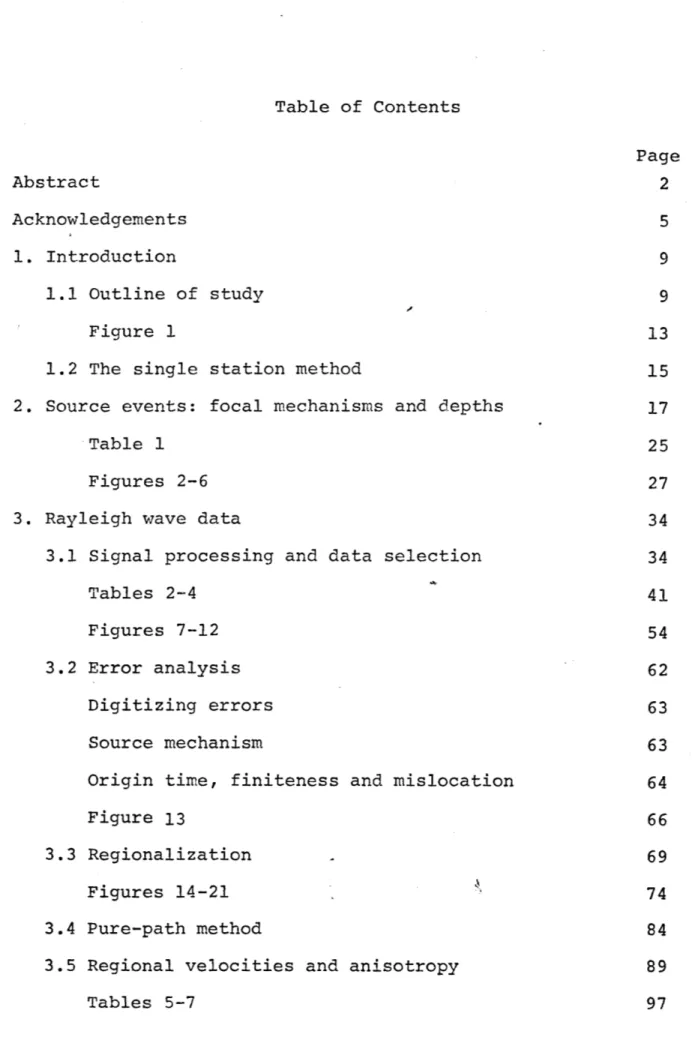
Table of Contents Page Abstract 2 Acknowledgements 5 1. Introduction 9 1.1 Outline of study 9 Figure 1 ₁₃

1.2 The single station method 15

2. Source events: focal mechanisms and depths 17

Table 1 25

Figures 2-6 27

3. Rayleigh wave data 34

3.1 Signal processing and data selection 34

Tables 2-4 41

Figures 7-12 54

3.2 Error analysis 62

Digitizing errors 63

Source mechanism 63

Origin time, finiteness and mislocation 64

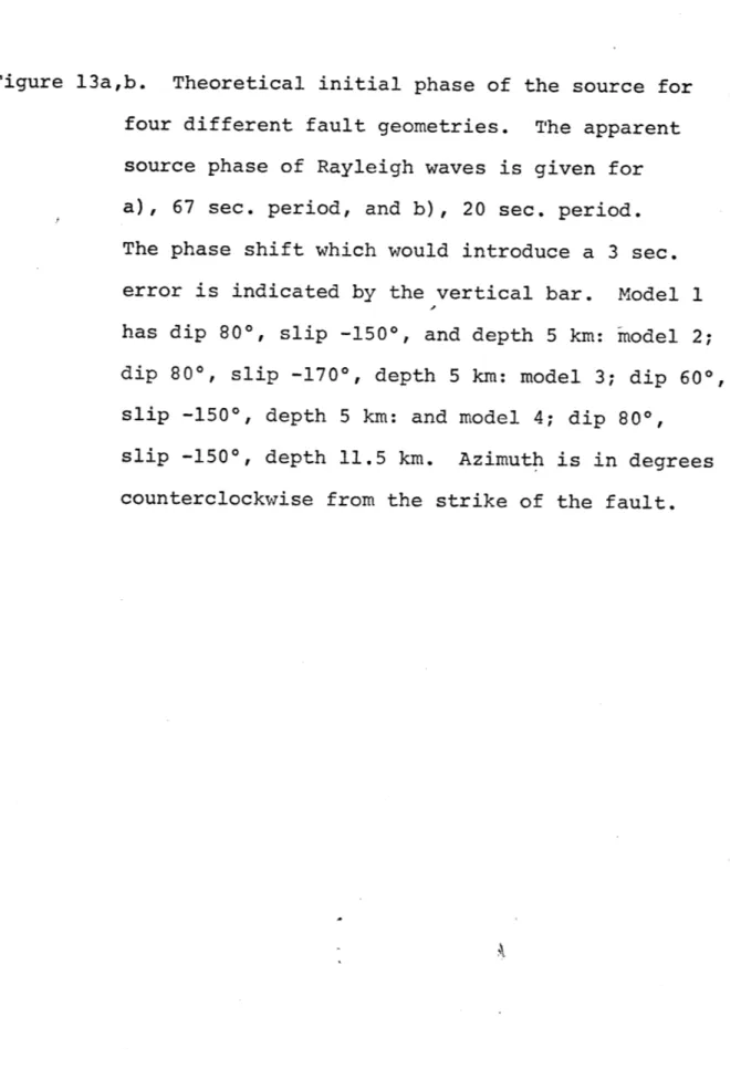
Figure 13 66

3.3 Regionalization 69

Figures 14-21 74

3.4 Pure-path method 84

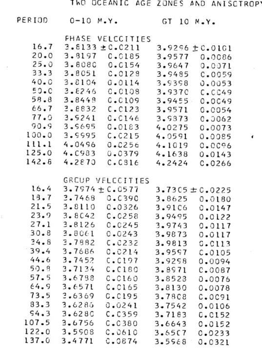
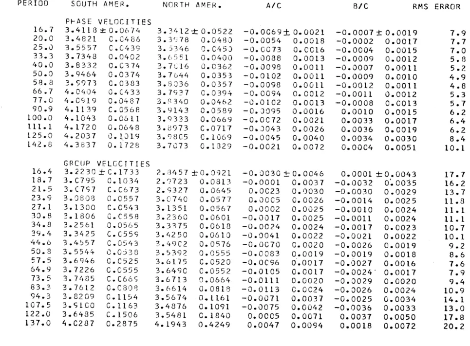
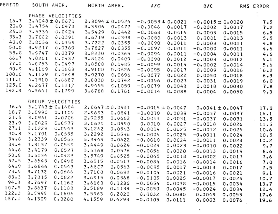
3.5 Regional velocities and anisotropy 89

Page

3.6 Possible systematic errors 102

Mislocation 102

Figure 22 107

Origin time and finiteness 109

Non-horizontally layered media 113

Horizontal refraction 115

4. Love wave data 120

4.1 Method 121

4.2 Higher mode excitation 125

Figures 23-27 130

4.3 Data selection and processing 137

4.4 Error analysis 138

Tables 8-9 140

4.5 Fundamental mode phase velocity 144

4.6 Higher mode velocity 148

Tables 10-11 153

Figures 28-33 156

4.7 Search for contamination of the fundamental mode 164

Figure 34 168

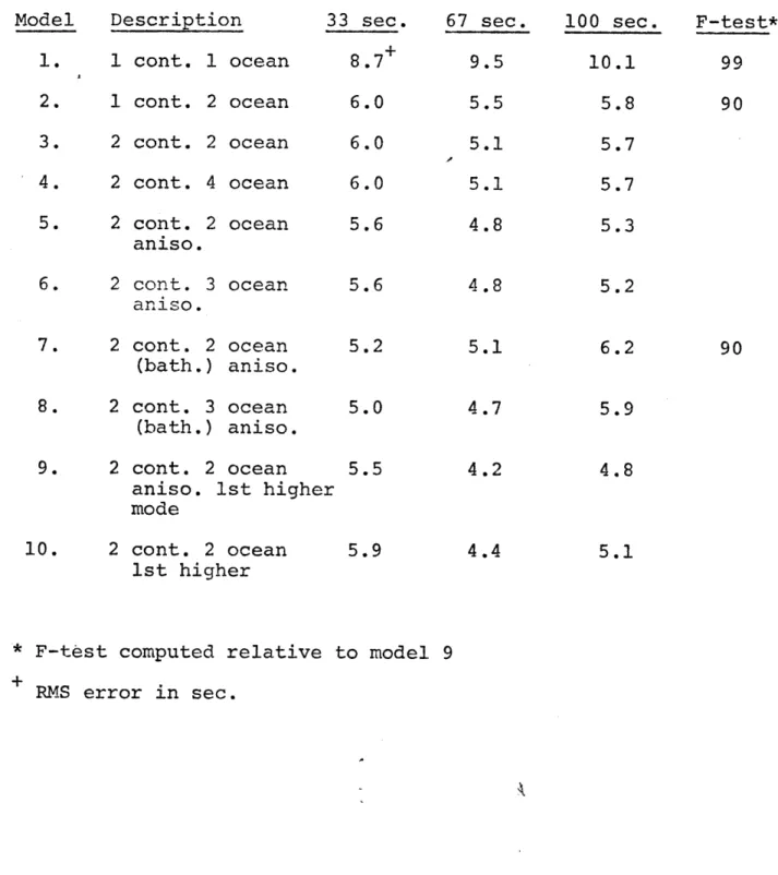
5. Models of the upper mantle 170

5.1 Inversion technique 171

5.2 The starting model 175

Crust 175

Page

Table 12 178

5.3 The evolving structure of the mantle 180

Table 13 190 Figures 35-39 191 5.4 Anisotropy 200 Figures 40-43 211 6. Summary 216 References 220 Appendix 1 234 Figure Al 238 Appendix 2 239 Figures 240 Appendix 3 252 Figure A2 254 Figure A3 255

9.

1. Introduction

1.1 Outline of Study

Hot mantle material rises under mid-ocean ridges to form the new oceanic lithosphere. As the lithospheric plates

spread away from the ridges, the mantle cools, causing a

number of temperature-dependent changes in physical properties of the lithosphere and asthenosphere. Geophysical studies of these changing properties have contributed much to the

understanding of the thermal regime of the mid-ocean ridges and their role in the convective overturn of the mantle. However, most of the observations to date measure only the near-surface effects of the elevated mantle temperatures, such as high heat flow (Lee and Uyeda, 1965; Sclater and Francheteau, 1970) or unusually low P and S velocities

n n

(Talwani, et al., 1965; Keen and Tramontini, 1970; Hart and Press, 1972). Other techniques measure a total effect averaged over a vertical section of the upper mantle.

Gravity anomalies (Talwani et al., 1965), the elevation of the ridges (Sclater et al., 1971), and the attenuation or delay of seismic body waves (Molnar and Oliver, 1969; Solomon, 1973; Long and Mitchell, 1970), all measure in different ways the total changes in density or elastic

properties summed over the upper 100 to 200 km of the oceanic mantle.

10.

by the average properties of the mantle over a large depth

interval. However, by sampling the dispersion of different modes over a wide frequency range, the distribution of shear velocity with depth can be measured. The advantage of

multiple measurements is illustrated in figure 1 by the varying sensitivity of the phase and group velocities of

surface waves to shear velocity structure of the mantle (to a lesser extent, Rayleigh waves depend on the density and compressional velocity, and Love waves depend somewhat on the density). At 40 sec, the phase and group velocity of Rayleigh waves are most sensitive to the shear velocity at

a depth of about 50 to 60 km. The depth of the peak sensitivity increases with period, roughly in proportion to the increase in wavelength. Thus, measurements at different frequencies give averages over different depth ranges. The group velocity, which is related to the derivative of the phase velocity with respect to frequency, is more sensitive to the structure than the phase velocity. Unless the phase velocity is perfectly known over the entire range of frequencies sampled, an

independent measurement of the group velocity can add important information. Phase velocity measurements are needed because it is possible to have two structures with similar group velocities but different phase velocities. The dispersion of Love waves yields additional information. In particular, the phase velocity

11.

of the first higher Love mode is most sensitive to the structure within the low velocity zone of the mantle and if it can be

measured with sufficient accuracy, it will give unique data on the deeper structure beneath the mid-ocean ridges. The higher mode Rayleigh waves are not considered because they are not sufficiently excited by moderate-sized earthquakes to be a significant contribution to the typical sesimic record. Due to the existence of different modes of propagation and a readily observable range of frequencies, surface waves can be used to directly detect the depth distribution of the thermal anomalies associated with the mid-ocean ridges.

The purpose of this study is to measure the dispersion of Rayleigh and Love waves as a function of the age of the sea-floor, in order to determine the structure of the upper mantle beneath a mid-ocean ridge and the changes that occur

in an oceanic plate as it moves away from the ridge. The most rapid changes are expected within the first few million years

(Forsyth and Press, 1971) after formation of the oceanic crust. This study therefore concentrates on the surface wave dispersion within the east Pacific. Here the separation rates between the Nazca and Pacific plates are the highest in the world (Herron,

1972), allowing the most detailed examination of the early

evolution of the lithosphere. In addition to changes with age of the sea floor, the possibility that surface wave

12.

velocities depend on the direction of propagation is considered. Raitt et al. (1969) and Morris et al. (1969) have shown that the Pacific mantle immediately beneath the Moho is anisotropic. If this anisotropy continues to an appreciable depth, it should affect the surface wave velocities, creating the possibility of mistakenly attributing directional variations to regional changes. There have been several previous, regional, surface-wave studies in the Pacific (Kuo et al., 1962; Santo and

Sato, 1963; Savage and White, 1969; Knopoff et al., 1970; Kausel, 1972; Leeds, 1973; and others): none has considered the possibility of anisotropy or simultaneously measured regional phase and group velocities or measured the phase velocity of the first higher Love mode. The results of these

previous investigations are compared with the results of this study later in the text.

The two-station method of measuring phase velocity (Brune et al., 1960) is inadequate for the purposes of this study. There are very few island stations, so the number of possible

two-station paths within the ocean is very limited. In addition, the technique I employ for measuring the phase velocity of the first higher Love mode is possible only using the single station method, in which the phase velocity is computed for a path

13.

Figure 1. Partial derivatives of surface wave velocities at 40 seconds period with respect to shear wave velocity S(z). Steps in the curves are due to discontinuities in the model of the upper mantle. Curve labelled R is the derivative of the

u

fundamental mode Rayleigh wave group velocity;

Rc, fundamental mode, Rayleigh wave phase velocity;

Lo, fundamental mode, Love wave phase velocity; Ll, first higher mode, Love wave phase velocity.

dV /d9

1.0

2.0

100-E

200-

H-L.

O

300-

15.

1.2 The single station method

The technique for measuring phase velocities using only one station was originally developed by Brune et al. (1960). Early studies using this method (Kuo et al., 1962) were hampered by the necessity of choosing an arbitrary initial phase which was independent of period. Subsequent developments in the theory of the excitation of surface waves (Haskell, 1964; Ben-Menahem and Harkrider, 1964; Saito, 1967) have made it possible to compute the initial phase as a function of frequency for an arbitrarily oriented point source in realistic earth models. Recently, Knopoff and others have extensively employed this method in regional studies of the earth (for review, see

Knopoff, 1972; also Kausel, 1972; Weidner, 1972).

The phase velocity between the earthquake and the station is given by

w

DIST

(I)

O() )+ 0i t,- O() (w)

O

n

obs

where DIST is the distance between source and receiver, w is

the frequency, and t_{1 is the time to the beginning of the record.} For convenience, throughout this paper the observed _phase

_#obs'

the phase delay due to instrument response inst , and the initial phase at the source

#

16.

shift. This ambiguity is removed by placing limits on the acceptable value of c at long periods.

#obs

t

,A

(w) e2

obs

=

(t)

e~

d t

(2)

Because the initial phase depends on-the depth and the orientation of the source, the first requirement for -a study based on the

single station method is a set of reliable focal mechanism solutions. The determination of the source geometries and the steps used in signal processing are described in the following sections.

17.

2. Source events: Focal mechanisms and depths

Seventeen earthquakes were used as sources for the single-station study of phase and group velocities. The focal

mechanisms of fourteen of these events were based on both P-wave first motions and the azimuthal variation in surface wave amplitudes. The source parameters for the three events determined from body wave observations alone (events 13, 14 and 16 in Table 1) were given by Anderson and Sclater (1972).

A list of the earthquakes and source characteristics are given

in Table 1. As shown in figure 2, two of the events are intra-plate earthquakes characterized by thrust-faulting, one event associated with the Galapagos Rift Zone is

characterized by normal faulting, the rest, which show

predominantly strike slip motion, are associated with transform faults of the active ridge system of the East Pacific. The remote location and small size of these earthquakes make it difficult to obtain sufficient observations to allow a

satis-factory determination of the focal mechanism from body waves alone. _{However, by combining the first motion observations} of P-waves with the fitting of theoretical radiation patterns to the observed distribution of Rayleigh wave amplitudes, it is possible to accurately describe the geometry of the source. The steps involved in the focal mechanism determination for events 1-12 and 15 are described in the following paragraphs.

18.

(1) Measurement of observed Rayleigh wave radiation patterns.

The long period vertical component of seismograph records of WWSSN stations are digitized at regular time intervals

of 1.0 to 2.0 sec. Records from 20 to 25 stations were Fourier-analyzed for each event, except for the March 7, 1963 earthquake for which only 13 records were available. Using the amplitude equalization method (Aki, 1966), the amplitude spectral densities observed at each station are corrected for geometrical spreading on the spherical earth and for attenuation. Hagiwara's formula

(Hagiwara, 1958) is employed to correct for instrument response. These corrected amplitudes, plotted as a function of azimuth from the source to the station, form a radiation pattern which is dependent on the strike and dip of the fault plane, the direction of the slip on the fault, the source depth, and

the medium in which the earthquake occurs. For Rayleigh waves at long periods, a shallow, strike-slip source yields a four

lobed pattern, with the nodes in the direction of the strikes of the fault and auxiliary planes. A dip-slip event gives a two-lobed radiation pattern. Because long period data is less sensitive to the focal depth and effects of the finiteness of the source, the focal mechanism solutions are primarily

based on the 67 second period radiation patterns. In addition, the lateral heterogeneities of the earth affect the long period data to a lesser degree than at very short periods. At periods

19.

much greater than 67 sec., long period noise reduces the relia-bility of the observed amplitudes. For events 3 and 9, the

50 sec. period data gave slightly better results, but for

all other events, the scatter in the 67 sec. period amplitudes was less than or equal to the scatter in the shorter period data. In correcting for the attenuation, I assume a Q value

of 125 (Ben-Menahem, 1965) and a group velocity of 4.0 km/sec

for 50 and 67 sec. periods. The solutions were found to be insensitive to reasonable variations in Q. The focal depths are based primarily on the 20 sec. period Rayleigh wave ampli-tudes for which Q is assumed to be 500 (Tsai and Aki, 1969). The seismic moments computed from the 67 and 20 sec. data were found to agree within 10% for these assumed Q values,

suggesting that at least the relative values of Q are accurate. (2) Generation of theoretical radiation patterns.

A number of authors have treated the problem of the

excita-tion of surface waves by an earthquake. I use the results of Saito (1967) as discussed by Tsai and Aki (1970). The fault plane geometry and coordinate system used throughout this paper are defined in Appendix 1. Also given are the

equations describing the excitation of Love and Rayleigh waves

by a double couple, point force in a layered medium. These

equations are used in computing the initial phase of the source as well as the theoretical amplitude radiation patterns.

Using'the oceanic earth model by Harkrider and Anderson

20.

of radiation patterns for a wide variety of source geometries.

3. _{km is the approximate depth to the ridge axis, where the source}

events occur. The shape of each pattern depends only on the depth, and the dip and slip angles. The seismic moment is a scalar factor which is adjusted for each trial pattern to best fit the observed amplitudes. A change in strike corresponds to a rotation of the pattern, so it is not necessary to generate a new pattern for each trial value of the strike of fault plane. The least squares fit of each theoretical pattern to the observed data is computed, then a statistical test is used to define the

family of acceptable models. Most of the earthquakes used as sources occur near the ridge axis. In a later section, I show that the Harkrider-Anderson average ocean model is not a good description of the mantle in the source region. However, neither the shape of the Rayleigh wave amplitude patterns nor the initial phase is very sensitive to the details of the structure (Tsai

and Aki, 1970, Mendiguren, 1971; Weidner, 1972) and no significant error is introduced by using the standard ocean model.

(3) Defining the family of acceptable source geometries.

It is possible using the Rayleigh wave amplitudes to accurately define the source mechanism even for some small events for which there are very few reliable observations of first motion polarities.

For example, the smallest event studied, Sept. 9, 1969, can be shown to be predominantly strike-slip with an uncertainty

21.

in the strike of only ± 9 degrees, despite the fact that there

are only 6 reliable first motion observations (figure 3). The process of defining the limits on the fault parameters

is illustrated in figure 4. The least squares fit of three radiation patterns is plotted versus assumed strike of the fault plane. After the best model is found, anF-test is per-formed comparing the fit of all othei models with the best

model. With 26 data, in this case, and the one scalar variable, the seismic moment, a ratio of 1.95 between the sum of the

squares of the errors for a trial model and the best fitting model means there is only a 5% chance that the difference in fit is due to random fluctuations in the data. In other words, the best pattern is a significantly better model of

the source at the 95% confidence level. In figure 4, the best model has dip, 80*, slip, -165* and strike, 100*, but a pure strike-slip source cannot be rejected. A dip of 60* and slip of -150* is unacceptable. In this way, a range of possible models is defined, with limits set at the boundaries

of the 95% confidence region in the three-dimensional space of the fault parameters, strike, slip, and dip. As in this example, the strike of a predominantly strike-slip source

is usually well-determined, while the dip and slip are somewhat more uncertain. The data used for each of the earthquakes

is given in Appendix 2. For purposes of determining the region of acceptable models, a depth of 5 km below sea bottom (base

22.

of the crust) was assigned to each event, following the results of Weidner and Aki (1973) and Tsai (1969). Although variation of a few kilometers in depth affects the quality of the fit, the best fitting source mechanism to the long period data is usually not significantly altered. Further tests (paragraph 5)

justify the assigned depth.

(4) Compatibility with first m6tion observations. The fitting of radiation patterns within the three

dimensional space of fault parameters is a non-linear problem leading to regions of local minima in the error. Some first motion observations or other independent information are required in choosing the correct local minima. For example, a pure thrust event will yield the same two-lobed pattern

characteristic of pure normal faulting. Generally it requires only a few P-wave observations to resolve this ambiguity. The last step, then, is to choose a model consistent with the

first motions which is as close as possible to the center of the region of possible models. In every case, a solution was found which was consistent with the body wave data and within the range of possible models defined by the Rayleigh wave amplitudes. A further check on the solutions is provided

by the observations of Love and Rayleigh phase velocities.

If, due to an error in the source mechanism, the azimuth from the epicenter to the station is assigned to the wrong quadrant, an error of 7r _{will result in the initial phase. Such an error}

23.

is easily detected at long periods, yet no such mistake was found.

(5) Determination of focal depth.

The shape of the radiation pattern from pure strike-slip motion on a vertical fault is independent of depth; the

shape from pure dip-slip motion on a fault dipping at 45* varies only slowly with depth. In these two cases, measuring depth with surface waves is possible only by observing the

changes in amplitude with period, requiring a precise knowledge of the effects of attenuation and the transfer function for the continent to ocean transition (or by measuring the 7 phase shift that occurs when the hypocenter is deeper than the change from retrograde to prograde particle motion). For shallow

events, amplitudes for periods of 10-20 sec. are required, yet for oceanic paths, there is a great deal of scatter in the amplitudes for periods less than 20 seconds (personal

observations and Weidner, 1972). For these reasons, I believe the most precise depth determinations can be made only for

earthquakes with components of both dip and strike-slip motion. The radiation pattern at periods of 20 sec. or less for this type of event varies rapidly with depth and the gross changes in shape can easily be detected despite scatter in the data and uncertainty in the attenuation correction (Mendiguren,

1971).

24.

dip and strike-slip motion is event 4, Nov. 6, 1965. Using only the 20 sec. period data, the depth of the earthquake is restricted to less than 11 km. This limit is established at the 95% confidence level. As shown in figure 5, the best fitting model is the 5 km source depth, which is consistent with the results of Weidner and Aki (1973) for the mid-Atlantic ridge and those of Thatcher and Brune (1970) in the Gulf of California. The seismic moment for the best fitting model,

9.2 x 1024 dyne-cm, is very close to the seismic moment

estimated from the 67 sec. data (Table 1), indicating that the choice of Q is approximately correct. For purposes of computing initial phase, all events were assigned a focal depth of 5 km, except event 17, which was shown by Mendiguren to be 9 km beneath the ocean bottom. The initial phase of a pure strike-slip event is independent of depth, so that no error is introduced by

misassignment of the focal depth for such an event. The initial phase, like the amplitude radiation pattern, is most sensitive to depth if the earthquake is characterized by components of both dip and strike-slip motion. However, as discussed above, the sensitivity of the radiation pattern for these events provides good control on the source depth. The effect of the uncertainties in focal depth and mechanism on the initial phase are discussed later in the section on error analysis.

25.

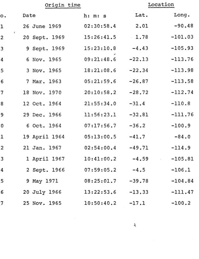
Table 1. Earthquake source characteristics

Origin time No. 1 2 3 4 5 6 7 8 9 10 11 12 13 14 15 16 17 Date 26 June 1969 20 Sept. 1969 9 Sept. 1969 6 Nov. 1965 3 Nov. 1965 7 Mar. 1963 18 Nov. 1970 12 Oct. 1964 29 Dec. 1966 6 Oct. 1964 19 April 1964 21 Jan. 1967 1 April 1967 2 Sept. 1966 9 May 1971 20 July 1966 25 Nov. 1965 h: m: s 02: 30: 58 .4 15:26:41.5 15:23:10.8 09:21:48.6 18:21:08.6 05:21:59.6 20:10: 58.2 21: 55:34 .0 11:56:23.1 07:17:56.7 05:13:00.5 02:54:00.4 10:41: 00.2 07:59:05.2 08: 25: 01.7 13:22:53.6 10:50:40.2 Location Lat. Long. 2.01 -90.48 1.78 -101.03 -4.43 -105.93 -22.13 -113.76 -22.34 -113.98 -26.87 -113.58 -28.72 -112.74 -31.4 -110.8 -32.81 -111.76 -36.2 -100.9 -41.7 -84.0 -49.71 -114.9 -4.59 -105.81 -4.5 -106.1 -39.78 -104.84 -13.33 -111.47 -17.1 -100.2

26.

Table 1. Earthquake source characteristics (cont.)

Fault parameters No. strike dip slip

1 175 80 -160 2 204 60 -75 3 100 80 -165 4 52 60 166 5 65 85 165 6 110 82 -8 7 119 80 -6 8 249 87 167 9 50 60 -160 10 268 58 -12 11 271 62 -11 12 108 90 172 13 103 90 180 14 104 90 180 15 196 60 90 16 103 90 180 17 202 46 68 Magnitude Mb 5.0 5.5 5.2 6.2 5.8 5.6 6.0 5.4 5.5 5.5 5.4 5.0 5.1 6.2 4.8 5.7 Seismic moment 1025 dyne-cm. 0.60 2.73 0.48 0.96 1.94 7.64 1.37 2.40 2.16 2.93 0.94 3.96 8.96

27.

Figure 2. Focal mechanisms of earthquakes in the east Pacific used as sources for Love or Rayleigh waves. In the projections of the lower focal hemisphere, shaded quadrants represent

compressional first motions. Double lines are spreading centers, single lines are transform faults.

Figure 3. Focal mechanism of the Sept. 9, 1969 earthquake. In the left hand figure, dots indicate observed amplitudeos of 50-sec. Rayleigh waves as function of azimuth. The amplitude is proportional to the distance from the center of the figure. Smooth, continuous line is the theoretical radiation pattern. Figure on the right is a Schmidt net projection of the lower focal hemisphere showing the distribution of P-wave

polarities. Solid circles represent compressional arrivals, open circles are dilatational. Smaller symbols indicate less reliable observations.

Figure 4. Sum of the squares of the residuals in amplitude for three trial values of dip and slip. A dip of 80*, slip of -165*, and strike of 100* gives the best fit to the observed amplitudes of the Sept. 9, 1969 event. Scale for sum of squares

Figure 5.

Figure 6.

is arbitrary. Dotted line gives 95% confidence limit discussed in text.

Sum of squares of residuals in amplitude given as a function of model source depth. Best fit to observed 20 sec. period amplitudes is at about

5 km. with strike, dip and slip held at 520,

600, and 1664, ctively. The 95%

confidence limit on the depth of the Nov. 6,

1965 event is 10.5 km. Vertical scale is arbitrary.

Vertical component of Rayleigh wave observed at Tucson from March 7, 1963 event. Motion toward top of figure is upward. Horizontal scale gives group arrival time in km/sec. Time between tick marks is 1 minute. Note apparent long period undulation superimposed on shorter period oscillations between 3.8 and 3.6 km/sec.

uN

0

0)

Ii..

0

N

aw

CL

w

CL

z

i-rn

Si

0~

9, 1969

Q

= 125

DEPTH

=5

DIP= 80

SLIP= -165

60 -150

\

90 -180

80 -165

9-9-69

50 sec

Q= 125

70

₉₀

₁₁₀

₁₃₀

STRIKE

_DEG

3.0

U)

w

0

Uo

2.0

1.0

0.01

2.0

1-0.95

w

0:.

U)

0

11-6-65

20 sec

Q 500

=

52

=

60

X=166

0.0

I

0

5

10

15

DEPTH

_km

TUC

3/7/63

---- .--- ""

em

I

I

I

3 *2

34.

3. Rayleigh wave data

3.1 Signal processing and data selection

The digitized records used in the focal mechanism study form the primary data base for the measurement of the phase and group velocities. The length of the digitized record depends on the dispersive character and length of each path, but most often is 8 to 10 minutes long. I started one to two minutes before the onset of the Rayleigh wave, which is usually very clear, and continued past the arrival time of

15 sec. period waves. For example, for the record shown in

figure 6, I digitized from the left to the right hand

side of the figure, for a total record length of about 8 minutes. Many of the stations are not considered in this portion of

the study, because only relatively simple paths with a high percentage of ocean were desired. Stations that met this

requirement for some or all of the sources were ALQ, TUC,

BKS, and GSC in North America, BHP and LPS in Central America, GIE in the Galapagos Islands, and BOG, QUI, NNA, ARE, LPB,

ANT, and PEL on the west coast of South America (figure 12).

The diagram in figure 7 outlines the steps employed in selecting and processing the data after the digitized signal is obtained. Only the first 3 boxes apply to the treatment of Love wave

data, which will be discussed later. The steps are best illus-trated by following an example, such as the path from event

8 on Oct. 12, 1964 to the station at Alburquerque (ALQ).

35.

a study of the ocean floor, so any path which is not predominantly oceanic is of little value. The paths accepted in this study

are on the average 89.5% oceanic. 82.5% of path 8-ALQ is

within the ocean (table 2) which is acceptable. The next test allows for uncertainty in the focal mechanism of the

source. The initial phase of the surface wave changes rapidly with azimuth in the vicinity of a node in the amplitudes.

A small error in the assignment of the strike of the fault

plane can then lead to a large error in the assumed initial phase. To eliminate this possibility, we reject all paths within 100 in azimuth of a node. For a strike-slip event, this eliminates nearly 25% of the possible data. 8-ALQ is

approximately 25* clockwise from the nearest node, passing the test. Following the screening of the paths, the records are Fourier-analyzed (this step is already complete for events 1-12 and 15).

Moving window analysis (Landisman, et al., 1969) is performed on each record. This yields contours of energy levels on

a velocity (travel time) versus log period plot. When corrected for instrument delay, the time of arrival of the peak energy level of a wave packet for a given frequency gives the group velocity at that frequency. All records in this study were analyzed with a cosine-squared window shape and a window length of 4.0 times the period of analysis. I find that normalizing the energy contours relative to the peak amplitude separately

36.

for each period produces a more easily interpretable plot. The results are shown in figure 8 for 8-ALQ. The broken line represents the arrarent group velocity, not corrected for instrument response.

Normally, record 8-ALQ would be rejected at this point on the basis of the holes in the amplitude spectrum and the oscillations in the observed phase (thin lines in figures

9 and 10). These phenomena are characteristics of records showing beating or the interference of two simultaneously arriving signals. However, in this case the moving window analysis shows there are two clearly separated arrivals of energy in the period range 20 to 50 sec. When interference is caused by a distinctly separate signal, the interference can often be removed by time-variable filtering. A frequency-domain time-variable filter (Landisman et al.) based on the moving window analysis is used to extract the desired signal.

With this filter, energy of a particular frequency is allowed to pass only within a specified time window. In the example shown in figure 8, the 40 sec. period signal arriving with an apparent group velocity of 3.4 km/sec would not be passed, but the signal arriving with a group velocity of

3.7 km/sec would be accepted. The window is centered at the

group velocity of the desired signal. The filtering is

37.

a series of sine and cosine coefficients using the fast

Fourier transform algorithm. The filtered seismogram is then constructed from the linear superposition of these harmonic signals (from the Fourier analysis) of period T after they are windowed by the operator.

0

t

< ta #

c

{r

t

DI

ST

/

U(T)

tb-

_ta

t

_>

_tb

ta<

_t

_{< tb}

(3)

= DIST/U(T)

Tta

+d

U(t)

d T

=

DIST /U(T)

+ T

f

a +

d

U(t)

ie d T

'

38.

where T is the period and U(T) is the velocity of the desired signal determined from the moving window analysis. In this study, a = 3.5 and 6 = (DIST x sec 2)/(100 km2) were found to give satisfactory results.

The unfiltered and filtered seismograms for 8-ALQ are shown in figure 11. Periods shorter than about 20 sec. have been eliminated due to the complexity of the energy versus velocity plot at these high frequencies. The relatively high amplitude, long period component is readily apparent

in both the filtered and unfiltered seismograms, and it is also clearly seen in the seismogram for the similar path

6-TUC, shown in figure 6. The minimum in the amplitude

spectrum at about 40 sec. (figure 9) is typical of all paths traveling along a substantial portion of the ridge axis,

but is not found for paths outside this zone. The apparently high amplitude of the long-period signal is actually primarily due to the greater attenuation of the shorter periods, although in this particular case, focusing or defocusing of the signal may also be important (see later discussion of horizontal refraction). The details of the character of the observed amplitude spectra will be the subject of a subsequent study. The phase spectrum of the filtered seismogram shows no

unusual phase shifts (solid line, figure 10) and is therefore passed for further study. The group velocity diagram of 8-ALQ

39.

which I attribute to long period noise, so the final, selected range of acceptable data for 8-ALQ is 20-167 sec. With my

initial selection of the portion of the record to be digitized, time-variable filtering was found to be necessary or useful only when a clearly separable, interfering signal or noise was observed. Thus, the phase and group velocities were

normally derived from unfiltered seismograms. If the

interfering signal was not sufficiently separated in time, the record or portions of it were rejected.

The phase velocity is computed according to (1), the

instrumental phase correction is computed by Hagiwara's (1958) formula as corrected by Brune (1962), and the initial phase for each path follows from the source mechanism and the relations given in Appendix 1. Rayleigh wave phase and group velocities were measured for the 78 paths in the East Pacific area shown in figure 12. The path identification, path length corrected for the ellipticity of the earth, and other descriptive characteristics of the paths are given in Table 2. Group and phase velocities for each path are given

in Tables 3 and 4 respectively. Two of the paths, GI-PEL and GI-ANT are two-station paths. These are processed in the same way as the single station data, except the original, digitized signal is the windowed cross-correlogram of the Rayleigh waves observed at each station. The errors which

40.

may produce scatter in the individual observations of velocity are discussed in the following section.

41.

PATHID TOTAL LENGTH 1-BHP 1-PEL 2-BOG 2-ARE 2- P EL 3-TUC 3-BOG 3-QUI 3-ARE 3-PEL 3-BHP 4-TUC 4-ALO 4-BKS 4-GSC 4-QU I 4-ARE 4-LPB 4-ANT 4-PEL 5-TUC 5-ALQ 5-GSC 5-GIE 5-ARE 5-BHP 6-TUC 6-ALQ 7-TUC 7-ALQ 7-BKS 7-BHP 7-NNA 7-ARE 7-LPB 7-ANT 8-BKS 8-TUC 8-ALQ 1433.7 4412.5 3013.3 3822.8 5C10. 1 4098.7 3682. 3C86.6 3990.0 4844.8 3280.7 6032.8 6363.4 6701.1 6364.4 4527.4 4472.9 4821.0 4433.0 4389.6 6057.3 6389.3 6386.5 3506.3 4495.8 5107.9 6556.2 6882.4 6755.7 7075.3 7436.4 5483.8 4156.1 4427.6 4752.9 4244.2 7760.1 7051.6 7357.8

AGE ZCNES M.Y.

0-5 5-1C 10-20 36.3 336.5 1525.9 278.2 333.1 500.C 1495.1 725.0 309.6 332.1 1396.0 1458.7 2071.3 1067.2 1161.5 633.8 521.1 52C.4 516.1 566.8 1464.6 2079.7 1165.5 764.7 535.5 127C.3 1925.5 2563.0 2296.3 2702.6 1784.7 1421.5 442.9 416.6 413.9 405.3 2141.8 2513.9 4105.7 326.6 165.7 564.4 340.1 407.2 2000.2 671.7 669.3 309.7 332.1 598.3 894. 1 887.7 574.6 429.6 4'9 8.C 409.4 4C8.9 405.5 482.9 897.7 891.3 431.1 651.5 420.7 1172.6 992.0 1098.4 1182.9 1103.9 594.9 834.8 443.0 416.6 414.0 405.4 535.4 1540.8 3C9.0 660.3 0.0 0.0 755.0 687.0 778.8 543.2 864.0 887.3 1630.7 859.0 2654.4 2163.6 1641.8 3118.6 1442.5 1501.5 1510.2 1456.5 1484.4 2665.2 2172.4 3129.4 2090. 1 1495.1 2163.4 2539.7 1961.5 2229.4 1981.1 1636.0 2179.3 1569.7 1410.4 1417.5 1347.2 1668.4 1939.2 1655.5

BATHYMETRIC ZONES KM. AZIMUTHA

GT 20 LT 3.5 3.5-4.0 GT 4.0 CS 77.3 3701.0 506.2 1646.8 3393.4 c.0 489.5 518.4 2001.0 2366.1 9C. 7 0.0 C. c 3C49. 0 954.7 1553. C 1839.9 1885 .1 200 1. 9 1696.5 c. 0 C.0 95E.0 C. 0 1817.3 183.8 0.0 0.0 C.0 C .0 3048.9 781.7 1563.8 20C5.4 2042.9 2C20.7 3026.4 C.0 0.0 1100.5 765.0 2596.5 724.8 467.6 721.4 2633.2 2032.5 315.7 ?28.4 2723.2 1972.8 2049.0 981.6 1076.2 648.0 239.2 246.5 258.4 389.2 1970.8 1995.6 1080.0 743.3 264.7 2026.2 2621.4 2631.5 2968.5 2951.7 1752.0 1966.9 824.0 1126.0 1179.3 819.0 2145.3 2409.5 2124.6 0.0 1160.1 0.0 942.3 1711.3 2295.3 566.3 744.2 957.6 2134.7 220.8 2258.2 2602.3 1868.1 2532.0 1679.8 320.4 324.3 2C41.1 2953.0 2161.8 2659.1 2495.3 1542.8 354.3 1590.3 2158.8 2620.3 2163.6 2529.2 1886.2 1513.0 884.3 743.6 857.7 3359.6 1909.3 3200.7 3605.7 0.0 2278.1 0.0 1353.0 2641.8 262.3 0.0 0.C 2234.3 2297.8 0.0 776.1 471.3 3482.9 2056.2 1799.5 3712.2 3753.8 2C80.5 888.4 894.9 488.6 2108.8 1220.2 3649.7 1173.6 726.9 371.1 576.6 306.7 3426..3 1737.4 2311.1 2379.4 2251.4 0.0 3317.4 383.6 339.9 0.428 0.508 0.858 -0.329 0.237 0.765 0.047 -0.273 -0.681 -0.120 0.228 0.809 0.780 0.574 0.772 -0.277 -0.90C -0.859 -0.987 -0.838 0.609 0.780 0.774 0.144 -0.893 0.112 0.815 0.799 0.812 0.800 0.592 0.192 -0.518 -0.760 -0.752 -0.945 0.588 0.814 0.797 L CONTINENTAL SN S.A. N.A. -0.637 -0.523 -0.079 -0.713 -0.929 -0.184 0.083 0.159 -0.548 -0.952 -0.036 -0. 137 -0.034 -0.674 -0.429 0.865 0.314 0.255 -0.036 -0.474 -0.135 -0.036 -0.426 0.907 0.317 0.388 -0.157 0.012 -0.171 0.022 -0.671 0.453 0.815 0.586 0.498 0.278 -0.676 -0.204 -0.039 333.1 209.3 416.9 802.6 189.5 0.0 483.5 309.9 482.4 183.8 336.7 0.0 0.0 0.0 0.0 400.1 200.9 496.4 53.0 159.0 0.0 0.0 0.0 0.0 227.2 317.8 0.0 0.0 0.0 0.0 0.0 266.5 136.8 178.5 464.6 65.6 0.0 0.0 0.0 0.0 0.0 0.0 0.0 0.0 819.7 0.0 0.0 0.0 0.0 0.0 1025.6 1240.9 368.6 700.1 0.0 0.0 0.0 0.0 0.0 1029.7 1245.9 702.5 0.0 0.0 0.0 1049.0 1259.5 1047.1 1287.7 371.8 0.0 0.0 0.0 0.0 0.0 388.0 1057.7 1287.6

PATHID TOTAL LENGTH 8-GIE 8-BHP 8-QUI 8-ANT 8-PEL 9-BK S 9-GSC 9-TUC 9-ALQ 9-NNA 9-ARE 9-LPB 9-PEL 10-GIE 1O-QUI 10-BOG 10-NNA 10-ARE 10-LPR IC-ANT i-QUI 11-NNA I1-ARE 11-ANT 11-PEL 12-TUC 12-GSC 13-TUC 15-ARE 15-LPB 15-GIE 16-ALQ 16-TUC 16-GSC 17-ANT 17-LPB 17-ARE GI-PEL GI-ANT 4025.2 5573.2 4851.2 4059.3 3765.1 7900.6 7558.2 7208.7 7520.3 42.39.0 4426.4 4732.1 3814.7 4077.1 4610.3 5314.9 3609.5 3637.0 3903.3 3235.6 4625.8 3362.0 3040.0 2357.8 1508.4 9094.0 9418.6 4117.6 4131.6 4384.7 4569.1 5368.6 5C51 .0 5411.7 3187.2 3418.5 3058.8 4132.8 3326.8

AGE ZONES M.Y. 0-5 5-IC 10-20 404.3 1156.7 348.7 372.0 393.2 2218.5 2620.8 2876.3 3943.7 405.0 413.5 423.1 547.1 113.1 106.4 10S.3 130.6 157.5 154.7 214.1 1C6 .2 112.1 124.2 142.2 233.4 4161.9 2196.4 502.3 165.2 153.4 143.3 996.7 500.0 71S.7 0.0 c.C 0.0 C.0 C.0 750.9 765.1 481.6 372.0 393.2 625.7 137.9 1232.7 342.9 373.8 413.5 423.2 547.1 229.6 106.4 109.4 130.6 157.5 154.7 214.1 0.0 0.0 C.0 0.0 0.0 976.2 1947.8 20C.4 165.3 153.4 290.8 1123.9 1166.8 308.5 0.0 0.0 0.0 132.2 186.3' 2870.0 1972.9 1868.1 1238.0 1780.7 1619.6 3174.4 2054.5 1917.7 1551.7 1392.2 1251.6 1530.7 3060.8 1566.3 1472.1 1110.2 891.4 833.0 713.7 595.9 507.2 366.7 290.3 173.6 2910.1 3089.3 782.3 1322.1 1315.4 3655.3 1959.5 2323.5 3598.8 1070.9 977.7 978.8 132.2 0.0 BATHYMFTRIC ZONES KM. GT 20 LT 3.5 3.5-4.0 GT 4.0 c.0 1337.6 1631.0 2017.7 1C45.0 3065.4 907.0 C.0 0.0 1765.7 2028.8 2169.3 1C28. 3 673.6 2CS8.3 2063.3 2083.8 2252.3 2296.8 2016.3 2802.6 2548.1 2348.1 1765.4 814.1 C.0 1507.0 0.0 2313.7 2302.0 475.8 c.0 C.0 C.0 2062.1 188C .2 182C.0 3595.7 306C.7 998.2 2251.3 822.6 540.0 795.5 2243.7 2318.8 3402.3 2736.1 737.3 6'66.9 682.8 1015.6 448.5 135.7 142.7 145.1 179.9 223.5 284.2 59.6 57.0 51.1 46.2 61.1 4080.4 2569.7 774.1 245.9 306.1 685.4 1228.1 1276.9 485.8 0.0 0.0 0.0 347.8 487.0 1618.1 1534.2 1450.3 3459.7 2386.6 1739.2 2626.6 2225.0 3133.2 1146.9 1669.5 2261.6 2181.0 1961.1 1298.9 1321.4 1478.8 2040.6 2283.6 2874.0 1184.6 1111.8 871.6 764.9 0.0 3179.0 3889.5 2256.4 2609.8 2833.3 2627.3 2529.7 2202.6 3035.3 282.0 120.0 148.3 1255.8 357.2 1408.8 1486.8 2056.5 0.0 433.9 3546.2 1894.7 536.2 335.0 2211.9 1911.6 1322.8 456.6 1667.5 2442.8 2290.0 1831.2 1238.2 932.0 0.0 2260.5 1998.6 1916.3 1386.9 1160.0 788.7 2281.3 263.5 1110.5 784.8 1256.5 322.3 510.8 1105.9 2851.0 2737.8 2650.4 2260.4 2402.8 AZIMUTHAL CS S 0.548 0. 0.288 0. 0.090 0. -0.897 0. -0.955 -0. 0.603 -0. 0.778 -0. 0.822 -0. 0.803 -0. -0.331 0. -0.622 0. -0.642 0. -0.958 -0. 0.850 -0. 0.417 0. 0.303 0. 0.079 0. -0.326 0. -0.410 0. -0.676 0. 0.701 0. 0.787 0. 0.489 0. 0.208 0. -0.338 0. 0.848 -0. 0.819 -0. 0.765 -0. -0.246 0. -0.335 0. 0.843 0. 0.738 0. 0.768 -0. 0.722 -0. -0.842 -0. -0.833 -0. -0.913 -0. 0.598 -0. 0.322 -0. CONTINENTAL N S.A. N.A. 761 671 887 406 093 669 452 194 030 907 731 633 002 406 730 638 953 893 780 704 288 518 796 909 736 201 432 185 928 830 490 054 132 433 505 044 020 719 919 0.0 301.0 521.9 59.5 148.9 0.0 0.0 0.0 0.0 142.7 178.5 464.9 161.4 0.0 732.9 1560.8 154.4 178.3 464.1 77.3 1121.0 194.6 201.1 160.0 287.3 0.0 0.0 0.0 165.3 460..4 0.0 0.0 0.C 0.0 54.2 560.6 260.0 268.6 79.8 0.0 0.0 0.0 0.0 0.0 371.3 718.0 1045.3 1316.1 0.0 0.0 0.0 0.0 0.0 0.0 0.0 0.0 0.0 0.0 0.0 0.0 0.0 0.0 0.0 0.0 1045.8 678.1 823.5 0.0 0.0 0.0 1288.5 1060.7 784.7 0.0 0.0 0.0 0.0 0.0

44.

PERIOD 1-BHP -PEL 2-80G 2-ARE 2-PEL 3-TUC 3-BOG 3-UI _{3-ARE 3-PEL 3-BHP} 16.4 18.7 21.5 23.9 27. 1 30.8 34.8 39.4 44.6 50.8 57.5 64.9 73.5 83.3 94.3 107.5 122.0 137.0 156.2 3.33 3.39 3.43 3.48 3.52 3.57 3.60 3.61 3.58 3.55 3.49 3.47 3.44 0.0 0.0 0.0 0.0 C.0 0.0 3.72 3.75 3.81 3 -907 3.91 3.90 3.90 3.90 3.84 3.75 3. 7C 3.65 0.C 0.C 0.0 cC 0.0 0.0 0.0 0.0 3.62 3.69 3.71 3.73 3.77 3.78 3.75 3.72 3.72 3.74

a.C

4-TUC 4-ALQ 4-BKS 4-GSC 4-QLI 4-ARE 4-LPB _{4-ANT 4-PEL}

5-TUC 5-GSC 3059 3.64 3.69 3. 73 3.76 3.78 3.79 3.78 3.76 3.73 3.71 3.7C 3.68 3.66 3.63 0.0 0.0 0.0 0.0 3.*50 3. 54 3.58 3.64 3.70 3.72 3.72 3.73 3. 71 3.68 3.66 3.64 3.62 3.61 3 . 59 3.56 0.0 0.0 3.68 3.76 3.82 3.87 3.89 3.90 3.89 3. 86 3.85 3.83 3.80 3.78 3.75 3.72 3.69 3.65 3.64 0.0 0.C 0.0 3.75 3.80 3.82 3 84 3.84 3.84 3.82 3.81 3.79 3.75 3.72 3. 7C 3.68 3.66 3.64 3.64 3.60 0.0 0.0 3.82 3.8E4 3.87 3.89 3.91 3.91 3. 87 3.86 3.83 3.80 3 76 3 71 3.70 0.C 0 . 0.C 0.C 0. C 3.72 3.77 3.83 3.87 3.91 3.93 3.94 3.93 3.93 3.90 3.87 3.85 3.82 3.80 3.75 0.0 0.0 0.0 0.0 3.70 3.72 3.74 3.76 3.78 3.81 3.82 3.81 3.83 3.83 3.84 3.83 3.80 3.77 3.71 3.68 3.65 3.66 0.0 3.77 3.81 3.86 3.90 3.93 3.95 3.96 3.95 3.94 3.90 3.87 3.85 3.80 3.71 3.67 3.63 0.0 0.0 3.58 3.81 3.85 3.89 3.91 3.92 3.91 3.90 3.88 3.83 3.80 3.76 3.71 3.64 3.58 0.0 0.0 0.0 0.0 3.60 3.70 3.72 3.74 3.76 3.79 3.81 3.80 3.77 3.74 3.73 3.71 3.69 3.68 3.65 3.63 3.60 3.59 0.0 0.0 3.79 3.81 3.83 3.84 3.85 3.85 3.84 3.82 3.79 3.77 3.73 3.70 3.69 3.66 3.64 3.61 3.58 0.0 3.59 3.64 3.66 3.70 3.72 3.72 3.70 3.71 3.72 3.72 3.73 3.72 3.72 3.73 3.75 3.78 0.0 0.0 0.0 PERIOD 16.4 18.7 21.5 23.9 27.1 30.8 34.8 39.4 44.6 50.8 57.5 64.9 73.5 83.3 94.3 107.5 122.0 137.0

156.2-PERIOD 5-ALO 5-GIF 5-tRE 5-BHP 6-TUC 6-ALQ 7-TUC 7-ALO 7-BKS 7-BHP 7-NNA 16.4 3.51 3.73 0.C 3.69 3.6C 3.55 3.59 3.54 3.70 3.73 3.80 18.7 3.55 3.77 3.79 3.71 3.63 3.58 3.61 3.57 3.75 3.77 3.84 21.5 3.59 3.84 3.84 3.74 3.69 3.61 3.67 3.60 3.83 3.79 3.87 23.9 3.65 3.89 3.87 3.80 3.74 3.66 3.71 3.63 3.85 3.81 3.89 27.1 3.68 3.92 3.90 3.86 3.77 3.69 3.73 3.66 3.86 3.83 3.91 30.8 3.72 3.94 3.93 3.88 3.78 3.71 3.75 3.69 3.87 3.85 3.91 34.8 3.73 3.91 3.94 3.87 3.78 3.73 3.77 3.72 3.88 3.86 3.90 39.4 3.74 3.89 3.94 3.83 3.78 3.73 3.77 3.73 3.87 3.85 3.91 44.6 3.73 3.86 3.93 3.81 3.76 3.72 3.74 3.71 3.84 3.84 3.89 50.8 3.71 3.81 3.88 3.78 3.74 3.70 3.72 3.69 3.79 3.81 3.88 57.5 3.70 C.C 3.83 3.76 3.72 3.68 3.69 3.68 3.74 3.77 3.83 64.9 3.67 0.0 3.80 3.74 3.68 3.68 3.69 3.67 3.73 3.71 3.80 73.5 3.65 0.0 3.78 3.70 3.65 3.66 3.66 3.64 3.72 3.65 3.78 83.3 3.64 0.0 3.79 3.65 3.62 3.64 3.65 3.62 3.72 0.0 3.78 94.3 3.65 0.0 0.0 0.0 3.62 3.62 3.64 3.63 0.0 0.0 3.78 107.5 3.66 0.0 0.0 0.0 3.62 3.59 3.62 3.63 0.0 0.0 3.79 122.0 3.67 0.0 0.0 0.0 3.62 3.57 0.0 3.63 0.0 0.0 0.0 137.0 3.67 0.0 0.0 0.0 3.61 3.56 0.0 3.63 0.0 0.0 0.0 156.2 3.66 0.0 0.0 0.0 3.59 0.0 0.0 0.0 0.0 0.0 0.0

PERIOD 7-ARF 7-LPB 7-ANT 8-BKS 8-TLC 8-ALQ 8-GIE 8-BHP 8-QUI 8-ANT 8-PEL

16.4 3.71 0.0 3.77 3.7C i.64 0.0 3.74 3.79 0.0 3.82 3.77 18.7 3.75 3.72 3.79 3.78 3.68 3.65 3.80 3.82 0.0 3.85 3.84 21.5 3.90 3.76 3.81 3.81 3.72 3.66 3.83 3.85 0.0 3.89 3.88 23.9 3.83 3.77 3.85 3.83 3.74 3.68- 3.86 3.86 0.0 3.91 3.90 27.1 3.87 3.78 3.87 3.85 3.76 3.70 3.87 3.86 0.0 3.93 3.94 30.8 3.9L 3.78 3.9C 3.86 3.78 3.72 3.88 3.85 3.85 3.95 3.95 34.8 3.91 3.79 3.90 3.87 3.77 3.73 3.86 3.83 3.85 3.93 3.94 39.4 3.90 3.80 3.89 3.85 3.75 3.73 3.83 3.80 3.86 3.91 3.94 44.6 3.89 3.81 3.87 3.81 3.73 3.71 3.81 3.76 3.86 3.90 3.92 50.8 3.85 3.80 3.85 3.78 3.71 3.69 3.77 3.75 3.84 3.88 3.88 57.5 3.81 3.81 3.84 3.75 3.69 3.67 3.75 3.73 3.78 3.85 3.83 64.9 3.79 3.79 3.83 3.71 3.68 3.64 3.72 3.71 3.75 3.83 3.80 73.5 3.78 3.76 3.82 3.68 3.68 3.64 3.70 3.67 3.73 3.80 3.79 83.3 3.77 3.75 3.80 3.68 3.66 3.62 3.67 3.65 3.74 3.79 3.77 94.3 0.0 3.76 0.0 3.68 3.65 3.60 3.66 3.62 3.74 0.0 3.77 1C7.5 0.0 0.0 0.0 3.68 3.66 3.59 3.62 3.60 3.71 0.0 0.0 122.0 0.0 0.0 0.0 0.0 3.67 3.59 3.56 0.0 3.68 0.0 0.0 137.0 0.0 0.0 0.0 0.0 3.70 3.59 3.48 0.0 3.66 0.0 0.0 156.2 0.0 0.C 0.0 0.0 C.C 3.61 3.46 0.0 3.62 0.0 0.0