Francis LALOE UMR CNRS 5558 Laboratoire de Biométrie et Biologie Evolutive Université Claude Bernard LYON I - Bât G

(1)

THESE

pr´esent´e devant l’UNIVERSITE CLAUDE BERNARD - LYON I

pour l'obtention du

DIPLOME DE DOCTORAT (arrêté du 25 avril 2002) Soutenue le 14 décembre 2005

par

Clément CALENGE

Des outils statistiques pour l'analyse des semis de points dans l'espace Ecologique

(ANNEXES)

Composition du jury

Directeurs : Mme Anne-Béatrice DUFOUR M. Daniel MAILLARD

Rapporteurs : M. Antoine GUISAN M. Patrick DUNCAN Examinateurs : M. Christian GAUTIER

M. Francis LALOE

UMR CNRS 5558

Laboratoire de Biométrie et Biologie Evolutive Université Claude Bernard LYON I - Bât G. Mendel

43, boulevard du 11 novembre 1918 69622 Villeurbanne

(2)

(3)

'())*+ ,- ./ */

( 0 # #

$ ! " # &

/ 1 2 3 4 2 # 2 #

5 5 6! 7 2 82 $ ! ! 9 #

! 2 '()).+ / .,: *)

. 1 # 2 # ; 2

< 2 7 2 82 " $

2

* 1 # 2 # ; 2

<< 1 2 # = 5 7 2

82 $ ! ! 2

- ! 2 # # # 5 2 > 7 2 82

! ! $ 8 2 1 5

'& + 4 2 8 ; " 0

? 1 # # 2 # 2

$ 7 2 82 22 @

8

, &## # 2 3

% ; " % 5 0 $

0 A & 2 9 #B # 7 '()).+ *) ( ()

: &A ; # 2 C A 2 2 D&40

) 7 2 # 2 .

7 2 # 2 -

( 1 2 # 7 # # # 2

& %

/ # 2 = ; "

CA #

(4)

(5)

; " CA # 2 2

; F G7H 2II # I ;I 2 2

* 5 D D % D CA

#

(6)

(7)

% &'(()* +, -. ).

(8)

(9)

K-select analysis: a new method to analyse habitat selection in radio-tracking studies

Clément Calengeâ^,∗, A.B. Dufourâ, D. Maillard^b

aUMR CNRS 5558, Laboratoire de Biom´etrie et de Biologie Evolutive, Universit´e Claude Bernard Lyon 1, 69622 Villeurbanne Cedex, France

bOfﬁce national de la chasse et de la faune sauvage, 95 rue Pierre Flourens, F34098 Montpellier Cedex 05, France Received 5 August 2004; received in revised form 3 December 2004; accepted 13 December 2004

Abstract

Two kinds of wildlife habitat studies can be distinguished in the literature: hindcasting and forecasting studies. Hindcast- ing studies aim to emphasize among a large set of habitat variables those that are of interest for the focus species, whereas forecasting studies are intended to predict habitat selection according to a small number of habitat variables for a given area.

We provide here a new analytical tool which relies on the concept of ecological niche, the K-select analysis, for hindcasting studies of habitat selection by animals using radio-tracking data. Each habitat variable defines one dimension in the ecological space. For each animal, the difference between the vector of average available habitat conditions and the vector of average used conditions defines the marginality vector. Its size is proportional to the importance of habitat selection, and its direction indicates which variables are selected. By performing a non-centered principal component analysis of the table containing the coordinates of the marginality vectors of each animal (row) on the habitat variables (column), the K-select analysis returns a linear combination of habitat variables for which the average marginality is greatest. It is a synthesis of variables which contributes the most to the habitat selection. As with principal component analysis, the biological significance of the factorial axes is deduced from the loading of variables. An example is provided: habitat selection by wild boar is studied in a Mediterranean habitat using the K-select analysis. The numerous advantages of the analysis (a large number of variables that can be included, individual variability in habitat selection taken into account, a lack of too strict underlying hypotheses) make it a powerful approach in radio-tracking studies designed to identify habitat variables that are selected by animals.

Keywords: Eigenanalysis; Functional responses; Hindcasting studies; Marginality; Radio-tracking

∗Corresponding author. Tel.: +33 4 72 43 27 57;

fax: +33 4 72 43 13 88.

E-mail address: calenge@biomserv.univ-lyon1.fr (C. Calenge).

1. Introduction

The concept of habitat has been defined as the resources and conditions present in an area that produce

doi:10.1016/j.ecolmodel.2004.12.005

(10)

occupancy – including survival and reproduction – by a given organism (Hall et al., 1997). Although the habitat concept is by essence multivariate, most studies carried out on habitat selection by animals consider only one single categorical habitat variable, e.g. using the analysis selection ratios (Manly et al., 2002) or compo- sitional analysis (Aebischer et al., 1993). Focusing on only one variable in habitat selection studies has therefore been criticized by many authors (Erickson et al., 1998; Morrison, 2001). The recent increase in availability of geographic information system (GIS) facilitates the study of selection of multiple habitat variables by animals (Knick and Dyer, 1997). Statistical methodology has also been improved and many methods are now available to study habitat selection (Manly et al., 2002).

These methods generally compare the habitat use and availability to highlight the most required habitats.

Thomas and Taylor (1990) have distinguished three kinds of study designs in the literature, according to the level at which habitat availability and use are measured.

With design I, both availability and use are measured at the population level (the individual animals are not identified;Erickson et al., 1998). With design II, habitat availability is again measured at the population level, but the use is measured for each animal (some individual animals belonging to the population are identified).

With design III, both the availability and use of habitat are measured for each identified animal. Designs II and III generally involve the monitoring of animals using radio-tracking (Aebischer et al., 1993), and are the most frequent designs in the literature dealing with habitat selection—about 75% of the studies (Schooley, 1994).

Moreover,Morrison et al. (1992)also make a dis- tinction between hindcasting and forecasting studies of habitat selection. Hindcasting identifies key environmental variables that account for observed variation in species variables, whereas forecasting involves an explicit attempt to predict species habitat use. Fore- casting studies are generally carried out with the help of the resource selection functions methodology (Manly et al., 2002; Boyce and McDonald, 1999). Resource selection functions, defined like any functions proportional to the probability of use by an organism, are generally fitted in a generalized linear model frame- work. Habitat suitability maps may then be derived from such models. Actually, the fit of these models supposes “that the modeller knows the limiting fac-

tors that influence the distribution and abundance of the study organism” (Boyce and McDonald, 1999).

This point is also stressed byGuisan and Zimmermann (2000): “One of the most difficult tasks is to decide which explanatory variables, or combination of variables, should enter the model”. It is sometimes possible to select these factors from the results of the ecological literature (Burnham and Anderson, 1998), but more often, the intention of habitat selection studies is pre- cisely to identify such factors. Therefore, hindcasting should necessarily precede forecasting. We stress that a given statistical approach will not necessarily be as efficient for both objectives.

Several techniques are generally used for the exploration of habitat selection with observational data as entries. Among them, generalized linear models are often used “by subjectively and iteratively search- ing data for patterns and significance” (Burnham and Anderson, 1998, p. 17). It is well known, however, that such “data-dredging” may lead to strongly overfitted models with poor biological meaning and an unknown validity. Automatic variable selection methods such as stepwise regression are also commonly applied, but this strategy is considered to be “fishing expedition”

by many statisticians and biologists (Johnson, 1981;

Guisan et al., 2002; Hirzel et al., 2002). The exploration of data may thus quickly become an obscure operation in modeling techniques.

On the other hand, eigenanalyses have already proved their efficiency in revealing the main characteristics of multivariate data (Escoufier, 1987). They are an extension of the principal component analysis (PCA). An eigenanalysis is characterized by a triplet of matrices: (i) a table to be analysed, (ii) a matrix of weights for the columns of this table, and (iii) a matrix of weights for its rows. The weighted PCA of the table assigns scores to rows and columns so that the sum of the squared row scores (inertia) is maximized and the successive axes returned by the analysis are orthogonal (uncorrelated). The table to be analysed and the weight matrices vary depending upon the method used. Simple geometrical methods such as PCA and correspondence analysis, or more complex methods such as discrimi- nant analysis and canonical correlation analysis, are eigenanalyses (e.g. see Dol´edec et al., 2000). Such methods have frequently been used with success in ecological studies (Manly, 1994) because their graphical approaches allow conclusions to be drawn based

(11)

mainly on a visual interpretation of the data, which is a very attractive feature for the biologists. Therefore, eigenanalyses have a central place in the early steps of exploratory data analysis.

We propose here a new multivariate approach intended to emphasize the limiting factors in habitat use in designs II and III hindcasting studies: the K-select analysis. We derive a geometric method for exploratory studies relying on the concept of ecological niche (Hutchinson, 1957). We especially focus on marginality (Hausser, 1995; Dol´edec et al., 2000; Hirzel et al., 2002), a criterion that measures the squared Euclidean distance between the average habitat conditions used by an organism and the average habitat conditions available to it. An eigenanalysis of the marginality vectors is performed to summarize the habitat selection common to all animals. This method is illustrated in an application on radio-tracking data collected on the wild boar in a Mediterranean habitat. And finally we present the numerous qualities of the K-select analysis.

2. A Niche-based approach to analyse habitat selection

2.1. The marginality

We assume that the studied area includes a set of discrete resource units (RU), on which J habitat vari- ables are measured (Manly et al., 2002). These RUs may be, for example, the pixels of a raster map. A sam- ple of K animals has been captured and monitored by radio-tracking so that the number of relocations of the animal k in a RU gives an estimate of its use. Thus we have information on available and used resource units, which is termed “sampling protocol A” byManly et al. (2002). We also assume that the relocations are temporally independent for all animals, an assumption necessary for the randomization tests developed below.

Thus, the position of a relocation does not depend on the position of the previous one (Swihart and Slade, 1985). The question is how to highlight the factors affecting the use of space by animals (hindcasting studies).

The niche of a species was defined byHutchinson (1957) as the hypervolume in the multidimensional space of environmental variables where this species

can maintain a viable population. In a mathematical way, the niche of a species can be viewed as a multivariate probability density function which gives the density of probability of the species presence according to the position in the ecological space. If the niche can be assumed to be multivariate normal, the mean vector of this distribution is the optimum location for the species and defines the point where the probability density of use is the highest. The squared distance of this optimum from the point located at the average of available habitat conditions on the study area is called

“marginality” (Hausser, 1995; Hirzel et al., 2002) and measures the strength of habitat selection, i.e. the mean difference between habitat use and availability. The derivation of methods based on the marginality allow- ing the analysis of habitat selection using designs II and III implies a formal mathematical definition of this criterion.

First, consider the case of only one animal k. The I_k×J matrix X_k, contains the measurements of the J habitat variables in the set of the I_k RUs available to the animal k. Centering and standardizing this matrix by column gives the table X^∗_k. This table defines a cloud of Ikpoints in a J-dimensional space (Fig. 1a). Since the table X^∗_kis centered, the origin O_kof this scatterplot is located at the average available habitat conditions. Let v_k be a I_k-dimensional vector that contains the num- ber of observations of the animal k in each RU. Let f_k=v_k/_I_k

i=1v_ki, wherev_kiis the number of observa- tions of the animal k in the ith RU; f_k contains the relative frequency of use of the RUs by the organism.

Thus, the vector m_k=f^t_kX^∗_k is the marginality vector for this animal, and its squared norm, the marginality of the animal, measures the squared distance between the average available habitat conditions (point O_k in Fig. 1a) and the habitat conditions used by the animal (point GkinFig. 1a).

A randomization test can be performed to determine whether habitat selection is significant (Manly, 1997).

This test is achieved by considering the equiprobability of the random allocation of the_I_k

i=1v_kirelocations in the RUs available to the animal k and by re-computing the marginality for randomized data sets. The observed marginality is then compared to the randomized values of marginality to determine whether selection is significant for this set of variables. Although rather simple, these geometrical foundations may easily be extended to analyse other kinds of designs.

(12)

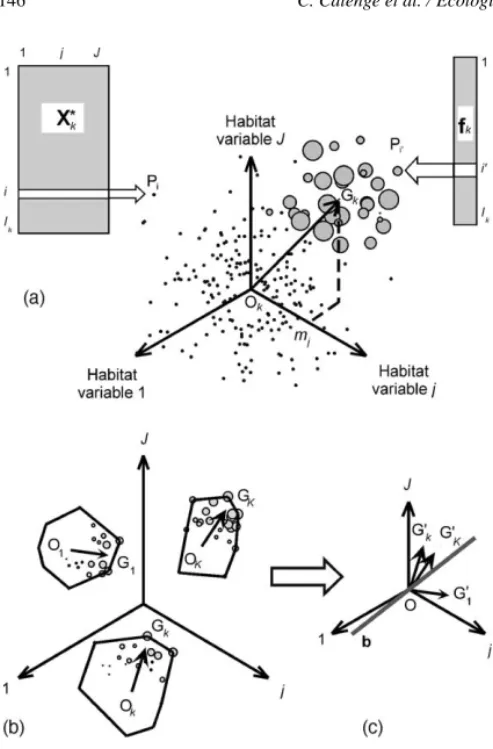
Fig. 1. Analysis of the marginality. (a) Case of one animal: the table X^∗_k, centered and standardized by columns, contains the values of J habitat variables on the Ikresource units available to the animal k. Each row of X^∗_k defines a point in the J-dimensional space of habitat variables. The origin Okof the space is located at the average of available habitat conditions. The vector fkcontains the relative frequencies of use of each unit by the animal. The diameter of the circles is proportional to these frequencies. The average mjof the habitat variable j is weighted by the relative frequencies of use. The mjs are the coordinates of the point Gk, which is located at the average used habitat conditions. The vector OkGkis the marginality vector of the animal k. (b) Case of K animals (design III): For each animal k, the average available habitat conditions define a point Okand the average used conditions define a point Gk. The vector OkGkis the marginality vector for animal k. (c) The K-select analysis proceeds in two steps:

first, a translation is applied to each vector OkGk, so that they all have a common origin O (the origin of space); second, an eigenanalysis is performed on the table of coordinates of the translated vectorsOGk

on habitat variables, so that the mean marginality projected on the first axis b is maximized.

2.2. The K-select analysis: a new method to analyse designs II and III data

In design III, the availability of habitat may vary from animal to animal, whereas it is the same for all ani-

mals in design II. Thus, a method developed for design III can also be used in design II studies, by setting all availabilities equal to the same value for each habitat variable. We therefore use here the above-described geometrical approach to build a multivariate analysis of the marginality for design III data, keeping in mind that the analysis can be extended to design II studies. We consider here a radio-tracking study of K animals. The RUs available to a given animal may be determined in different ways, e.g. all pixels located within a specified distance from an animal relocation. The global table X contains the value of the J habitat variables for all K animals:

X=





 X1

X₂ M X_K







This table has J columns and I rows, withI=_K

k=1I_k. Each table X_k is then transformed in X^•_k so that each column of the global table X^*:

X^∗=





 X^•₁ X^•₂ M X^•_K







is centered and has unit variance. For the animal k, the 1×J vector ak,

a_k=1 I_k1^t_I

kX^•_k

contains the coordinates of the mean of habitat condi- tions available to the animal k (Fig. 1b). Let f_kbe the I_k- dimensional vector that contains the proportion of the relocations of animal k numbered in each RU. Further, let u_k =f^T_kX^•_k. The vector 1×J u_kcontains the coordinates of the mean of habitat conditions used by animal k. Therefore, the vector m^•_k=u_k−a_kis the marginal- ity vector of animal k (seeFig. 1c). These vectors may be concatenated by row to form the K×J table M:

M=





 m^•₁ m^•₂ M m^•_K







(13)

The table M contains the coordinates of the K marginal- ity vectors on the J habitat variables. Let d_k be the proportion of all relocations collected for the animal k:

d_k = Ik

_K

k=1I_k

Let D_K=Diag(d1, . . . , d_k, . . . , d_K) be the weight matrix associated with the rows of the matrix M.

The animals thus have a weight proportionate to the number of their relocations. Note that under some cir- cumstances, the biologists may prefer to give uniform weights to all animals rather than weights proportionate to the number of their relocations. In this case, the animal weights are given by dk= 1/K instead of the above formula. The three matrices (M, IJ, DK) define a statistical triplet that can be analysed using an eige- nanalysis. That is, the K×J table M is to be analysed, the J×J identity matrix I_J defines the weights associated with the columns (square matrix with 1s on the diagonal and 0s elsewhere), and the K×K matrix D_K defines the weights associated with the rows. The total inertia of this analysis is equal to

Tr(M^TD_KMI_J)=^K

K=1

d_k||m^•_k||²,

i.e. equal to the mean marginality of the monitored animals, weighted by the number of relocations of each animal. Therefore, an eigenanalysis of the triplet (M, I_J, D_K) gives the linear combinations of habitat variables that maximize the mean marginality of the monitored animals on the first axes. On the resulting graphical display, the average of used habitat conditions is as far as possible from the average of available habitat conditions. This eigenanalysis is strictly equiv- alent to the non-centered PCA of the table M, with the uniform weighting for all columns and weights proportional to the number of animal relocations for the rows.

This analysis indicates the similarity of the habitat selection among several animals. When all the animals have the same habitat preferences, their marginality vectors are oriented in the same direction, and the first axes of the analysis explain a large part of the total inertia. Conversely, if the habitat selection differs from animal to animal, the component of the marginality explained by the first axes is not much larger than the inertia explained by the last.

An idea of the pertinence of this analysis can also be obtained using randomization tests. If we assume that the relocations are temporally independent, then under the null hypothesis of random habitat use, all the possible allocations of the_I_k

i=1vkirelocations of animal k in the RUs available to it are equiprobable.

“Random habitat use” marginality vectors can then be computed from this randomized data set, and a table M can be computed. This procedure is repeated several times and with each step, a K-select analysis is carried out and the first eigenvalue is stored. Finally, the first eigenvalue of the observed data set is compared to the distribution of the first eigenvalues of the randomized data sets. The tests presented in the case of design I data can also be applied to each individual using the Bonferroni correction (Bland and Altman, 1995; test of the marginality and test of the effects of variables on the marginality of each animal).

All these equations are given for the case of continuous variables, yet it is essential to note that this approach still holds for dummy (Tenenhaus and Young, 1985), fuzzy coded (Chevenet et al., 1994) or a mixture of quantitative and dummy variables (Hill and Smith, 1976). This analysis may therefore be used to analyse all kinds of habitat variables (categorical and/or continuous).

3. Application to wild boar (Sus scrofa L.) data 3.1. Description of the data

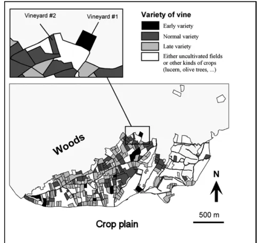
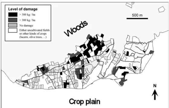
The procedure described above was applied to one data set concerning radio-tagged wild boars monitored in Pu´echabon, France (Maillard, 1996). The study area (4500 ha) is located in the south of France and the vegetation is typical of the Mediterranean habitat (gar- rigue dominated by Quercus ilex L.). The study area was mapped according to nine continuous variables:

elevation, slope, sunshine, distance from water, recreational trails and human areas, and density of herbaceous, shrubby and tree vegetation (Fig. 2). Two main topographical structures may be identified. The H´erault gorges pass through our study area and affect nearly all of our ecological variables. Indeed, this valley is characterized by low elevation, steep slopes, low sunshine, less dense herbaceous cover and is generally far from recreational trails. The Pu´echabon plateau, delimited

(14)

Fig. 2. Location and maps of the study area for wild boar radio-tracking at Pu´echabon, south of France. The studied variables are elevation, slope, sunshine, distance from recreational trails (Dtrails), distance from water (Dwater), density of vegetal cover (herbaceous, shrub and tree cover) and distance from crops (Dcrops).

by the gorges, is the core of our study area. Nine trap sites baited with maize were placed on this plateau in summer 1992 and 1993. Eleven wild boars were captured and fitted with radio collars. Animals were then relocated daily at their resting sites (Maillard, 1996).

We focus here on diurnal resting-site selection in summer (July–August). All of the pixels on the raster map located within 500 m from the relocations of a given animal were considered to be available to it, each pixel covering an area of one hectare. The habitat availability thus varied from one animal to another. We then applied the K-select analysis to this data. All analy-

ses were carried out using the R software (Ihaka and Gentleman, 1996).

3.2. Results

Habitat use appeared significantly non-random for nearly all animals, as indicated by the randomization tests carried out on the marginality vectors (Table 1a).

However, it is more difficult to learn from results of the tests carried out for each variable and each animal (Table 1b). These tests are rarely significant, even when the ␣-level is shifted to 0.1. Indeed, the

(15)

Table 1

Results of the randomization tests of habitat selection by the wild boar at Pu´echabon (design III data; see text)

WB1 WB2 WB3 WB4 WB5 WB6 WB7 WB8 WB9 WB10 WB11

(a) Tests of the marginality (Bonferroni␣level = 0.05/11 = 0.0045)

Marginality 1.058 2.600 3.057 1.499 0.452 2.280 0.634 1.089 1.145 2.412 2.452

# relocations 50 52 54 82 51 34 48 57 23 51 51

P-value 0.004 <0.0001 <0.0001 <0.0001 0.155 <0.0001 0.073 0.008 0.007 0.0003 0.0003 (b) Selection of habitat variables by each animal (Bonferroni␣level = 0.05/99 = 0.0005, two-tailed test)

Elevation 0.33 −0.93^* −0.94^* 0.37 −0.26 −0.55 −0.33 0.19 −0.27 −0.93^* −0.86^* Slope −0.69^* 0.39 0.26 0.05 0.02 0.48 −0.16 −0.17 −0.35 0.37 0.50 Sunshine 0.16 −0.45 −0.43 0.09 −0.09 −0.65^* 0.22 −0.16 −0.32 −0.56 −0.53 Trails −0.19 0.75â 1.17^* −0.14 0.21 0.72 0.27 0.07 −0.15 0.46 0.96^* Water 0.05 −0.64 −0.61 0.77â −0.06 −0.51 −0.36 0.29 −0.30 −0.60 −0.35 Herbaceous −0.35 −0.27 −0.30 0.34 −0.47 −0.45 −0.12 0.83â −0.51 −0.26 −0.19 Shrub −0.06 0.11 −0.14 0.78^* −0.02 −0.07 −0.13 0.2 0.44 0.03 0.22 Tree 0.53 0.56 0.20 0.12 −0.27 0.27 −0.29 0.39 −0.53 0.67 0.16

Crops 0.03 0.03 0.07 −0.14 0.18 0.53 −0.37 0.18 0.08 0.03 0.07

These tests are based on 10,000 randomization steps (NS: not significant). (a) significance of the marginality for each animal. (b) Coordinates of marginality vectors on habitat variable (i.e. the differences [mean used – mean available] for each wild boar and each variable). Using the mathematical notation presented in the text, this table corresponds to the table M^T (transpose of M). The column names correspond to the animals’ ID code.

a Significant at the 10% level.

∗Significant at the 5% level.

biggest drawback of the Bonferroni inequality is that it becomes even more conservative when a large number of tests are carried out (Bland and Altman, 1995, Faraway, 2002). In addition, habitat variables are cor- related among each other. It is therefore rather tricky to emphasize the important underlying factors from such tests. Finally, variation exists in habitat selection from animal to animal. For example, WB2 and WB3 exhibit similar habitat preferences, with selection of low ele- vations and selection of areas far from trails, whereas WB1 selects the steep slopes. Because of this variation of preferences, it is difficult to summarize the patterns of habitat selection from only these results.

This individual variability in habitat selection should not be ignored (Mysterud and Ims, 1998) and the K-select analysis may be used to summarize the patterns of habitat choice. The first eigenvalueλ1of the analysis is larger than what is expected under the random habitat use hypothesis (λ1= 1.203, P < 0.0001).

In other words, the K-select analysis is pertinent, and there is at least one group of several animals all display- ing some similarity in habitat preferences. Since this method is a PCA-like analysis, the results should be analysed in the same manner. The barplot of eigenvalues indicates the amounts of marginality explained by each factorial axis (Fig. 3a). The amount of explained

marginality decreases regularly after the second axis, indicating that the following axes account for “random noise”. We thus analysed the marginality on the first two axes, keeping in mind that the first axis explained a larger part of the marginality than the second.

The biological interpretation of the axes is done according to the variable loadings (Fig. 3b). The first axis was explained by an opposition between the Hérault gorges (close to water and far from recreational trails, with low elevation, higher slopes and low sunshine) and the Puéchabon Plateau (further from water and closer to trails, with high elevation, low slopes and high sunshine). The second axis is mainly explained by the density of vegetation cover (herbaceous, shrub and tree cover). Three main groups of animals may be identified (Fig. 3c). A first group strongly selected the Hérault gorges for their resting site (WB11, WB10, WB2, WB6 and WB3). Animals of the second group preferred the plateau (WB4 and WB8), but also strongly selected a dense vegetation cover for their resting sites. The third group of animals included the boars (WB1, WB9, WB7 and WB5) with a weaker or even non-significant marginality (Table 1a).

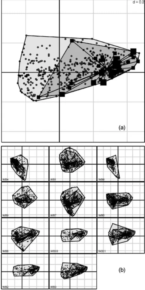
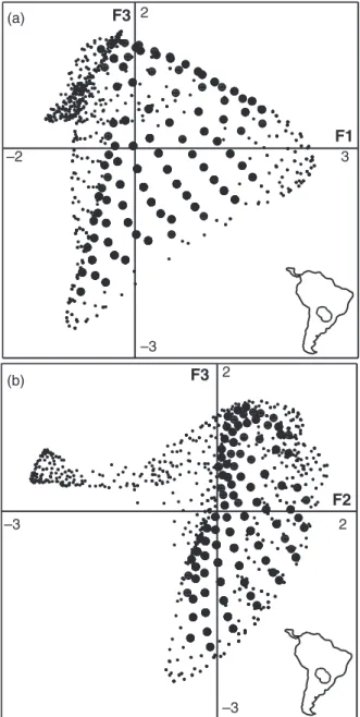
A graphical display of the niche of a given animal is obtained by projecting the cloud of available pixels on the first two factorial axes (Fig. 4). This is done by

(16)

Fig. 3. Results of the K-select analysis carried out to highlight habitat selection by 11 wild boars on nine habitat variables: (a) bar chart of the eigenvalues, measuring the mean marginality explained by each factorial axis; (b) variable loadings on the first two factorial axes; (c) projection of the marginality vectors of all animals on the first factorial plane. All marginality vectors are recentered such that habitat availability is the same for all animals (common origin to all vectors).

projecting the matrix X^*onto the axes of the analysis.

The origin of this graph is the barycenter of the pixels available to all animals, since X^*is centered by column.

We then add black squares with areas proportional to the number of relocations counted in the pixels. A star connecting all used pixels identifies the animal niche in the space of available resources. Finally, the contour polygon of available pixels (light grey in Fig. 4) and of used pixels (dark grey) completes the representation of the niche of the animal. The position of the available pixels relative to the origin gives an idea about the accessibility of the main characteristics highlighted by the analysis to a given animal.

The difference in habitat selection between the three groups may thus be explained by the difference in habitat availability for the animals (“functional responses”, Mysterud and Ims, 1998). Most animals select the

Fig. 4. Representation of the niche of the wild boars monitored at Pu´echabon on the first two factorial axes. (a) Detail for wild boar

#3, (b) The same graphical display for all monitored animals. Note that the graphs are ordered according to the coordinates of the corresponding animals on the first factorial axis (negative values are at the upper left hand corner and positive values at the lower right hand corner).

gorges, a favorable place for resting. The absence of recreational trails and the steep slopes encountered in this area ensure the absence of human disturbance, while the lower sunshine occurring in the gorges is

(17)

certainly a key factor in their selection, especially dur- ing summer, in the warm Mediterranean environment.

The gorges were very accessible for this group of animals. Moreover, the second group (WB4 and WB8) had greater limitations in access to these areas (Fig. 4).

Their home range was indeed located on the Plateau.

Thus, they selected the densest vegetation areas for their resting sites, probably to limit human disturbance.

We stress that these conclusions are only valid for the scale of the study (Johnson, 1980). Availability as defined in this example can also measure habitat use in studies carried out on a larger spatial scale. For example, all the pixels on the raster map located within 500 m from a relocation could be used to characterize the selection of the home range within the study area. If the habitat selection was studied on a larger scale, these pixels could have been considered as used, and availabilities could have been set equal to the composition of the study area. In this case, the K-select analysis might have helped to identify the most important factors in the selection of home range within the study area. The K-select analysis can therefore be used for data analysis in multi-scale analysis of habitat selection.

4. Discussion

A new method is developed to point out the habitat selected by a species in designs II and III studies. The K-select analysis led us to identify the main features of the habitat selected by the wild boar for its resting site in a Mediterranean environment. We thus detected a functional response in habitat selection, i.e. a variation of the habitat selection according to the habitat availability which we used to build a typology of the animals. This analysis is therefore suitable when the objective is to define one or several groups of animals that select the same habitat characteristics.

Wildlife habitat studies generally use other kinds of eigenanalyses, such as principal component analysis or multiple correspondence analysis. This is viewed as a preliminary step to reduce the number of variables before further predictive analyses (e.g.Brown and Batzli, 1984on the squirrel;Abaigar et al., 1994on the wild boar). This strategy has been severely criticized, however, because there is no indication that the first factorial axes are those of interest to the focus species, even if they account for most of the spatial variability

in the study area. As noted byJohnson (1981), “there is no reason to assume that a principal component necessarily relates to the animal or its needs. The animal could be responding to one of the variables that is a minor component of all that were measured”.

The K-select analysis focuses on the differences between habitat use and availability. This approach consists of a PCA performed on a non-centered table.

As stated byNoy-Meir (1973), “mathematically and geometrically, centering involves the specification of the origin (. . .). It is the ‘point of zero information’;

anything that is at it, is trivial and uninteresting; anything that deviates from it is information”. Thus, by considering the average available habitat conditions as the origin of ecological space, an eigenanalysis of the table containing the relative position of the average used habitat conditions finds the linear combination of habitat variables for the habitat selection which is the largest. These synthesis variables are of strong ecological interest for the stated objectives, especially for the identification of the habitat variables selected by animals.

This analysis is neither restricted by the number of habitat variables nor by the number of animals, which is another very attractive characteristic of the method.

A strong correlation among habitat variables has no negative effect on the results. Even a small number of animals allows for the description of the relationships between habitat use and availability. It can limit, however, the biological conclusions drawn from the analysis and therefore influence the inferential power of the technique.

The K-select analysis focuses on only one parameter of the niche, the marginality. This criterion measures the squared distance between the optimum for an animal and the average available habitat conditions. Actu- ally, another parameter which could be of interest to biologists is the tolerance (Dol´edec et al., 2000; Hirzel et al., 2002), i.e. the variance of habitat use around this optimum on habitat variables. It is worth noting two points here, however: (i) performing the randomization tests on marginality vectors is equivalent to testing the importance of the marginality relative to the tolerance for each animal: the test is significant when the marginality is large relative to the tolerance; (ii) the K- select analysis focuses on the “between-animal” variability, not on the “within-animal” variability. Indeed, in habitat selection studies relying on radio-tracking

(18)

data, the sampling unit of interest is often the animal and rarely the relocation (Aebischer et al., 1993; Otis and White, 1999).

The application of the K-select analysis only requires that the relocations of the animals are independent and representative of the actual habitat use of the animals. The sensitivity of the analysis to temporal autocorrelation between the relocations merits further investigation. Temporal autocorrelation occurs when the time interval between two relocations is short, because, in that case, the position of a relocation depends on the position of the previous one (Swihart and Slade, 1985). The K-select analysis in itself is not affected by autocorrelation, as this analysis is mainly exploratory. However, when this hypothesis is violated, the randomization tests of the marginality vectors are not valid since all permutations of the frequencies of use in the available resource units are not equiprobable.

In other words, when autocorrelation is present in the data, one works with trajectories of the animals, and no longer with a random sample of relocations. This point needs to be taken into account in the randomization tests. For example, Martin (2004) recommends gen- erating random walks with the same properties as the observed trajectories (same distance between successive relocations). The simulated data can then be used as an estimation of random habitat use in the randomization tests, instead of a random sample of independent points.

Here, we have provided a powerful tool to identify, among a set of habitat variables, those that are of interest in resource selection studies based on designs II and III data. With the development of new tech- nologies such as GIS or GPS, biologists who formerly had meager data sets now have to deal with too much data. Among all the variables potentially useful to describe the habitat of a species, only a limited number should be used for prediction of habitat use (Boyce and McDonald, 1999). For this reason, the first axes of a K- select analysis could be included in a predictive model of habitat use. We stress that this perspective merits further investigation.

5. Software availability

This analysis, as well as other computational tools, is available in the “adehabitat” package for R software

(Ihaka and Gentleman, 1996), and can be downloaded for free at the URLhttp://cran.r-project.org/.

Acknowledgements

We are grateful to the Office national de la chasse et de la faune sauvage for their financial support. We warmly thank Daniel Chessel (University of Lyon, France), for his help in the development of the K- select analysis, and Jean-Michel Gaillard (University of Lyon, France), for his invaluable comments on ear- lier drafts of this paper.

References

Abaigar, T., Del Barrio, G., Vericad, J.R., 1994. Habitat preference of wild boar (Sus scrofa L., 1758) in a Mediterranean environment.

Indirect evaluation by signs. Mammalia 58, 201–210.

Aebischer, N.J., Robertson, P.A., Kenward, R.E., 1993. Composi- tional analysis of habitat use from animal radio-tracking data.

Ecology 74, 1313–1325.

Bland, J.M., Altman, D.G., 1995. Multiple significance tests: the Bonferroni method. Br. Med. J 310, 170.

Boyce, M.S., McDonald, L.L., 1999. Relating populations to habitats using resource selection functions. Trend. Ecol. Evol. 14, 268–272.

Brown, B.W., Batzli, G.O., 1989. Habitat selection by fox and gray squirrels: a multivariate analysis. J. Wildl. Manage. 48, 616–621.

Burnham, K.P., Anderson, D.R., 1998. Model selection and infer- ence. In: A Practical Information-theoretic Approach. Springer Verlag, Berlin, Germany.

Chevenet, F., Doledec, S., Chessel, D., 1994. A fuzzy coding approach for the analysis of long-term ecological data. Fresh- water Biol. 31, 295–309.

Dol´edec, S., Chessel, D., Gimaret-Carpentier, C., 2000. Niche sep- aration in community analysis: a new method. Ecology 81, 2914–2927.

Erickson, W.P., Mc Donald, T.L., Skinner, R., 1998. Habitat selection using GIS data: a case study. J. Agric. Biol. Environ. Stat. 3, 280–295.

Escoufier, Y., 1987. The duality diagram: a means of better practical applications. In: Legendre, P., Legendre, L. (Eds.), Develop- ment in Numerical Ecology, NATO Advanced Institute, Series G. Springer Verlag, Berlin, pp. 139–156.

Faraway, J.J., 2002. Practical Regression and ANOVA using R.

Department of Statistics, University of Michigan, USA.

Guisan, A., Zimmermann, N.E., 2000. Predictive habitat distribution models in ecology. Ecol. Model 135, 147–186.

Guisan, A., Edwards, T.C., Hastie, T., 2002. Generalized linear and generalized additive models in studies of species distributions:

setting the scene. Ecol. Model 157, 89–100.

(19)

Hall, L.S., Krausman, P.R., Morrison, M.L., 1997. The habitat concept and a plea for standard terminology. Wildl. Soc. Bull. 25, 173–182.

Hausser, J., 1995. S¨augetiere der Schweiz. Mammif`eres de la Suisse.

In: Mammiferi della Svizzera. Birkh¨auser Verlag, Berlin, Ger- many.

Hill, M.O., Smith, A.J.E., 1976. Principal component analysis of taxonomic data with multi-state discrete character. Taxon 25, 249–255.

Hirzel, A.H., Hausser, J., Chessel, D., Perrin, N., 2002. Ecological- niche factor analysis: How to compute habitat-suitability maps without absence data? Ecology 83, 2027–2036.

Hutchinson, G.E., 1957. Concluding remarks. Cold Spring Harbor Symp. Quantitat. Biol. 22, 415–427.

Ihaka, R., Gentleman, R., 1996. R: A language for data analysis and graphics. J. Comput. Graphic. Stat. 5, 299–314.

Johnson, D.H., 1981. The use and misuse of statistics in wildlife habitat studies. In: Capen, D.E. (Ed.), The use of Multivariate Statistics in Studies of Wildlife Habitat, U.S. Fish and Wildlife Service. USDA Forest Service, pp. 11–19.

Johnson, D.H., 1980. The comparison of usage and availability measurements for evaluating resource preference. Ecology 61, 65–71.

Knick, S.T., Dyer, D.L., 1997. Distribution of black-tailed jackrab- bit habitat determined by GIS in southwestern Idaho. J. Wildl.

Manage. 61, 75–85.

Maillard, D., 1996. Occupation et utilisation de la garrigue et du vignoble m´editerran´eens par le Sanglier. Thesis. University of Aix-Marseille III, Marseille, France.

Manly, B.F.J., 1994. Multivariate Statistical Methods. A primer, 2nd ed. Chapman & Hall, London, UK.

Manly, B.F.J., 1997. Randomization, Bootstrap and Monte Carlo Methods in Biology, 2nd ed. Chapman & Hall, London, UK.

Manly, B.F.J., McDonald, L.L., Thomas, D.L., McDonald, T.L., Erickson, W.P., 2002. Resource Selection by Animals: Statistical Design and Analysis for Field Studies, 2nd ed. Kluwer Academic Publishers, Dordrecht, The Netherlands.

Martin, J., 2004. Importance des structures spatiales et des con- traintes comportementales dans les études de sélection de l’habitat. Msc Thesis, Université Claude Bernard Lyon 1, Lyon.

Morrison, M.L., Marcot, B.G., Mannan, R.W., 1992. Wildlife–

Habitat Relationships. Concepts and Applications. The Univer- sity of Wisconsin Press, Madison, WI.

Morrison, M.L., 2001. A proposed research emphasis to overcome the limits of wildlife-habitat relationship studies. J. Wildl. Man- age. 65, 613–623.

Mysterud, A., Ims, R.A., 1998. Functional responses in habitat use:

availability influences relative use in trade-off situations. Ecology 79, 1435–1441.

Noy-Meir, I., 1973. Data transformation in ecological ordination. I.

Some advantages of non-centering. J. Ecol. 61, 329–341.

Otis, D.L., White, G.C., 1999. Autocorrelation of location estimates and the analysis of radiotracking data. J. Wildl. Manage. 63, 1039–1044.

Schooley, R.L., 1994. Annual variation in habitat selection: patterns concealed by pooled data. J. Wildl. Manage. 58, 367–

374.

Swihart, R.K., Slade, N.A., 1985. Testing for independence of observations in animal movements. Ecology 66, 1176–1184.

Tenenhaus, M., Young, F.W., 1985. An analysis and synthesis of multiple correspondence analysis, optimal scaling, dual scaling, homogeneity analysis and other methods for quantifying categorical multivariate data. Psychometrika 50, 91–119.

Thomas, D.L., Taylor, E.J., 1990. Study designs and tests for com- paring resource use and availability. J. Wildl. Manage. 54, 322–

330.

(20)

(21)

(22)

(23)

1 Running head: FACTORIAL ANALYSIS OF SELECTION RATIOS

1 2

FACTORIAL ANALYSIS OF SELECTION RATIOS FROM ANIMAL 3

RADIO-TRACKING DATA 4

5

C. CALENGE,^1,2AND A.B. DUFOUR ¹