Actuator and sensor design and modeling for structural acoustic control

Actuator and Sensor Design and Modeling for Structural Acoustic

Control

by

Robert Jeffrey Pascal

B.S., Aerospace Engineering The University of Texas at Austin, 1994

SUBMITTED TO THE DEPARTMENT OF AERONAUTICS AND ASTRONAUTICS IN PARTIAL FULFILLMENT OF THE DEGREE OF

MASTER OF SCIENCE IN AERONAUTICS AND ASTRONAUTICS

AT THE

MASSACHUSETTS INSTITUTE OF TECHNOLOGY

MAY 1999

© 1999 Massachusetts Institute of Technology All rights reserved

Signature of Author ... Department of Aeroiautics

A

\ 1 b Thesis Supervisor

Jaime Peraire Professor of Aeronautics and Astronautics Chairman, Department Graduate Committee

F U

Mr*V1

,i1

1

5

1999

Actuator and Sensor Design and Modeling for Structural Acoustic

Control

by

ROBERT JEFFREY PASCAL

Submitted to the Department of Aeronautics and Astronautics on May 21, 1999 in Partial Fulfillment of the

Requirements for the Degree of Master of Science at the Massachusetts Institute of Technology

ABSTRACT

The use of a high-fidelity finite element model is investigated for the design and closed-loop performance prediction of shaped and distributed sensors and actuators for structural acoustic control. Sensor and actuator design was found to be sensitive to nodeline dis-crepancies between the model and experiment caused by moderate manufacturing defects and/or boundary condition uncertainties. Relying on the finite element model for sensor shaping or distribution results in a slight difference between the desired and achieved sen-sor performance. The modeshape sensitivity is compounded when both the actuator and sensor are shaped or distributed, as is the case with a distributed sensuator design. This results in an unacceptable difference between the desired and achieved distributed sensua-tor performance. Since the advantages of shaping and distribution can be gained either at the system input (actuators) or output (sensors), modeshape information from a correlated analytic model should be used for one or the other, but not both. Experimental verification of critical modeshapes is also recommended to reduce sensor and actuator performance loss.

The finite element model was also used to predict achievable closed-loop acoustic perfor-mance for various sensor and actuator pairs for transmission and reflection control. Since a finite element model is generally not accurate enough to be used as the basis for high performance compensator design, the predicted performance was compared to experimen-tal results of compensators designed with an accurate data-fit model using the same con-trol design methods. Good correlation was achieved between predicted and implemented results for linear behavior of the system.

Finally, a comparison was made between a modally shaped PVDF sensor/PZT actuator design and a single wafer PZT sensuator. Both have desirable open-loop characteristics and comparable predicted performance. The predicted performance could not be imple-mented for the sensuator design due to a severe amplitude non-linearity. The PVDF sen-sor design is very linear, and the implemented performance slightly exceeded that predicted using the finite element model. Due to the implementation difficulties of the

4 ABSTRACT

sensuator, the PVDF sensor/PZT actuator design is the better choice for acoustic transmis-sion control.

Thesis Supervisor:

Professor David W. Miller

ACKNOWLEDGMENTS

Funding for this research was provided by the U.S. Air Force Office of Scientific Research (AFOSR), under AASERT Grant No. F49620-97-1-0358 (Parent Grant No. F49620-96-1-0290) with Capt. Brian Sanders as the AFOSR contract monitor, Charlotte Morse as the MIT senior contract administrator, SharonLeah Brown as the MIT fiscal officer, and Karen Buck as the AFOSR contract administrator.

Continuous guidance for the research was provided by Professor David Miller. The foun-dation for this research was laid by Dr. Roger Glaese, who was always eager to offer detailed explanations of his work. Much of this research occurred in parallel with the work of Koji Asari, whose advice and support is greatly appreciated. Collaboration with Dr. Steve Griffin of AFRL during a January 1998 visit proved to be an extremely valuable experience, as well as the basis for continued interaction. Dr. Carl Blaurock of Mide Technology Corporation was consulted on many occasions for his knowledge of shaped PVDF sensors. Carlos Gutierrez assisted with and is continuing the work on the active membrane. Last but not least, the sensuator work could not have been accomplished with-out the electronics expertise and patience of Paul Bauer.

TABLE OF CONTENTS

1.2.1 Passive Structural Redesign 1.2.2 Active Transmission Contro 1.3 Reflection Control ... 1.3.1 Passive Acoustic Damping 1.3.2 Active Reflection Control 1.4 Approach for Current Research 1.4.1 Experimental Description 1.4.2 Thesis Outline ... Chapter 2. Finite Element Modeling 2.1 Discussion of Model Fidelity and L 2.2 Structural Acoustic Modeling in Al 2.3 Modal State Space Approach .. 2.4 Sensor and Actuator Modeling 2.4.1 Microphones ... 2.4.2 Accelerometers ... 2.4.3 Strain Gages ... 2.4.4 Speakers ... 2.4.5 Piezoelectric Sensors and A 2.5 Open-Loop Model Correlation . . . . . 19 . . . 20 . . . . . 20 1 . . . . 2 2 . . . 2 3 . . . 2 3 . . . . . 24 . . . 2 5 . . . . . 2 5 . . . .. . . .. 27 . . . . . 2 9 Jses .. . . .. . 29 N SY S . . . 31 . . . . 34 . . . . 36 . . . . 37 . . . . 3 8 . . . . 39 . . . . 4 1 ctuators . . . 43 . . . . . 4 6 Abstract Acknowledgments Table of Contents List of Figures .. . List of Tables . . . Nomenclature ... Chapter 1. Introduction 1.1 Motivation ... 1.2 Transmission Control

8 TABLE OF CONTENTS

2.5.1 Control to Feedback Transfer Functions .

2.5.2 Disturbance to Feedback Transfer Functions

2.5.3 Control to Performance Transfer Functions 2.5.4 Disturbance to Performance Transfer Functions

2.6 Summary . . . . . . . .. 5 3 Chapter 3. Sensor and Actuator Design ....

3.1 Modally Shaped PVDF Sensor . . . . 3.1.1 Modal Observability and Rolloff 3.1.2 Sensitivity to Predicted Modeshape 3.2 Piezoelectric Sensuator Design . . . .

3.2.1 Single Wafer PZT Sensuator on Plate 3.2.2 Distributed PZT Sensuator on Plate 3.3 Summary

Chapter 4. Predicted Compensator Performance . ... 79

4.1 Transmission Compensators ... 80

4.1.1 ShapedPVDF Sensor ... 80

4.1.2 Single PZT Sensuator ... 81

4.1.3 Distributed PZT Sensuator ... .... 82

4.1.4 FEM Based Compensator ... 83

4.2 Reflection Compensator ... 85

4.3 Summ ary ... ... 87

Chapter 5. Experimental Validation ... .... 89

5.1 Transmission Compensators ... 89

5.1.1 ShapedPVDF Sensor ... 90

5.1.2 Single PZT Sensuator ... 91

5.1.3 FEM Based Compensator ... ... .. 96

5.2 Reflection Compensator ... ... . 96

5.3 Comparison of Predicted vs. Experimental Performance . ... 98

5.4 Comparison of Shaped PVDF Sensor vs. PZT Sensuator . ... 99

Chapter 6. Conclusions ... . 101

6.1 Summ ary ... 101

TABLE OF CONTENTS 9

References .. ... .... ... 105

Appendix A. Finite Element Model Modeshapes ... 109

A. 1 Uncoupled Modeshapes ... 109

A.1.1 Structural ... ... 110

A .1.2 A coustic . . . . . . .. . . 114

A.2 Coupled Modeshapes ... ... . 117

A .2.1 Structural ... .. . ... .. . .... 118

A .2.2 A coustic . . . . . . .. . . 122

Appendix B. Investigation of Circulance . ... .. 127

Appendix C. Active Membrane for Reflection Control . ... 131

C. 1 Response of Membrane to Acoustic Excitation . ... 131

C.2 M embrane Actuation ... 133

LIST OF FIGURES

Figure 1.1 Diagram of acoustic test chamber configuration. . ... 26 Figure 1.2 Diagram of open chamber configuration used for structural identification

and initial sensor/actuator testing. . ... . 27 Figure 2.1 ANSYS mesh of chamber finite element model with wedge cutaway from

acoustic elements to expose structural components. . ... 32 Figure 2.2 Block diagram of input/output characteristics of finite element model. 37 Figure 2.3 Sketch of nodal locations and coordinate directions for bi-cubic

inter-polation of FEM results ... 41

Figure 2.4 Edge moment actuation of PZT wafer. . ... 44 Figure 2.5 Finite element model to data correlation transfer functions for control

input to various feedback sensors. . ... . 48 Figure 2.6 Finite element model to data correlation transfer functions for disturbance

input to various feedback sensors. . ... . 49 Figure 2.7 Finite element model to data correlation transfer functions for control

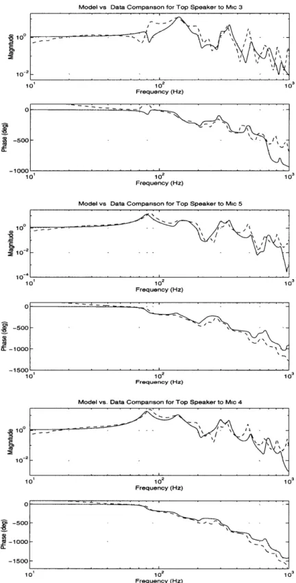
input to performance microphones. . ... 51 Figure 2.8 Finite element model to data correlation transfer functions for disturbance

input to performance microphones. ... . ... . 52 Figure 3.1 Slope nodelines of the second and third symmetric plate modes used for

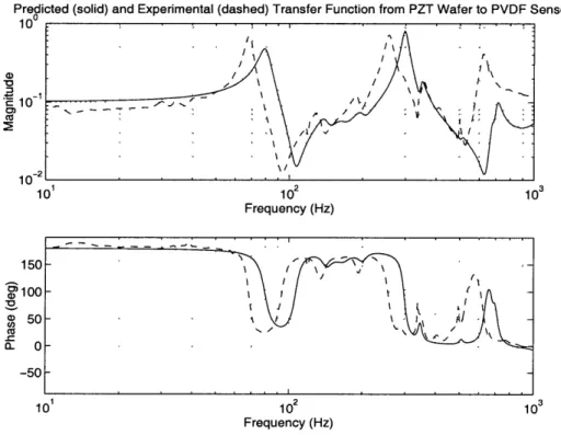
design of a modally shaped PVDF strain sensor. ... 57 Figure 3.2 Comparison of predicted and experimental transfer function from PZT

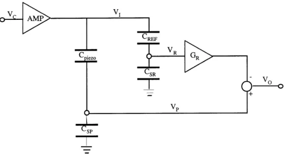
wafer to modally shaped PVDF strain sensor. . ... . 58 Figure 3.3 Simple piezoelectric sensuator circuit for simultaneous actuation and

sensing of structural vibration. . ... .. 59 Figure 3.4 Detailed schematic of single wafer PZT sensuator circuit. ... . 60 Figure 3.5 Photograph of single PZT sensuator circuit on protoboard. ... 61 Figure 3.6 Experimental and finite element model single PZT sensuator transfer

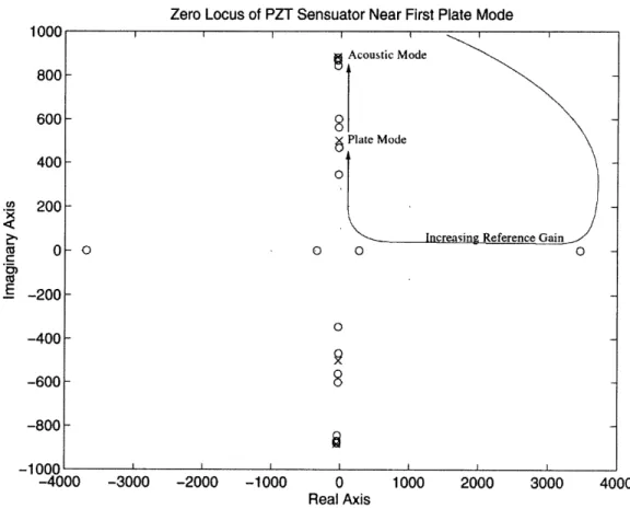
functions for various circuit tunings . ... 63 Figure 3.7 Zero locus of single wafer PZT sensuator near first plate mode. ... 64 Figure 3.8 Positive real transfer functions for single wafer PZT sensuator. .... 67 Figure 3.9 Slope nodelines for first two symmetric modes of clamped-clamped beam

12 LIST OF FIGURES

Figure 3.10 Predicted sensuator transfer function from finite element model using four symmetrically distributed PZT wafers. . ... 70 Figure 3.11 Magnitude and phase variation of electrical admittance of distributed

sensuator PZT wafers vs. frequency. . ... 72 Figure 3.12 Detailed schematic of distributed sensuator circuit. . ... . . 73 Figure 3.13 Photograph of distributed sensuator wafers bonded to plate. ... 74 Figure 3.14 Experimental transfer function for distributed PZT sensuator in open

chamber configuration. ... 75

Figure 3.15 Transfer function from distributed PZT wafers to collocated PVDF

sensors in open chamber configuration. . ... 76 Figure 4.1 Predicted performance of LQG transmission compensator from

distur-bance speaker to PVDF sensor and RSS pressure. . ... . . 81 Figure 4.2 Predicted performance of LQG transmission compensator from

distur-bance speaker to single wafer PZT sensuator and RSS pressure. ... 83 Figure 4.3 Predicted performance of LQG transmission compensator from

distur-bance speaker to distributed PZT sensuator and RSS pressure. ... 84 Figure 4.4 Predicted performance of FEM based LQG transmission compensator

from disturbance speaker to accelerometer and RSS pressure. ... 85 Figure 4.5 Predicted performance of MIMO LQG transmission and reflection

compensator from disturbance speaker to RSS pressure. . ... 86 Figure 5.1 Comparison of data-fit model to data for single wafer PZT sensuator

transfer function. ... 90

Figure 5.2 Implemented and predicted performance of LQG transmission compen-sator from disturbance speaker to PVDF sensor and RSS pressure. . . 91 Figure 5.3 Predicted performance of LQG transmission compensator from

distur-bance speaker to sensuator and RSS pressure convolved with data and using finite element model. ... 92 Figure 5.4 Implemented performance of LQG transmission compensator from

disturbance speaker to sensuator and RSS pressure. . ... 93 Figure 5.5 Nichols plots of loop transfer function showing sensuator amplitude

nonlinearity and resulting closed-loop instability. . ... . . 94 Figure 5.6 Implemented LQG compensator using single wafer PZT wafer manually

adjusted for maximum broadband acoustic performance. . ... . 95 Figure 5.7 Implemented and predicted performance of LQG finite element model

based transmission compensator from disturbance speaker to

LIST OF FIGURES 13

Figure 5.8 Implemented and predicted performance of LQG transmission and reflection compensator from disturbance speaker to RSS pressure using successive loop closure. ... 97 Figure A. 1 Plate axisymmetric modes for uncoupled finite element model. .... 110 Figure A.2 Plate asymmetric modes for uncoupled finite element model. ... .111 Figure A.3 Lower chamber longitudinal acoustic modes for uncoupled finite

element model. ... 114

Figure A.4 Lower chamber transverse acoustic modes for uncoupled finite element

model ... ... 115

Figure A.5 Upper chamber acoustic modes for uncoupled finite element model. . 117 Figure A.6 Bottom and top chamber speaker modes for coupled finite element

model. ... ... 118

Figure A.7 Plate axisymmetric modes for coupled finite element model. ... 118 Figure A.8 Plate asymmetric modes for coupled finite element model. ... 119 Figure A.9 Lower chamber longitudinal acoustic modes for coupled finite element

model ... ... 122

Figure A. 10 Lower chamber transverse acoustic modes for coupled finite element

m odel . . . 123 Figure A.11 Upper chamber acoustic modes for coupled finite element model. . . . 125 Figure C. 1 Transfer functions from bottom speaker to membrane acceleration and

microphones with and without membrane dividing chamber. ... 132 Figure C.2 PVDF actuator on inflated Mylar membrane with plywood spacer in

open chamber configuration. ... 134 Figure C.3 Transfer functions from PVDF actuator to accelerometer and PVDF

sensor for differential pressures between the membrane and aluminum plate. . . . .. 135 Figure D. 1 Wave model of SDOF oscillator dividing reverberant acoustic enclosure

LIST OF TABLES

Effect of structural redesign on acoustic transmission ... 21

Survey of active structural acoustic transmission control research . . . 23

Modal damping ratios for finite element model . ... 34

Physical parameters of speaker ... .. 42

Constants used for modeling PZT wafer on aluminum plate ... 45

Open loop correlation between finite element model and data ... 47

Numerical solution of zero migration in infinite order model as function of sensuator tuning parameter ... 65

Performance comparison between FEM prediction and implementation 99 Comparison of theoretical and measured acoustic frequencies with and without membrane ... 133

Change in acceleration and PVDF signal with differential pressure . . 135

NOMENCLATURE

Matrix of top speaker Matrix of bottom speaker Matrix of plate

Matrix of top acoustic chamber Matrix of bottom acoustic chamber Matrix in modal coordinates

Matrix of uncoupled, mass normalized modeshapes Density of air

Poisson's ratio

Diagonal matrix of natural frequencies Modal damping ratios

FEM fluid-structure coupling matrix in physical coordinates State space system, input, output, and feedthrough matrices Wave propagation speed

Blocked capacitance of PZT sensuator Reference capacitor in sensuator circuit

Charge sensor capacitors for piezo and reference leg of sensuator circuit Piezoelectric strain coefficient in x-direction for electric field in z-direction Young's modulus

Tuning gain for sensuator circuit

FEM stiffness matrix in physical coordinates FEM mass matrix in physical coordinates

Pressure degrees of freedom in physical coordinates

Structural and pressure degrees of freedom in modal coordinates State space input vector

Out-of-plane structural displacement

Structural degrees of freedom in physical coordinates (x, y, z, Rx, Ry, Rz) State space output vector

Chapter 1

INTRODUCTION

1.1 Motivation

Vibro-acoustic loads during launch are by far the most severe vibration environment a payload experiences during its service life. This loading condition is often the design load for much of the payload structure. Significantly reducing this environment could result in lighter payload structures, and/or reduced spacecraft failures. Passive methods such as mass loading and acoustic blankets are currently used to reduce the acoustic environment inside a payload fairing; however, recent research has focused on active methods which hold promise for much greater acoustic attenuation. [Leo & Anderson, 1996]

As with any active control method, the achievable performance is closely linked to the choice of sensors and actuators. The type, shape, and distribution of sensors and actuators with respect to the dynamics of the structure determine the characteristics of the transfer functions ultimately used in a closed-loop control system. Careful design of the sensors and actuators can lead to very favorable transfer function attributes such as modal filtering, rolloff, and bounded phase over a frequency region. The best sensor and actuator design for achieving these attributes requires very accurate knowledge of the coupled

structural-acoustic dynamics.

Several modeling methods are currently used to predict response of a structural-acoustic system. These include Statistical Energy Analysis (SEA), data identification models,

20 INTRODUCTION

wave models, and finite element models. Only the latter two are appropriate for sensor and actuator design since they retain the physics of individual dynamic modes; however, these models are not very accurate unless correlated extensively with experimental data. The finite element method is widely used because it offers the flexibility required for model correlation. The motivation for this thesis is to better define the capabilities and limitations of a correlated finite element model for sensor and actuator design. Addition-ally, the prediction of closed-loop performance using a sensor/actuator pair is motivated by its obvious value to the design process.

1.2 Transmission Control

Vibro-acoustic energy from the launch vehicle engines must follow one of the following transmission paths in order to enter the payload fairing. The first is the direct structural load path supporting the fairing and payload. Energy traveling this path vibrates both the fairing and payload, both of which excite the enclosed acoustic field. The second path is acoustic transmission, where acoustic energy from the external field vibrates the payload fairing which then excites the enclosed acoustic field. This second path is the focus of transmission control for this research.

1.2.1 Passive Structural Redesign

The first option that should always be considered when solving a structural-acoustic or vibration control problem is passive structural redesign. For the acoustic transmission problem, this includes the effect of varying the structural mass and stiffness, or adding passive structural damping treatments. For this investigation, a wave model of a single degree of freedom oscillator (simple structural model) dividing a non-reverberant acoustic far-field (external acoustic field) from a reverberant acoustic enclosure (fairing) was used. This model is developed in Appendix D. The structural and acoustic parameters were set to be similar to the acoustic test chamber used in this research. The disturbance source for this model is an incoming acoustic wave in the non-reverberant far field.

Transmission Control 21

Table 1.1 shows the acoustic performance improvements due to varying the structural parameters in the model. The performance was evaluated as the root sum square of five equally spaced pressure locations in the acoustic enclosure over a frequency range of 10Hz - lkHz. The nominal performance is for 1% structural and 1% acoustic damping ratios.

TABLE 1.1 Effect of structural redesign on acoustic transmission

Structural Variation Performance Improvement

5% Damping 0.92 dB

10% Mass Increase 0.70 dB

10% Mass Decrease -0.81 dB

10% Stiffness Increase -0.03 dB 10% Stiffness Decrease 0.004 dB

Increasing the structural damping or mass is seen to have a moderate effect on the perfor-mance. The performance is fairly insensitive to variations in structural stiffness. These performance trends are dependent on the acoustic resonances being at higher frequency than the fundamental structural mode. Adding mass causes attenuation at frequencies above the structural resonance, damping causes attenuation at the resonance, and stiffness causes attenuation below the structural resonance. Since almost all of the acoustic energy is at or above the structural resonance, adding structural mass or damping are the two pri-mary passive options. Addition of non-structural mass is the most common form of pas-sive structural redesign currently used to reduce acoustic transmission in payload fairings.

[Leo & Anderson, 1996]

Another trend seen in Table 1.1 is that both increasing stiffness and decreasing mass cause an increase in the acoustic energy transmitted into the enclosure. This combination is sim-ilar to the effect of changing from a built-up aluminum to a composite fairing design. In addition, composite structures tend to have less damping than built-up metal ones. This

22 INTRODUCTION

simple model therefore captures the trend that composite fairing designs generally exhibit which makes the enclosed acoustic environment more severe. [Denoyer, et al., 1998]

1.2.2 Active Transmission Control

The performance improvement achievable through passive means is only moderate, and for the case of composite fairings may only return the acoustic environment to the levels expected for a built-up aluminum fairing. The high launch cost per pound also presents practical limits on the use of added mass or passive damping treatments, and motivates the investigation of active control techniques for acoustic transmission. Feedback compensa-tors which effectively add active damping to a structure can achieve very large equivalent damping ratios. A structural damping ratio of 50% actively added to the oscillator in the wave model produces an acoustic performance improvement of 4.30 dB.

Table 1.2 presents a limited survey of recent work in active transmission control. Prior to 1994, most of the work in the field was limited to control of tonal disturbances, and used point sensors (e.g. microphones or accelerometers) or crudely distributed strain sensors (e.g. PVDF strips). Much of this work also included a feedforward measure of the distur-bance source in the control calculation. More recent work has utilized gain weighted sen-sor arrays, or shaped sensen-sors to filter the structural modes which contribute most to acoustic transmission. The experimental research is generally limited to simple plate structures where analytic modeshapes are used for shaping the sensors. Other research presents only numerical simulations of control performance. An exception to this is the work of Denoyer et al. [Denoyer, et al., 1998] where a purely experimental method was used to choose sensor and actuator distribution for a scale payload fairing structure.

Advancing the use of shaped and distributed sensors and actuators to complex structures requires accurate knowledge of the structural modeshapes and their coupling to the acous-tic field. The most likely method for obtaining this information is through a high-fidelity finite element model. One of the major goals of this thesis is to investigate the capabilities and limitations of a finite element model for sensor and actuator shaping, as well as

pre-Reflection Control 23

TABLE 1.2 Survey of active structural acoustic transmission control research

Method Actuators Sensors Disturbance Reference

Feedforward Point Force Mic & Accel. Narrowband [Fuller, et al., 1989] Feedback PZT PVDF strips Narrowband [Clark & Fuller, 1992]

Feedback PZT Accel. Broadband [Koshigoe et al., 1993]

Feedforward PZT Mic Array Narrowband [Fuller & Gibbs, 1994] Feedback PZT Accel. Broadband [Falangas, et al., 1994]

Feedforward PZT Mic. Narrowband [Wang, et al., 1994]

Feedback PZT PZT Broadband [Ko & Tongue, 1995]

Feedback PZT Mic Array Broadband [Vadali & Das, 1996] Feedback PZT Strain Broadband [Leo & Anderson, 1996]

Feedback PZT Pressure Broadband [Glaese, 1997]

Feedback PZT PVDF Broadband [Denoyer, et al., 1998]

dicting closed-loop compensator performance. The research is limited to a simple plate structure; however, the method is only limited by the model accuracy, not structural com-plexity.

1.3 Reflection Control

Regardless of the control method used, some vibro-acoustic energy will be transmitted into the payload fairing through both of the transmission paths. The acoustics of the fair-ing will filter this energy and cause large amplifications at the acoustic resonances of the enclosure. The resonances are caused by the constructive interference of transmitted and reflected waves inside the fairing. The goal of reflection control is to limit the reflection of the acoustic waves inside the fairing, thus attenuating the amplitude of the acoustic reso-nances.

1.3.1 Passive Acoustic Damping

Adding acoustic damping in the form of blankets is the most effective passive means of attenuating the acoustic environment inside a payload fairing. As an example of this, if the

24 INTRODUCTION

acoustic damping ratio in the wave model were increased to 5%, the broadband perfor-mance would improve by 3.95 dB. Unfortunately, the attenuation from acoustic blankets is limited to frequencies where the blanket thickness is a significant fraction of the acous-tic wavelength. This makes low frequency reflection control using blankets impracacous-tical due to weight and space constraints. Typical acoustic blankets are 2 to 4 in. thick, and pro-vide effective acoustic attenuation beginning at 300 to 400 Hz. [Leo & Anderson, 1996]

1.3.2 Active Reflection Control

Two active approaches are available for limiting the constructive interference of reflected acoustic waves inside an enclosure. The first is Active Noise Control (ANC), and the sec-ond is Active Structural Acoustic Control (ASAC).

ANC relies on secondary acoustic sources, such as speakers, to create acoustic waves which destructively interfere with the transmitted and reflected waves at the location of the feedback sensors. This method is generally limited to tonal disturbances (e.g. propeller noise), and normally uses a feedforward measurement of the disturbance source. Addi-tionally, ANC only guarantees attenuation at the location of the feedback microphones, which makes it unacceptable for broadband, global reflection control.

ASAC relies on controlling the structural vibration with actuators and sensors to globally attenuate the broadband acoustic environment. Active transmission control described in the previous section is a form of ASAC. Impedance matching is a wave reflection control method that was extended to ASAC by Glaese. [Glaese, 1997] An advantage of the impedance matching approach is that it only requires a local wave model of the structural reflection and transmission characteristics to achieve global acoustic attenuation. A prac-tical limitation is that it requires observability of the acoustic modes through the structural vibration to resolve the incoming and outgoing components of the acoustic energy. Due to the mass of the structure, the observability of the acoustic modes using a structural sensor is typically poor, which limits the performance of the impedance matching approach. Although little work in this thesis focuses on reflection control, a sensor and actuator on a

Approach for Current Research 25

membrane was investigated which improves the observability of acoustic modes in the structural vibration. This work is presented in Appendix C, with suggestions for its future use given in Chapter 6.

1.4 Approach for Current Research

It is apparent from the simple wave model that the mass vs. performance associated with passive methods, except acoustic blankets for high frequency attenuation, is unacceptable for broadband acoustic launch load alleviation in payload fairings. The goal for this research program is thus to develop an active transmission and reflection control system for low frequencies (< 500 Hz) to augment acoustic blankets. As part of that goal, this the-sis focuses on the design and modeling of shaped and distributed sensors and actuators for active transmission control.

The shaping and placement of distributed sensors and actuators is determined by the sys-tem dynamics. Additionally, the input/output characteristics of an actuator/sensor pair limit achievable closed-loop performance. This thesis therefore has three objectives: 1) creation of a high-fidelity finite element model that captures the dynamics of a coupled structural-acoustic system; 2) determination of the capabilities and limitations of this finite element model for actuator and sensor design and placement; 3) determination of the capabilities and limitations of this finite element model for prediction of closed-loop acoustic compensator performance. Conclusions will be drawn on each of these objec-tives, as well as comparison of two types of actuator/sensor configurations that are promis-ing for active structural acoustic transmission control.

1.4.1 Experimental Description

The test chamber configuration for the finite element model and experiments consists of a 1/32 in. thick aluminum plate dividing a 52 in. long chamber into an 11 in. "exterior" sec-tion and 41 in. "interior" secsec-tion as shown in Figure 1.1. The disturbance source is white noise from the speaker at the top of the chamber. The "exterior" section of the chamber is

26 INTRODUCTION

lined with acoustic foam to minimize reverberation. The "interior" section is lined with a small amount of foam and fiberglass to simulate high frequency attenuation from acoustic blankets. Three microphones provide a distributed performance metric of the "interior" acoustics. A speaker at the bottom of the chamber is used to control "interior" acoustic modes.

Several "active" plates were created that could be placed in the chamber. The one shown in the figure has a single PZT wafer as an actuator and a modally shaped PVDF sensor. Other plates used accelerometers, strain gages, or a simultaneous PZT sensor/actuator (Sensuator) for active transmission control.

Acoustic Foam Piezo PVDF Acoustic Blanket Disturbance Speaker Plate MIC 3 MIC 5 - MIC 4 Control Speaker

Figure 1.1 Diagram of acoustic test chamber configuration.

In some instances, especially during structural identification and initial sensor/actuator testing, an open chamber configuration was used to reduce the effect of the

structural-Approach for Current Research 27

acoustic coupling. This configuration consists of the plate clamped between two 7.5 in. long chamber sections. One of the speakers is placed below these sections and separated by three 1.0 in steel bolts. The purpose of the gap is to prevent the acoustic stiffening of the plate that would be present from an enclosure, but still maintain the ability to excite the plate dynamics acoustically. A diagram of the open chamber configuration is shown in Figure 1.2.

Plate

Figure 1.2 Diagram of open chamber configuration used for struc-tural identification and initial sensor/actuator testing.

1.4.2 Thesis Outline

* Finite element modeling

* Sensor/Actuator design using the finite element model

* Predicted closed-loop performance using the finite element model

* Experimental validation of closed-loop performance predictions

Chapter 2

FINITE ELEMENT MODELING

2.1 Discussion of Model Fidelity and Uses

The Finite Element Method (FEM) has become an industry standard modeling tool for structural design, analysis and research. This method lends itself especially well to cou-pled structural-acoustic modeling since the governing wave equation of an acoustic enclo-sure is a simplification to that of an elastic solid. As with any modeling method, the complexity of a finite element model is driven by the intended use of its results. Capabili-ties of FEM span from basic physical understanding of a complex structure or system to accurate quantitative analysis of the response of a system to a set of inputs. A few of the typical uses of a finite element model are described below in order of increasing model complexity.

The most basic use of a finite element model is to provide a physical understanding of a system. For a structural acoustic system this use includes understanding how structural motion results in pressure distributions in the acoustic fluid, or how changes in structural mass, stiffness or damping affect the coupled acoustic field and vice versa. At this low level, a relatively simple model, often of reduced geometry or dimension, is sufficient and sensor/actuator modeling is usually not required.

The next higher level is a conceptual design model used for evaluating the feasibility of an idea on a specific system. At this level, the model should be representative of the

geome-30 FINITE ELEMENT MODELING

try of the system, and capture basic dynamic response properties such as modal frequency, damping, residue and density reasonably well. Correlation of the model to an actual sys-tem is not important at this level because of the assumption that performance predicted on the model will reflect performance achievable on a similar physical system once accurate models are obtained. An example of the use of this level of FEM for a structural acoustic system is the virtual 3-D control experiment of Glaese. [Glaese, 1997]

A significant improvement to the conceptual design model involves correlation with an actual system. Here sensor and actuator modeling becomes vital to accurately capture the input/output characteristics of the physical system. Correlation is achieved by modifying unknown or uncertain parameters to match data from the physical system. The term sys-tem identification model will be used to describe this level since one of the important uses is to identify the nature of unknown modes in the experimental transfer functions.

The final level of a finite element model is a high-fidelity analysis model. This level is characterized by the ability to accurately predict response other than the input/output responses used for model correlation. The most significant example for this research is the use of a finite element model to design a compensator that is implemented on the physical system. Not only do the individual input/output transfer functions need to be accurate, but their combined closed-loop error and bandwidth must be within stability and performance tolerances. This level of model was used to design 0-g compensators for the Middeck Active Control Experiment (MACE) flown on STS 67 after correlating the input/output response in the laboratory at 1-g. [Glaese, 1994]

A large part of the research presented in this thesis is dependent on the development and correlation of a high-fidelity finite element model of the MIT acoustic test chamber, and subsequent use of this model to design shaped and distributed sensors and actuators and predict closed-loop performance. The remainder of this chapter describes the modeling procedure, assumptions and open-loop correlation for this model.

Structural Acoustic Modeling in ANSYS .31

2.2

Structural Acoustic Modeling in ANSYS

The commercial FEM software ANSYS was used for the creation and eigensolution of the structural acoustic model of the acoustic test chamber. A commercial package was chosen for several reasons. First, it provides a graphical interface for pre- and post-processing which minimizes the likelihood of modeling errors. Second, the elements are proven and solution methods optimized to minimize computation time. Finally, the software provides enough flexibility in both the pre- and post-processing stages to allow the model to build upon methods used in previous research.

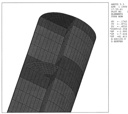
The acoustic test chamber is a 52 in. long, 11.75 in. diameter steel pipe with low frequency speakers at the top and bottom ends. The configuration for this research includes a 0.032 in. thick aluminum plate inserted 11 in. below the top speaker to divide the chamber into two sections. The chamber has circular symmetry about its vertical axis, and keeping this symmetry in the mesh of the finite element model will allow for an investigation of a reduced solution method called circulance (Appendix B). The mesh chosen for the divid-ing plate is a modification of that used by Grocott in his work on flexible active mirrors. [Grocott, 1997]

A MATLAB code is used to create geometric entities (keypoints and areas) for the mesh. This geometry is imported into ANSYS for meshing with quadrilateral and triangular shell elements with 6 degrees of freedom (DOF) per node (three translations and three rotations,

x). A clamped boundary condition is used around the edge of the plate. The two

dimen-sional plate mesh is then extruded vertically to form triangular and rectangular prism acoustic elements. These elements have only 1 DOF per node (pressure, P) except at the interface with a structure where they have 7 (6 structural and 1 pressure). A rigid bound-ary condition is assumed by ANSYS for the acoustic fluid except where it is in contact with a flexible structure. Finally, the speakers on the top and bottom of the chamber are modeled as relatively rigid shell elements with a grounded spring accounting for the single DOF piston motion of the speakers.

32 FINITE ELEMENT MODELING ANSYS 5.3 APR 1 1998 17:55:41 PLOT NO. 1 ELEMENTS TYPE NUM XV =-.1743 YV =-.8731 ZV =-.4552 *DIST=10.354 *XF =-1.995 *YF =-7.638 *ZF =41.413 A-ZS=136.9 Z-BUFFER

Figure 2.1 ANSYS mesh of chamber finite element model with wedge cutaway from acoustic

elements to expose structural components.

Since there is only 1 pressure DOF at each node, and the plate creates a pressure disconti-nuity between the top and bottom sections of the chamber, a second "dummy" set of shell elements must be created for the plate with nodes coincident with the first. This "dummy" plate is given no structural stiffness or mass, but the structural DOF are coupled to those of the actual plate model. This technique does not affect the structural behavior of the plate, but allows for separate pressure DOF on the upper and lower side of the plate which is required. This method is not necessary for the speaker models since they only interface with the acoustic elements on one side. The back-side acoustic stiffness of the speakers is lumped into the spring using measured data of the speakers outside the chamber.

The unforced finite element equations of motion in nodal coordinates are given in (2.1). [ANSYS Users Manual, 1992] In this equation, the subscripts spt, spb, p, ft, and fb

corre-Structural Acoustic Modeling in ANSYS 33

spond to the top speaker, bottom speaker, plate, top acoustic chamber, and bottom acoustic chamber respectively. These equations show how the fluid-structure coupling matrices Aspt , Aspb, Apt, and Apb enter the mass and stiffness matrix, and the unsymmetric nature of the coupled system.

Mspt 0 0 0 0 0 Mspb 0 0 0 0 0 Mp 0 0 + (2.1) -PAspt 0 -pApt Mft 0 0 -pAspb -pApb 0 Mfb Kspt 0 0 Aspt 0 0 Kspb 0 0 Aspb 0 0 K, Apt Apb

~I

The unsymmetric matrix equations of motion can be solved directly in ANSYS using an iterative solution method. This method is computationally expensive, and can be avoided if the uncoupled mode shapes form an acceptable basis for the coupled system. This is a valid assumption for this model since the plate and speakers are massive and stiff com-pared to the acoustic fluid. This assumption allows for the use of the Lanchoz method to efficiently solve for the mass normalized mode shapes and frequencies of the two speak-ers, plate, and two acoustic enclosures separately. Each of these uncoupled systems are symmetric, and can be solved directly. Additionally, a partial solution is run in ANSYS to create the full unsymmetric mass and stiffness matrices, and the fluid structure coupling matrices are extracted. The next section will explain how the component modes and cou-pling matrices are assembled to form a coupled modal state space model.

34 FINITE ELEMENT MODELING

2.3 Modal State Space Approach

The method to create a modal state space model using the uncoupled component modes and fluid structure coupling matrices is presented by Glaese. [Glaese, 1997] The first 40 modes of the plate, 26 modes of the upper acoustic chamber, and 30 modes of the lower acoustic chamber are used along with the piston modes of the two speakers. This set includes all of the component modes up to 1250 Hz.

Equation (2.2) shows the coordinate transformation from nodal coordinates to modal coor-dinates using the uncoupled component modes. This transformation is applied to (2.1), and the unforced system is pre-multiplied by T to give the modal equations of motion (2.3). Recall that the component modes were each mass normalized. This eliminates the need to perform all of the matrix multiplications except for the coupling terms, and the modal mass and stiffness matrices take the form given in (2.4)

A diagonal modal damping matrix is used as shown in (2.5). The damping ratios are a variable used to correlate the finite element model to data from the chamber. Table 2.1 lists the damping ratios used for the chamber configuration in this thesis. The damping ratio of the first structural mode is high because of its coupling to both acoustic chambers. The damping of the top acoustic chamber reflects thick acoustic foam used to simulate a far field effect. The damping of the bottom acoustic chamber reflects the use of a fiber-glass blanket to simulate acoustic blankets present in payload fairings.

TABLE 2.1 Modal damping ratios for finite element model

Mode Description Damping Ratio (r)

Speaker Piston Mode 0.102

First Symmetric Plate Mode 0.06

All Other Plate Modes 0.03

Top Chamber Acoustic Modes 0.2

Modal State Space Approach 35 spt 0 0 0 0 0 Ospb 0 0 0 0 0 ,O 0 0 0 0 0 ,ft 0 0 0 0 0 Ofb q= IDq Mspt 0 0 0 0 0 Mspb 0 0 0 0 0 Mp 0 0 -PAspt 0 -pAp, Mft 0 0 -pAspb -pApb 0 Mfb Kspt 0 0 Aspt 0 0 Kspb 0 0 Aspb 0 0 Kp Apt Apb Dq = 0 0 0 0 Kft 0 0 0 0 0 Kfb 0 0 00 I 0 00 0 I 00 P0-pTft Apt p I 0 -pTfb Aspb spb -P Tfb Apb p 0 I 2 0 0 Qspb 0 _{T Tspt Aspt} ft 2 0 0 0 _{0 n2} TpApt ft 0 0 0 Qft2 0 Tspb Aspb _fb T pApb Ofb 0 0 fb2

r

=

Lx

36 FINITE ELEMENT MODELING 2_{;spt Qspt 0 0 0 0} 0 2 _{spb spb 0 0 0} Cr = 0 0 2;pp 0 0 (2.5) 0 0 0 2;ft ft 0 0 0 0 0 2 ;fb Lfb

With the modal mass, stiffness and damping matrices known, the modal state space system matrix (A) can be assembled in the standard manner. This involves pre-multiplying (2.3) by Mr- 1, and solving for i. The state space system is shown in (2.6), with the form of the A matrix given explicitly. To complete the state space model, the effect of various sensors and actuators must be modeled and transformed to modal coordinates to form the forcing, sensing and feed-through matrices (B,C and D). Sensor and actuator modeling is the topic of the next section.

LI

-M 1Kr -M C r [B

Y = C + Du

2.4 Sensor and Actuator Modeling

Sensors and actuators are modeled to capture their effect on the input/output behavior of the chamber. The basic method for modeling the sensors and actuators involves 4 steps:

* Model the stiffness and mass of the sensor or actuator in ANSYS so the modal basis will reflect these passive properties.

* Create the forcing or sensing matrices in nodal coordinates. This may be as simple as selecting a single DOF, or involve interpolating between nodal positions and sum-ming the effect of a distributed sensor or actuator.

Sensor and Actuator Modeling 37

post-multiplying a sensing matrix by Q(.

0 Model any sensor or actuator dynamics that are within the bandwidth of the finite element model.

Figure 2.2 is a block diagram of the input/output model. Note that both the input and out-put variables are voltage which must be related to physical forces and sensed variables through sensor and actuator modeling.

Actuator u sq q C Sensor

Dynamics Dynamics

Figure 2.2 Block diagram of input/output characteristics of finite element model.

2.4.1 Microphones

Modeling a microphone is described first since it is the simplest of the sensors and actua-tors. The microphones are physically placed inside the acoustic chamber, and do not sig-nificantly affect the acoustics since the dimension of the microphones is much less than the smallest acoustic wavelength of interest. This eliminates the need for step one in the modeling process. Additionally, the sensing matrix in nodal coordinates simply selects the pressure DOF of the node where the microphone is placed. The model is not very sensi-tive to exact microphone location, so interpolation of pressure between nodes in not neces-sary. Finally, the microphone dynamics are well above the bandwidth of the model, and can be ignored without affecting the fidelity. This reduces the sensor dynamics to a scalar representing the gains in the data acquisition system.

38 FINITE ELEMENT MODELING

Equation (2.7) is a typical sensing matrix in nodal coordinates. The sub-matrices Cyx,

Cy, Cyi, and Cyp, select the nodal structural and pressure DOF and their derivatives

which form the output characteristics of the sensor. For a microphone, the only non-zero submatrix is Cyp. Equation (2.8) shows the transformation to modal coordinates, and explicitly how only part of this transformation is necessary due to the sparseness of Cy

C = C(2.7)

x

Cy ICyx Cyp Cy. Cy1 P

P

Cmic = kCy oq- = k 0 C t 0 0 I (2.8)

2.4.2 Accelerometers

An accelerometer is slightly more difficult to model than a microphone since acceleration is not a state variable. Accelerometers can be placed on any of the structural components in the chamber, and the mass of the accelerometer may significantly affect the dynamic response. For this research, Endevco 2222 accelerometers are used, and their passive effect is modeled in ANSYS as a concentrated mass (ig) at the node closest to the actual location. A complication of the accelerometer output matrices is that a feedthrough term exists (D) if the actuator and accelerometer are located on the same component structure. As was the case with the microphone, the accelerometer dynamics are well above the bandwidth of the model, and can be ignored.

Since the state space equations for the system are in modal coordinates, it is more straight-forward to derive the accelerometer output matrices in modal coordinates and then trans-form back to nodal coordinates. The left side of (2.6) includes an expression for

4

Sensor and Actuator Modeling 39

terms of the state variables and the applied modal force, u. Equation (2.9) shows the out-put equation for acceleration in modal coordinates.

= M Kr -MrCI C I +Bu (2.9)

The left side of this equation is transformed to nodal coordinates, but the right side is left in terms of modal state variables and forces. This results in a matrix equation with a row corresponding to the acceleration of each nodal DOF as shown in (2.10).

= D Mr1Kr -M-1 C[ + Bu= Cacc + Dacc U (2.10)

Only one row of this equation is needed for each accelerometer corresponding to the nodal DOF that the accelerometer senses. This results in a single row for Cacc and a scalar for

Dac_{c •}

Due to the coupling between the fluid and structure, Cacc includes terms multiplying the modal displacement and velocity states of the component structure, and the modal pres-sure states of any fluid interfacing with the structure (but not the prespres-sure velocity states). At first it is not intuitive why the acceleration of the structure should be a function of the acoustic modes, but this is physically explained by thinking of the pressure states as a dis-tributed force acting on the structure. Just as a force acting on the plate directly influences its acceleration though the Dacc matrix, forcing the acoustics (either directly or indirectly through a speaker model) will directly influence the acceleration of the plate through the coupling in the Cacc matrix even though Dace is zero for this pair of actuator and sensor.

2.4.3 Strain Gages

Like an accelerometer, a strain gage does not directly measure a state variable. Strain gages can be bonded to the aluminum plate at any location and direction to provide a mea-sure of the strain at that point on the plate. The addition of strain gages to the plate does

40 FINITE ELEMENT MODELING

not significantly affect the dynamics of the plate since the gages are light and by design very flexible. Modeling the output characteristics of a strain gage requires an interpolation of the nodal solution so the curvature of the plate can be approximated at any given point and direction.

The bending strain in an elastic material is given by (2.11). [Gere and Timoshenko, 1990] A cubic interpolation matching the nodal solution at the four closest nodes to the strain gage is necessary to evaluate the curvature. The interpolation function is derived from a general bi-cubic polynomial with 16 constants subject to the constraint that it satisfy the steady state Kirchoff plate theory equation (2.12). [Craig, 1981, Strang, 1986]

2

_ w(-hi

w(x, y) = c1 + c2x + c3x + c4x + c5Y + C6Y + C7Y + C8XY + c9xY (2.13)

3 2 3

+ cloxy + cllx y + cl2x y

The resulting bi-cubic interpolation (2.13) has 12 unknown constants which can be expressed as a combination of the state variables by matching the vertical displacement and two slopes at each of the four nodes. Since the state variables are in cylindrical coor-dinates, the substitutions x = rcos0, and y = rsin0 must be made which results in the appropriate cubic interpolation (2.14). Figure 2.3 is a sketch of the nodal locations used for the interpolation. The slopes are denoted as rotations about the r and 0 coordinates with Rr = , and Re - D. The curvature at a specific point is obtained by

differen-wO ' ar

tiating (2.14) twice with respect to the direction of measured strain. This is inserted into (2.11) to produce the strain output matrix in nodal coordinates Cy. A transformation simi-lar to (2.8) is used to transform this output matrix to modal coordinates.

Sensor and Actuator Modeling 41

(r4,04) (r3,03)

0

(r,O)

(r1,01) _(r2,02)

Figure 2.3 Sketch of nodal locations and coordinate directions for bi-cubic interpola-tion of FEM results.

w(r, 0) = c1 + c2rcosO + c3r2(cosO)2 + c4r3(cosO)3 + c5rsinO (2.14)

+ c6r2(sin0)2 + c7r3(sinO)3 + c8r2 osOsinO + cr3 COSO(sinO)2

4 3 3 2 4 3

+clor cosO(sinO) +cll r sinO(cosO)2 + c12r sinO(cos0)3

2.4.4 Speakers

The speakers at the top and bottom of the test chamber are essentially pressure actuators which are used to excite the acoustics in the chamber. The simplest model of the speakers would be to directly drive the pressure DOF's at the speaker location. This approach may be valid for very low frequency excitation; however, the speakers have both mechanical and electrical dynamics within the bandwidth of the model. These dynamics must be cap-tured if the fidelity of the model is to be maintained.

The coupled electro-mechanical model of the speaker is given by (2.15), where the con-stants are defined in Table 2.2. [Glaese, 1997] The expanded form of (2.15) shows that with an approximation to the mechanical damping, the system can be decoupled into a mechanical model and a disturbance model. This approximation is reasonable since damping is added to the model as a correlation variable to match the input/output

charac-42 FINITE ELEMENT MODELING

teristics, and not a strictly modeled physical parameter. As described in Section 2.2, the speaker is modeled in ANSYS as a single DOF oscillator, and with the addition of modal damping, the entire mechanical model of the speaker is captured in the modal state space formulation. 0 1 0 k c BI m _{m mL} e Re 0 B -Le x+ 0 +L )+kx + 0 - mX + + kx= V sLe + Re sLe + Re iV V x

TABLE 2.2 Physical parameters of speaker

The right side of (2.15) forms the speaker disturbance model which describes how a drive voltage, V, results in a modal force actuation of the speaker. This is inserted into the "Actuator Dynamics" block of Figure 2.2, and augmented to the mechanical dynamics when calculating the input/output response due to excitation of the speaker. The remain-ing part of the speaker model involves determinremain-ing the input matrix (B) for the speaker. This follows a similar formulation to that of C for the sensors.

Since only one mechanical mode of each speaker is retained in the modal state space model, the forcing vector for the speaker in nodal coordinates is somewhat arbitrary as long as it results in excitation of this mode. A single force acting at the center node of the speaker in the positive z-direction for the bottom speaker and negative z-direction for the top speaker is used. This results in a single non-zero entry in the nodal forcing vector for

i

Electrical Resistance (Re) 11.9 2 Electrical Inductance (Le) 2.25 x 10-3 H Electro-mechanical Coupling (Bl) 9.83 N/A

Sensor and Actuator Modeling 43

each speaker. This forcing vector is transformed to modal coordinates as shown in (2.16) The scalar k represents the gain of the amplifier used to drive the speaker.

O 0 T Bs = kMrT 1 = kM-1 sp 1 (2.16) sp r r 0 0 0 0

2.4.5

Piezoelectric Sensors and Actuators

Piezoelectric materials bonded to a structure are commonly used as both actuators and sensors for structural and acoustic control. These actuators and sensors are naturally dis-tributed, and can be placed on the structure or shaped to provide favorable modal observ-ability and controllobserv-ability. For this research, PZT wafers are used as structural actuators and/or sensors, and PVDF film is used as a modally shaped sensor. The modeling of both relies on the ability to characterize the electro-mechanical behavior of the material in terms of forces or displacements around its contour.

PZT Actuator

A 2.5" x 1.5" x 0.01" PZT wafer bonded to the aluminum plate is used as the structural

control actuator. The wafer adds considerable mass and stiffness to the plate, and is mod-eled in ANSYS by altering the density and modulus of the shell elements in the vicinity of the wafer. The added stiffness contribution is calculated using laminated plate theory con-sidering the plate and wafer as separate laminates. Since the wafer is rectangular and the finite element mesh is circular, the added mass and stiffness is approximated over a 1.5" diameter circle at the center of the plate.

A method developed by Griffin and Henderson was used which treats the actuation of the PZT as the blocked force acting against the finite element model of the plate and wafer. This force results in a distributed moment around the edge of the wafer, as shown in Figure 2.4, due to the offset of the wafer from the neutral axis of the plate. The modeling

44 FINITE ELEMENT MODELING

method has been validated with experimental data for aluminum plates 0.018in to 0.125in thick. [Griffin & Henderson, 1997]

Y

7-4

MxMy

a

Figure 2.4 Edge moment actuation of PZT wafer.

The equations of motion for the plate with PZT actuator are given in (2.17). The left side of this equation comes from Kirchoff plate theory, and is captured by the finite element model. The terms on the right side are distributed forces applied by the piezoelectric material and reduce to distributed moments along the edge of the PZT when integrated over the area using the finite element shape functions. These distributed moments are given in (2.18) with the variables described in Table 2.3.

2 2 Eh 4w + Mx(pe) My(pe) (2.17) 3(1 - ) y2 Ox2 Epe a(tpe_+ h) (2.18) Mx p (2.18) pe M y 1 - upe _n 2

Sensor and Actuator Modeling 45

TABLE 2.3 Constants used for modeling PZT wafer on aluminum plate

Piezoelectric Modeling Variable Value Piezo Elastic Modulus (Epe) 8.833x106 psi

Piezo Poisson's Ratio (upe) 0.35

Transverse Piezo Strain Constant (d31) 6.7333x10-9 in/V

Piezo Thickness (tpe) 0.01 in.

Plate Thickness (h) 0.032 in.

Edge Length of Distributed Moment (a,b) a = 2.5 in. b = 1.5 in. Discretization Points Along Edge (n) 10

The cubic interpolation function developed in Section 2.4.3 is used to apply this distrib-uted moment at 10 discrete points along each edge of the wafer. Since the finite element model is in cylindrical coordinates, and the applied moments are described in Cartesian coordinates, an additional coordinate transformation (2.19) is necessary. This produces a forcing vector in nodal coordinates that is a function of the displacement states of several nodes near the edge of the wafer. The transformation to modal coordinates and addition of the scalar gain for the amplifier completes the input model for the PZT actuator.

S cos0 -- sinO

a x _ r ₁ 8

a

aw sin0 !cosj

aw

PVDF Sensor

Two circularly shaped PVDF sensors are used to provide high modal observability of the first and second symmetric plate modes while filtering the response of the asymmetric modes. PVDF film is extremely thin, and does not affect the dynamics of the plate. An analog charge amplifier circuit is used to produce an output voltage proportional to the charge on the PVDF electrode, which is in turn proportional to the area integral of strain.

46 FINITE ELEMENT MODELING

The signal voltage of PVDF bonded to a plate is the area integral of the strain multiplied by the transverse piezoelectric strain constant (2.20). It is seen that for a circular sensor,

aw

the contribution of the second integral is zero, and the signal reduces to the integral of

r

around the contour of the sensor. This integral is approximated as a summation of 100 dis-crete points along the contour, and the interpolation function of Section 2.4.3 is used to relate this summation to the state displacement variables of the nodes near the contour. This results in a sensor matrix in nodal coordinates that is transformed to modal coordi-nates in the same manner as (2.8).

2nR 2 R2r 2

y = d31 f w(r, 0)ara0 + d31 w(r, )a8ar (2.20)

0 oa r 220 0 ao

27t R

t 8 ta _ w

d312 fJ w(R, O)aO + d312 w(r, 2) - aw(r, 0)ar

0 0

n

t a 2nrR

d312 rw(R,i) )n

i= 1

The same modeling approach is used for a PZT wafer acting as a distributed sensor. For this case, the integral in (2.20) is carried out in Cartesian coordinates over the area of the wafer, and reduces to a summation of line integrals over each edge. Again, the interpola-tion funcinterpola-tion is used to discretize this integral, and the two coordinate transformainterpola-tions are applied to transform to cylindrical and modal coordinates.

2.5

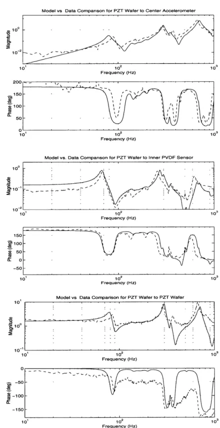
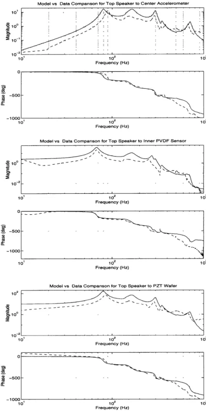
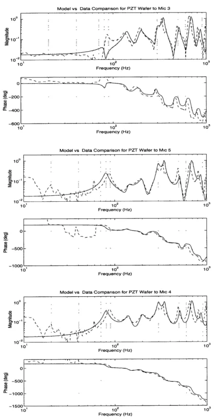
Open-Loop Model Correlation

Open-loop correlation of the finite element model is accomplished by comparing transfer functions from the control and disturbance actuators to the feedback and performance sen-sors. With few exceptions, this comparison shows that the finite element model captures the coupled dynamics of the chamber. Table 2.4 summarizes this correlation by compar-ing the frequency of the uncoupled and coupled component modes. This shows that the model captures the significant stiffening of the first plate mode and two speaker modes, as well as the de-stiffening of the first lower chamber acoustic mode.