HAL Id: hal-01671603
https://hal.sorbonne-universite.fr/hal-01671603
Submitted on 22 Dec 2017HAL is a multi-disciplinary open access archive for the deposit and dissemination of sci-entific research documents, whether they are pub-lished or not. The documents may come from teaching and research institutions in France or abroad, or from public or private research centers.
L’archive ouverte pluridisciplinaire HAL, est destinée au dépôt et à la diffusion de documents scientifiques de niveau recherche, publiés ou non, émanant des établissements d’enseignement et de recherche français ou étrangers, des laboratoires publics ou privés.
Seasonal radiative modeling of Titan’s stratospheric
temperatures at low latitudes
Bruno Bézard, Sandrine Vinatier, Richard K. Achterberg
To cite this version:
Bruno Bézard, Sandrine Vinatier, Richard K. Achterberg. Seasonal radiative modeling of Ti-tan’s stratospheric temperatures at low latitudes. Icarus, Elsevier, 2018, 302, pp.437 - 450. �10.1016/j.icarus.2017.11.034�. �hal-01671603�
Seasonal radiative modeling of Titan’s stratospheric temperatures
at low latitudes
Bruno Bézard
a*, Sandrine Vinatier
a, Richard K. Achterberg
ba
: LESIA, Observatoire de Paris, PSL Research University, CNRS, Sorbonne
Universités, UPMC Univ. Paris 6, Université Paris-Diderot, Sorbonne Paris
Cité, 5 place Jules Janssen, 92195 Meudon, France
b
: University of Maryland, Department of Astronomy, College Park, MD 20742,
United States
*
Corresponding author.
E-mail address: bruno.bezard@obspm.fr
Contact details: Bruno Bézard LESIA, Bât. 18
Observatoire de Paris, section de Meudon 92195 Meudon cedex
France
Phone: (33) 1 45 07 77 17 Fax: (33) 1 45 07 28 06
Published in Icarus, Volume 302, 1 March 2018, Pages 437–450 https://doi.org/10.1016/j.icarus.2017.11.034
ABSTRACT
1 2
We have developed a seasonal radiative-dynamical model of Titan’s stratosphere to 3
investigate the temporal variation of temperatures in the 0.2-4 mbar range observed by the 4
Cassini/CIRS spectrometer. The model incorporates gas and aerosol vertical profiles derived 5
from Cassini/CIRS and Huygens/DISR data to calculate the radiative heating and cooling rate 6
profiles as a function of time and latitude. At 20°S in 2007, the heating rate is larger than the 7
cooling rate at all altitudes, and more specifically by 20-35% in the 0.1-5 mbar range. A new 8
calculation of the radiative relaxation time as a function of pressure level is presented, leading 9
to time constants significantly lower than previous estimates. At 6°N around spring equinox, 10
the radiative equilibrium profile is warmer than the observed one at all levels. Adding 11
adiabatic cooling in the energy equation, with a vertical upward velocity profile 12
approximately constant in pressure coordinates below the 0.02-mbar level (corresponding to 13
0.03-0.05 cm s-1 at 1 mbar), allows us to reproduce the observed profile quite well. The 14
velocity profile above the ~0.5-mbar level is however affected by uncertainties in the haze 15
density profile. The model shows that the change in insolation due to Saturn’s orbital 16
eccentricity is large enough to explain the observed 4-K decrease in equatorial temperatures 17
around 1 mbar between 2009 and 2016. At 30°N and S, the radiative model predicts seasonal 18
variations of temperature much larger than observed. A seasonal modulation of adiabatic 19
cooling/heating is needed to reproduce the temperature variations observed from 2005 to 2016 20
between 0.2 and 4 mbar. At 1 mbar, the derived vertical velocities vary in the range -0.05 21
(winter solstice) to 0.16 (summer solstice) cm s-1 at 30°S, -0.01 (winter solstice) to 0.14 22
(summer solstice) cm s-1 at 30°N, and 0.03-0.07 cm s-1 at the equator.
23 24
Key words: Titan, atmosphere; Atmospheres, structure; Atmospheres, dynamics 25
1. Introduction
27
Due to Saturn’s obliquity of 26.7°, Titan experiences large seasonal variations of insolation. 28
The 0.056 eccentricity of Saturn’s orbit adds a significant modulation to this insolation. 29
Above the 10-mbar level, Titan’s radiative time constant is less than a Titan year (29.5 Earth 30
years) (Strobel et al. 2009, Flasar et al. 2014) so that significant seasonal variations of 31
temperature are expected in the mid-stratosphere and mesosphere. 32
33
Infrared observations by the IRIS instrument aboard the Voyager 1 spacecraft in November 34
1980 pointed out a north-to-south asymmetry of temperatures in the 0.4-1 mbar region, with 35
temperatures at 55°S being higher than at 55°N by 4 and 8 K at 1 and 0.4 mbar respectively 36
(Flasar et al. 1990). These observations occurred shortly after northern spring equinox, at a 37
heliocentric longitude Ls ≈ 9°. Flasar and Conrath (1990) proposed that the asymmetry was
38
due to a phase lag in the response of the atmosphere to the seasonally-varying insolation due 39
to dynamical inertia. On the other hand, Bézard et al. (1995) suggested that the asymmetry 40
results from the larger concentrations of infrared radiators (photochemical gases and aerosols) 41
present at high northern latitudes. 42
43
The Cassini Composite Infrared Spectrometer (CIRS) aboard Cassini allowed us to monitor 44
the thermal structure of Titan’s stratosphere from July 2004 to September 2017, which 45
corresponds to Ls ≈ 293°. Combining limb- and nadir-viewing observations between 2004 and
46
2006, Achterberg et al. (2008a) retrieved the temperature field over the pressure range 5×10⁻³ -47
5 mbar from about 75°S to 75°N. The corresponding season was around northern mid-winter 48
(Ls = 293-323°). Compared with Voyager 1 observations, the north-to-south asymmetry was
49
stronger and temperatures at 55°S were higher than at 55°N by about 18 and 11 K at 1 and 0.4 50
mbar respectively. Compared to southern latitudes, high northern latitudes were then 51
experiencing reduced solar heating and enhanced abundances of photochemical gases and 52
aerosols, both of which likely contribute to the lower temperatures. Besides this asymmetry, 53
mid-stratosphere temperatures on Titan were reaching their maximum at latitudes 0-30°S. On 54
the other hand, the stratopause was found higher and warmer beyond 50°N than anywhere 55
else on the satellite, which very likely results from adiabatic heating from downwelling air at 56
winter polar latitudes. Achterberg et al. (2011) extended the analysis of Achterberg et al. 57
(2008a) using Cassini/CIRS data up to December 2009, i.e. shortly after northern spring 58
equinox (Ls ≈ 4°). Between 2004 and 2009, a large decrease of temperatures in the stratopause
59
region (above the 0.1-mbar level) was found beyond 30°N. Elsewhere in the stratosphere and 60
lower mesosphere, the temperature variations did not exceed 5 K. 61
62
The temporal and latitudinal variations of temperature observed in the stratosphere and lower 63
mesosphere result from combined variations of the insolation, modulating the solar heating 64
rate, of the atmospheric composition, which governs the radiative cooling and solar heating 65
rates, and of dynamical motions, which provide adiabatic heating and cooling. To try to assess 66
the relative importance of these actors, it is first necessary to constrain as precisely as possible 67
the radiative forcing terms, which requires a good knowledge of the distribution of the 68
radiatively-active gases and aerosols. Such information is available from Cassini/CIRS, which 69
measures in nadir- and limb-viewing geometry the thermal emission spectrum of Titan from 70
10 to 1495 cm-1. This allows the retrieval of the gas concentration and aerosol extinction 71
profiles that contribute to the radiative cooling between approximately 130 and 450 km (5-72
0.005 mbar) (e.g. Vinatier et al. 2010a, 2010b, 2015). The Descent Imager/Spectral 73
Radiometer (DISR) aboard the Huygens probe measured the optical properties and vertical 74
distribution of haze particles between 0 and ≈150 km (Tomasko et al. 2008c, Doose et al. 75
2016) on 14 January 2005 near 10°S. Used with a correct representation of the methane 76
opacity, these results allow us to compute the solar heating rate profile as a function of zenith 77
angle. Combining Huygens/DISR and Cassini/CIRS data, Tomasko et al. (2008b) were able 78
to investigate the heat balance at the location and time of the Huygens descent. They inferred 79
that the day-averaged solar heating rate profile exceeded the cooling rate profile by a 80
maximum of 0.5 K/Titan day (0.03 K/Earth day) near 120 km altitude (5.5 mbar) and 81
concluded that the general circulation must redistribute this heat to higher latitudes. 82
83
In Titan’s stratosphere, a meridional circulation, similar to Hadley cells on Earth, is driven by 84
the latitude-dependent solar heating (see a review of Titan’s general circulation in Lebonnois 85
et al. 2014). General Circulation Models (GCMs) have been developed to investigate Titan’s 86
dynamics, in particular the superrotation characterized by prograde zonal winds up to ~200 m 87
s-1 in the winter stratosphere (see Newman et al. 2011, Lebonnois et al. 2012 and Lora et al. 88
2015 for recent three-dimensional GCMs). These models show a pole-to-pole circulation, 89
particularly in the stratosphere, with rising motion in the summer hemisphere and subsidence 90
in the winter hemisphere except around equinox, when a more symmetric equator-to-pole 91
circulation takes place throughout the atmosphere. They generally succeed in reproducing at 92
least qualitatively the dominant features of Titan’s atmospheric structure, such as the zonal 93
wind pattern and temperature field, but suffer from approximations in the treatment of the 94
radiative transfer and/or various other simplifications. The strong subsidence at high winter 95
latitudes predicted by the GCMs is confirmed by the high temperatures and the large 96
enrichment in minor photochemical species observed in the upper stratosphere and 97
mesosphere (Achterberg et al. 2011; Teanby et al. 2007, 2009; Vinatier et al. 2007, 2010a). 98
The temperature anomalies observed in winter around the north pole have been used to 99
estimate downward vertical velocities of ~10 cm s-1 around 0.01 mbar in 2005-2007
100
(Achterberg et al. 2011). Changes in the vertical abundance profiles of minor species 101
observed near the south pole in autumn were also used to derive the following vertical 102
velocities: from 0.1 to 0.4 cm s-1 near 0.003 mbar in 2010-2011 and 2011-2012 (Teanby et al. 103
2012, Vinatier et al. 2015), 0.25 cm s-1 near 0.01 mbar in 2011-2012, and 0.4 cm s-1 near 0.02
104
mbar in 2015 (Vinatier et al. 2017a). 105
106
The goal of this paper is to investigate the heat balance of Titan’s stratosphere using a 107
seasonal radiative model based on measurements by Cassini/CIRS of the distributions of the 108
radiative agents and state-of-the-art representation of gas and aerosol spectral properties. We 109
also take into account constraints from Huygens/DISR measurements. We then calculate the 110
season-dependent radiative solution for the temperature profile and compare it with the 111
observed variations of temperature at different levels and latitudes to derive constraints on the 112
dynamical heating/cooling. Here, we restrain our analysis to mid-latitudes (30°S-30°N) where 113
gas and aerosol do not exhibit large seasonal variations. Section 2 describes the temperature 114
data, retrieved from Cassini/CIRS measurements, with which we are comparing our model. 115
Section 3 presents our seasonal radiative model and the gas and aerosol distributions used in 116
the radiative transfer code to calculate heating and cooling rates. Radiative model results are 117
presented in Section 4 and compared with observations to constrain the missing adiabatic 118
heating and cooling terms. Also shown is a calculation of the radiative time constant as a 119
function of pressure level. We discuss these results in Section 5 and present our conclusions 120 in Section 6. 121 122 2. Observations 123
Retrievals of Titan’s temperature field are routinely achieved using nadir and limb 124
observations of the ν4 band of methane through Focal Plane FP4 of Cassini/CIRS. This focal
125
plane covers the interval 1050-1495 cm-1 at a spectral resolution adjustable from 15.5 to 0.5 126
cm-1 (apodized). It consists of a 10-pixel linear array, with a 0.27-mrad field of view (FOV) 127
per pixel (Flasar et al. 2004). Temperature maps were retrieved by Achterberg et al. (2008a) 128
for mid-winter conditions (2004-2006) combining nadir-viewing (2.8-cm-1 resolution) and
129
limb-viewing (15.5-cm-1 resolution) sequences. The nadir data cover latitudes from 90°S to 130
60°N and yield information in a pressure range of about 5-0.2 mbar while the limb data cover 131
latitudes from 75°S to 85°N and yield information in a pressure range ≈ 1-0.005 mbar. 132
Achterberg et al. (2011) extended the analysis to cover 5.5 years of Cassini/CIRS 133
observations from July 2004 to December 2009, just after northern spring equinox. Here we 134
use a further extended data set encompassing observations up to June 2016, i.e. Titan flybys 135
T0 to T118 (Achterberg et al. in preparation). For each flyby, zonal-mean temperatures were 136
obtained by zonally averaging temperatures retrieved from individual nadir-viewing spectra 137
(2.8-cm-1 resolution) using 5° latitude bins with 2.5° spacing and interpolating the retrieved 138
temperatures onto a uniform latitude grid for each flyby. Averaging was done in a reference 139
frame that removes the 4° offset of the stratospheric symmetry axis from the surface pole 140
(Achterberg et al. 2008b). In our analysis, we used temperatures retrieved at 0.2, 0.5, 1, 2 and 141
4 mbar, which cover the range of maximum temperature information. Note that these 142
temperatures actually represent a vertical average over 1 to 1.5 scale heights due to the width 143
of the contribution functions in the methane band and the filtering applied in the retrieval 144
process. We restrained our analysis to equatorial and mid-latitudes and selected data at q = 0°, 145
30°N and 30°S. For a given latitude q and a given flyby, we averaged the three temperatures 146
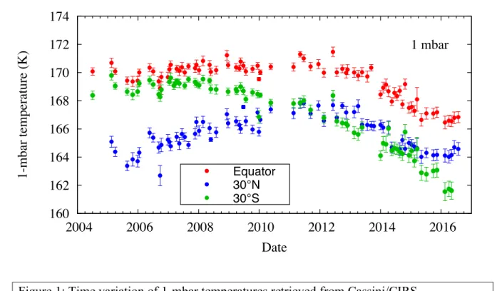
retrieved by Achterberg et al. (in preparation) at latitudes q-2.5°, q and q+2.5°. Figure 1 147
shows the retrieved 1-mbar temperatures as a function of time for these three latitudes. The 148
error bars correspond to the standard deviation (SD) of temperatures in each 5° bin divided by 149
square of root of the number of data points. Seasonal variations are clearly visible in this data 150
set. At the equator, the 1-mbar (~185 km) temperature increases slightly from 2005 to 2011-151
2012 (by less than 1 K), and decreases more noticeably after 2012 (by ~4 K between 2012 152
and 2016). At 30°N, the temperature increases by ~4 K from 2005 to 2012 and decreases by 153
about the same amount from 2012 to 2016, while at 30°S the temperature regularly decreases 154
by ~8 K from 2005 to 2016. 155
156
157
Vinatier et al. (2015) produced maps of temperature and composition from selected sequences 158
of CIRS limb spectra recorded between October 2006 and May 2013 at a resolution of either 159
0.5 or 15.5 cm-1. Reliable information extends from 5 to 0.001 mbar, a region below which 160
the temperature profile smoothly joins the Huygens/HASI profile measured in situ at 10°S in 161
January 2005 (Fulchignoni et al. 2005). We used Vinatier et al.’s results around 6°N, a 162
latitude least sensitive to seasonal effects, as a reference profile to test our model and 163
investigate the heat balance at this latitude. To smooth out small local temperature variations, 164
we averaged four temperature profiles recorded at 4-5°N, on January 2007 (Ls = 327°), 165
December 2009 (Ls = 4°), June 2010 (Ls = 11°) and May 2011 (Ls = 21°), thus corresponding 166
to northern mid-winter to mid-spring conditions. This profile is shown in Fig. 7. The 1-SD 167 160 162 164 166 168 170 172 174 2004 2006 2008 2010 2012 2014 2016 1-mbar temperature (K) Date 1 mbar Equator 30°N 30°S
Figure 1: Time variation of 1-mbar temperatures retrieved from Cassini/CIRS measurements at three latitudes, 0°, 30°N and 30°S.
formal error bar due to noise propagation is about ± 0.2 K in the range 0.1-1 mbar increasing 168
to ± 0.3 K at 0.01 mbar and ±0.4 K at 5 mbar. The standard deviation of our set of four 169
temperature profiles is larger, 0.5 to 1.5 K from 0.2 to 2 mbar, 2 K at 0.1 and 5 mbar and 5 K 170
at 0.01 mbar. 171
172
3. Seasonal radiative model
173
We developed a one-dimensional seasonal radiative-dynamical model to investigate the 174
observed temperature variations in Titan’s stratosphere. We solve for the energy equation: 175 !"($) !& = ℎ 𝑧 − 𝑐 𝑧 − 𝑤(𝑧) -($) ./ + !"($) !$ . (1) 176
h(z) is the solar heating rate equal to −.
-/
12∗ 4
14 , where F* is the downward solar flux, c(z) is
177
the radiative cooling rate equal to −.
-/
1256 4
14 with FIR being the upward thermal emission
178
flux, w the upward vertical velocity, Cp the specific heat, and g the acceleration of gravity. 179
The term 𝑤 𝑧 - $.
/ represents the adiabatic cooling rate and 𝑤 𝑧
!" $
!$ the cooling rate due to
180
vertical advection. The solar flux is calculated for diurnally averaged (i.e. zonally-averaged) 181
insolation. We neglect the meridional advection of heat. As discussed by Achterberg et al. 182
(2011) and Teanby et al. (2017), this term is expected to be ≤0.2 time the vertical advection 183
term, based on the mass continuity equation and the observed horizontal temperature 184
gradients, all the more at low latitudes where these temperature gradients are very small. 185
186
3.1 Solar flux 187
Our atmospheric grid consists of 41 pressure levels uniformly distributed in log-scale from 188
1.466 bar (surface pressure) to 0.133 µbar (around 650 km). The solar flux is calculated as a 189
function of zenith angle qs and altitude from 2610 to 40000 cm-1 (3.8-0.25 µm) using a plane 190
parallel radiative transfer code that incorporates the DISORT algorithm (Stamnes et al. 1988) 191
with 8 streams to solve for scattering. The solar irradiance spectrum at 1 AU is the 2000 192
ASTM Standard Extraterrestrial Spectrum Reference E-490-00 (available at 193
http://rredc.nrel.gov/solar/spectra/am0/). We consider opacity from methane and aerosols. 194
Methane absorption is modeled from 2610 cm-1 (3.8 µm) to 25000 cm-1 (0.400 µm) using the 195
correlated-k distribution method. From 2690 to 11850 cm-1, absorption coefficients are 196
calculated with a line-by-line radiative transfer model and molecular line parameters 197
(positions, intensities, energy levels) from the TheoReTS database, which includes new 198
accurate theoretical linelists of 12CH
4, 13CH4 and 12CH3D (Rey et al. 2017). The assumed N2
-199
broadened halfwidths and far wing lineshape are described in Rey et al. The CH3D/CH4 ratio
200
corresponds to D/H = 1.32´10-4 (Bézard et al. 2007). For each 40-cm-1 interval, a set of 16
k-201
coefficients, 8 for the interval [0:0.95] of the normalized frequency g and 8 for the interval 202
[0.95:1.00], is calculated on a set of pressures and temperatures. Beyond 11850 cm-1, we used 203
the coefficients of the Voigt-Goody band model calculated by Karkoschka and Tomasko 204
(2010, Table 4) based on methane transmission measurements from laboratory, Huygens and 205
HST data. We then essentially proceeded as in Irwin et al. (1996) and generated, for each 206
pressure and temperature of our set, 24 transmission (Tr) spectra with column densities (a) 207
equally spaced in log space between a minimum value such as Tr ≈ 0.997 and a maximum 208
value such as Tr ≤ 0.01. This function Tr(a) was then fitted with an exponential sum 209
characterized by 10-point Gaussian Legendre quadrature abscissae and weights, using a 210
Levenberg-Marquardt non-linear least squares algorithm (Press et al. 1997). The first guess of 211
the 10 ki absorption coefficients was derived from the k distribution of a Malkmus-Lorentz 212
band model (Eq. 12 of Irwin et al. 1996) having the S and B parameters given in Table 4 of 213
Karkoschka and Tomasko (2010). The function Tr(a) was actually fitted with the 10 214
parameters k1 and (ki-ki-1), for i = 2,10, discarding the iterations leading to negative values of 215
any of them, to ensure that they increase monotonically. We kept the original sampling of 216
Karkoschka and Tomasko (2010): 5 cm-1 in the interval 11850-19300 cm-1 and 25 cm-1 in the 217
interval 19300-25000 cm-1. 218
219
The methane mole fraction profile used in the radiative transfer is that derived by Niemann et 220
al. (2010) from the analysis of Huygens/GCMS in situ measurements, with a uniform mole 221
fraction of 1.48 ´ 10-2 above 45 km. The temperature profile T
0(p) is that retrieved by Vinatier
222
et al. (2010a) from Cassini/CIRS limb and nadir spectra recorded near 20°S in March 2007, 223
not far from the Huygens descent latitude. 224
225
The properties of the aerosol particles (single scattering albedo, phase function) were taken 226
from the recent reanalysis of Huygens/DISR observations by Doose et al. (2016, Table 2) 227
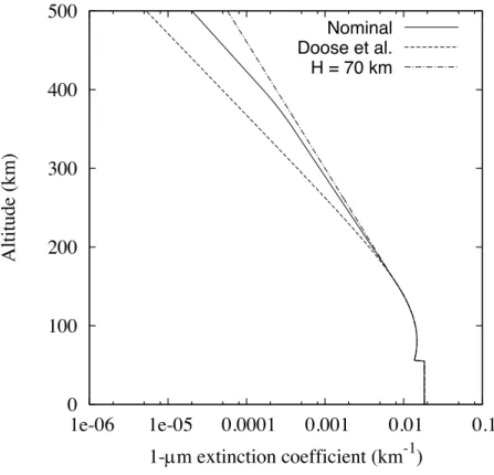
Figure 2: Haze extinction coefficient at 1 µm for our nominal model (solid line), Doose et al.’s (2016) model (dashed line) and one with a constant scale height of 70 km above 160 km (dash-dot line). In the thermal infrared range, at 1090 cm-1, these extinction profiles are scaled by factors of 0.0103, 0.0113 and 0.0099 respectively.
0 100 200 300 400 500 1e-06 1e-05 0.0001 0.001 0.01 0.1 Altitude (km) 1-µm extinction coefficient (km-1) Nominal Doose et al. H = 70 km
with information on the phase function from Tomasko et al. (2008c). Longward of 950 nm, 228
we used the single scattering albedo derived by Hirtzig et al. (2013) from modeling of 229
Cassini/VIMS data. We used the wavelength dependence of the extinction given in Table 2 of 230
Doose et al. (2016). The vertical variation of the extinction at the Huygens site is constrained 231
in detail between 0 and 144 km from the DISR measurements but only in average above this 232
altitude. Doose et al. then added the additional constraint of the optical limb altitude as 233
observed by Karkoschka and Lorenz (1997) to produce an analytical vertical profile of 234
extinction characterized, in the stratosphere, by an optical depth scale height decreasing from 235
large values below 80 km to a value of 65 km at 120 km and an asymptotic value of 45 km at 236
very high altitudes (Fig. 2). Here we considered additional constraints from Cassini/CIRS 237
measurements of the aerosol continuum emission in limb-viewing and nadir geometry 238
between 600 and 1500 cm-1. These measurements provide a vertical profile of the extinction 239
at thermal wavelengths with a good precision between approximately 140 and 400 km (3-0.01 240
mbar) (Vinatier et al. 2010b, 2015). We used here the vertical dependence of the extinction 241
determined from limb observations in January 2007 around 5°N (Vinatier et al. 2010a, b) and 242
adapted by Vinatier et al. (2015) (dashed line in their Fig. 15). Their extinction profile has a 243
scale height (H) of about ~65 km up to 350 km decreasing to ~48 km above 400 km. Our 244
nominal profile for the haze extinction is then the Doose et al. profile up to 160 km, that we 245
extend above with H = 65 km from 160 to 350 km, linearly decreasing to 48 km at 400 km 246
(Fig. 2). The extinction profiles derived from CIRS measurements at equatorial and mid-247
latitudes show however a significant variability with latitude and year above 250 km (Vinatier 248
et al. 2015, 2016). Although part of it may be an artifact due to uncertainties in the continuum 249
calibration, especially at high altitudes (≥ 400 km), most of it is probably real, including the 250
presence of the variable detached haze layer, as discussed in Vinatier et al. (2015). An 251
average of the profiles observed in 2010-2012 between 20°N and 30°S (Fig. 15 of Vinatier et 252
al. 2015) shows a vertical variation close to the Doose et al. profile up to 300 km and 253
intermediate between our nominal profile and Doose et al. up to 400 km. On the other hand, 254
observations at 26°S in January 2016 exhibit an approximately constant scale height H as 255
large as 70 km between 200 and 500 km (Vinatier et al. 2016). We consider that the full 256
Doose et al. profile and one having H = 70 km above 160 km represent a reasonable envelope 257
of the actual extinction profiles at low latitudes (Fig. 2). 258
259
We assumed a Lambertian surface with the reflectivity inferred by Jacquemart et al. (2008) 260
between 900 and 1600 nm from DISR/DLIS spectra taken at an altitude of 25 m and after 261
landing of the Huygens probe. The surface reflectivity down to 400 nm was obtained from 262
Eq. 5 of Karkoschka et al. (2012), giving the relative spectral variation of I/F derived from 263
DISR/DLVS data after landing, and scaled with the Jacquemart et al. value at 900 nm. 264
Between 250 and 400 nm, we assumed a linear variation of 4´10-4 nm-1 and, beyond 1600
265
nm, we used the Hirtzig et al. (2013) albedos derived from the methane windows in 266
Cassini/VIMS spectra near the Huygens landing site. We account neither for the strong 267
opposition effect seen in the phase function of Titan’s surface (Karkoschka et al. 2012) nor 268
for the fact that the surface at Huygens’ landing site is darker than average at low latitudes. 269
However, the influence of the surface reflectivity on the heating rate at stratospheric levels 270
should be relatively low. 271
272
3.2 Thermal emission 273
Without scattering, the thermal flux at pressure level p is equal to: 274 𝐹89 𝑝 = 2𝜋 𝑑𝜎 𝐵@ 𝑇 𝜏@C 𝐸 E 𝜏@C − 𝜏@ 𝑑𝜏@C − F GH 𝐵@ 𝑇 𝜏@ C 𝐸 E 𝜏@ − 𝜏@C 𝑑𝜏@C GH I F I , (2) 275
where ts is the optical depth at wavenumber s and pressure level p, Bs(ts’) is the Planck
276
function at the temperature T of the level of optical depth ts’ and wavenumber s, and E2 is
the second-order exponential integral (𝐸E 𝑥 = KLMN
&O 𝑑𝑡
F
Q ). The two terms in Eq. 2 represent
278
the fluxes from respectively the upwelling and downwelling radiation at pressure level p. We 279
calculate this integral from 20 to 1560 cm-1, and divide it into nk = 74 intervals of width ds = 280
20 cm-1. Thermal emission from outside this spectral interval can be neglected in the energy 281
budget. Our grid has np = 51 pressure levels uniformly distributed in log-scale from 𝑝Q
282
= 1.466 bar (surface pressure) to 𝑝R/ = 0.1466 µbar (around 650 km). By linearizing the 283
Planck function as a function of optical depth within each atmospheric layer of our grid [j, 284
j+1], and assuming that the Planck function is constant over each spectral interval k of width 285 ds, i.e.: 286 𝐵@S 𝑇 𝜏@C = 𝐵 @S 𝑇 𝑝T GH 4UVW XGHY GH 4UVW XGH 4U + 𝐵@S 𝑇 𝑝TZQ GHYXGH 4U GH 4UVW XGH 4U , (3) 287
Eq. 2 at a given pressure level pi can be written out as summations over indices k and j as: 288 𝐹89 𝑝[ = 𝜋 𝛿𝜎 ^HS " 4W _@ 2𝐸E 𝜏@ 𝑝Q − 𝜏@ 𝑝[ 𝑑𝜎 @SZ_@ E @SX_@ E + RS `aQ 289 Q _@ 𝑑𝜎 @SZ_@ E @SX_@ E 𝐵@S GH 4U GH 4UVW 𝑇 𝜏@ C 2𝐸 E 𝜏@C − 𝜏@ 𝑝[ 𝑑𝜏@C [XQ TaQ − 290 Q _@ 𝑑𝜎 @SZ_@ E @SX_@ E 𝐵@S GH 4U GH 4UVW 𝑇 𝜏@ C 2𝐸 E 𝜏@ 𝑝[ − 𝜏@C 𝑑𝜏@C R/XQ Ta[ , (4) 291
where the first term in the summation over k is the contribution from the surface, the second 292
one that from atmospheric layers below level i and the third one that from atmospheric layers 293
above level i. Combining Eqs. 3 and 4 allows us to express the flux at pressure level pi as a 294
linear combination of the Planck functions at the np pressure levels (pj) and nk wavenumbers 295 (sk): 296 𝐹89 𝑝[ = 𝜋 𝛿𝜎 R/ 𝐵@S 𝑇 𝑝T 𝐴[,T,` TaQ RS `aQ , (5) 297
where Ai,j,k is a dimensionless coupling factor between levels pi and pj for the kth frequency 298
interval. We calculated this exchange matrix A for the reference temperature profile T0(p) (see
above) and neglect its dependence on temperature in our seasonal model, given that it is 300
generally much weaker than that of the Planck function. 301
302
The exchange matrix A was calculated through a line-by-line radiative transfer program that 303
incorporates opacity from the collision-induced absorption (CIA) of N2-H2-CH4 pairs, lines
304
from CH4, CH3D, C2H6, C2H2, C2H4, CH3C2H, C4H2, C3H8, CO, CO2 and HCN, and aerosols.
305
Spectroscopic line parameters are described in Vinatier et al. (2010a) with, in addition, C2H6
306
lines in the 7-µm region from HITRAN2012 (Rothman et al. 2013), the CH3C2H bands
307
around 15.5 and 30 µm from Geisa2011 (Jacquinet-Husson et al. 2011), and rotational lines 308
from CH4, CO and HCN as described in Lellouch et al. (2014). Line parameters of C4H2
309
bands were updated following Geisa2011. References for the CIA coefficients are given in 310
Vinatier et al. (2007), with the N2-CH4 coefficients multiplied by a factor of 1.5, following
311
Tomasko et al. (2008b). For the main haze opacity, we utilized the spectral dependence of the 312
extinction cross section derived from Cassini/CIRS measurements by Vinatier et al. (2012) 313
from 600 to 1500 cm-1 and by Anderson and Samuelson (2011) at shorter wavenumbers. 314
315
We used the vertical profiles of C2H6, C2H2, C2H4, CH3C2H, C4H2, C3H8, and HCN derived
316
by Vinatier et al. (2010a) from limb measurements near 20°S in March 20071. As for the
317
calculation of the solar flux, the CH4 profile is that of Niemann et al. (2010) and the CH3D
318
profile derives from D/H = 1.32 × 10⁻⁴ (Bézard et al. 2007). The CO2 and CO mole fractions
319
were held constant at 1.6 × 10⁻⁸ and 4.7 × 10⁻⁵ respectively (de Kok et al. 2007). 320
321
We assumed a uniform composition from 30°S to 30°N and constant throughout the mission. 322
This is consistent with monitoring studies based on Cassini/CIRS nadir observations by 323
1 Temperature and abundance profiles available from the Virtual European Solar and
Teanby et al. (2008) and Coustenis et al. (2013), which all show limited variations of 324
composition at latitudes less than 30° in the ~2-10 mbar region. As shown later, C2H2, C2H6
325
and CH4 are the main gaseous cooling agents. Compiling the C2H2 and C2H6 profiles retrieved
326
from CIRS limb and nadir observations from 2007 to 2016 by Vinatier et al. (2010a, 2015, 327
2017b), we have calculated the standard deviation (SD) of the mole fractions in these sets at 328
levels between 0.5 and 2 mbar. We found a SD of about 10% of the mean value for C2H6,
329
which is about the 1-SD uncertainty of the retrievals, and 15-20% of the mean value for C2H2,
330
which is only marginally larger than the retrieval uncertainty. 331
332
The vertical profile of haze extinction is the one described above to model the solar flux 333
deposition, scaled to a value of 4.1 ´10-10 cm-1 at 200 km and 1090 cm-1 as derived by
334
Vinatier et al. (2015) in the 30°S-20°N region in 2010-2012. We added the opacity of the 335
nitrile haze characterized by Anderson and Samuelson (2011). The spectral dependence of 336
this opacity at 15°S is given in Fig. 15 of that paper; it peaks at 160 cm-1 and is significant in 337
the range 90-290 cm-1. We used a normal optical depth of 0.0054 at 160 cm-1, as derived by 338
Anderson and Samuelson (2011) at 15°S, and the associated vertical profile of extinction, 339
having a mass extinction coefficient peaking at 87.5 km with a full width at half maximum 340 (FWHM) of 18.8 km. 341 342 3.3 Numerical aspects 343
Starting from the initial temperature profile T0(p), Eq. 1 is integrated through a time-marching
344
scheme, with a constant step Dx (typically 10-3), x being related to the time t, Sun distance d
345
and heliocentric longitude f through the relations (Landau and Lifchitz 1969, Eqs. (15,10) 346 and (15,11)): 347 𝑡 ="def Eg 𝜉 − 𝑒 sin 𝜉 , 6(a) 348
𝑑 = 𝑎 1 − 𝑒 cos 𝜉 , 6(b) 349
cos 𝜙 =QXK rst urst uXK, 6(c)
350
where Torb is Saturn’s orbital period, e its orbit eccentricity, a its semi-major axis, with the 351
origin of time and longitude taken at perihelion (x = 0, t = 0, f = 0). Note that the heliocentric 352
longitude with an origin at northern spring equinox Ls is then equal to f + Ls0, Ls0 being the
353
value of Ls at perihelion. The solar declination ds is given by:
354
sin 𝛿v = sin 𝛿 sin 𝐿v, 6(d)
355
where d is Saturn’s obliquity. 356
357
The time-marching integration is run for long enough so that the influence of the initial 358
profile T0(p) has vanished at the end. At each time step, the diurnally averaged solar flux is
359
derived for the corresponding solar declination and Sun-Saturn distance by integrating over 360
daytime and interpolating as a function of cos(qs) from the solar fluxes pre-calculated for
361
zenith angles qs = 0, 30, 50, 60, 70, 80 and 85° (Section 3.1). The thermal flux is calculated
362
from Eq. 5, assuming as a boundary condition a constant surface temperature of 93.5 K and 363
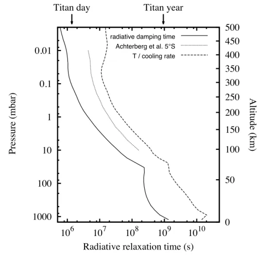
emissivity of 1.0. Radiative cooling and heating rates are then calculated on the atmospheric 364
pressure grid by differentiation of the solar and thermal fluxes. After adding the adiabatic and 365
advective cooling/heating terms in Eq. 1 to the radiative terms, the variation of temperature 366
DT at each level is calculated from Eq. 1 as Dt times the sum of these three energy terms, and 367
the process is iterated till the desired date. 368
369
4. Results
370 371
4.1 Heating and cooling rates in the stratosphere 372
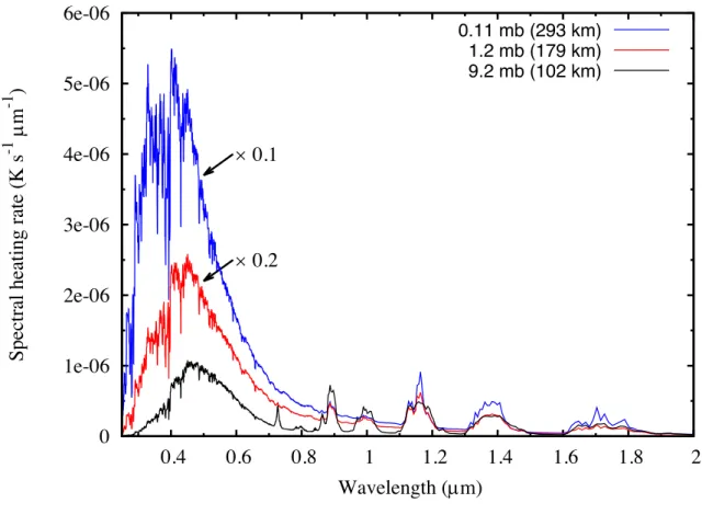
Figure 3 shows, at three different pressure levels, the spectral heating rate hl, giving the
373
wavelength dependence of the absorbed solar energy (the solar heating rate in Eq. 1 is 374
h = h
∫
λdλ ). At pressures less than ~5 mbar, heating is dominated by aerosol absorption of375
solar radiation at wavelengths below 0.8 µm, with a peak around 0.4 µm at 0.1 mbar and 0.45 376
µm at 1 mbar. At 10 mbar, the strong methane bands between 0.8 and 3.7 µm provide 377
substantial additional heating. In this region, methane and aerosol absorption provide 378
comparable contributions to the solar heating while, at deeper levels, methane absorption 379 dominates. 380 381 382 383 0 1e-06 2e-06 3e-06 4e-06 5e-06 6e-06 0.4 0.6 0.8 1 1.2 1.4 1.6 1.8 2
Spectral heating rate (K s
-1 µ m -1 ) Wavelength (µm) × 0.1 × 0.2 0.11 mb (293 km) 1.2 mb (179 km) 9.2 mb (102 km)
Figure 3: Spectral heating rate hl giving, as a function of wavelength, the contribution per
unit wavelength to the day-averaged solar heating rate at three different atmospheric levels. For clarity, hl at 0.11 mbar is multiplied by 0.1 and hl at 1.2 mbar by 0.2. The solar
heating rate is integrated from 0.25 to 3.8 µm. Insolation conditions correspond to 20°S and March 2007.
384
385
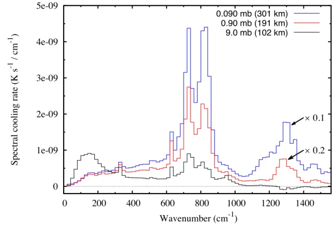
The spectral distribution of the radiative cooling rate (cs), averaged over 20-cm-1 intervals, is
386
shown in Fig. 4 at three different levels in the stratosphere. The cooling rate c in Eq. 1 is the 387
integral over wavenumber of cs: c = c
∫
σdσ . The most efficient gaseous coolers are ethane388
(820 cm-1), acetylene (730 cm-1) and, above the ~5 mbar level, methane (1300 cm-1). Note
389
that at (and below) the 9-mbar level, the methane band heats the atmosphere from above. 390
Substantial cooling in the stratosphere arises from the continuous aerosol opacity. As noted 391
earlier by Tomasko et al. (2008b), the cooling effects of gas and aerosol emission are of the 392
same order. Note, in the 9-mbar cooling rate spectrum, the contribution from the nitrile haze 393
peaking at 160 cm-1 (Anderson and Samuelson 2011).
394 0 1e-09 2e-09 3e-09 4e-09 5e-09 0 200 400 600 800 1000 1200 1400
Spectral cooling rate (K s
-1 / cm -1 ) Wavenumber (cm-1) × 0.1 × 0.2 0.090 mb (301 km) 0.90 mb (191 km) 9.0 mb (102 km)
Figure 4: Spectral distribution of the cooling rate cs, averaged over 20-cm-1 bins, giving, as
a function of wavenumber, the contribution to the radiative cooling rate at three different atmospheric levels. For clarity, cs at 0.09 mbar is multiplied by 0.1 and cs at 0.9 mbar by
395
In Fig. 5, we show the heating and cooling rate profiles calculated with our model for the 396
composition and temperature profile derived from CIRS measurements near 20°S in March 397
2007. Both profiles steadily decrease with depth, by more than 3 orders of magnitude from 398
the lower mesosphere to the lower troposphere. In the whole region 0.1-5 mbar, best 399
constrained by CIRS measurements in terms of temperature, haze and composition, the 400
heating and cooling rate profiles are remarkably similar, the former being regularly 20-35% 401
larger than the latter. The difference between them varies between 3 × 10⁻⁶ K s-1 at 0.1 mbar
402
and 2 × 10⁻⁷ K s-1 at 5 mbar. As the observed temperature variation around 2007 is less than 1 403
K year-1 (Fig. 1), i.e. < 3 × 10⁻⁸ K s-1, the energy balance equation (Eq. 1) implies that this 404
difference has to be balanced by adiabatic cooling. This leads to upward velocities decreasing 405
from 0.25 cm s-1 at 0.1 mbar to 0.09 cm s-1 at 1 mbar and 0.014 cm s-1 at 5 mbar. 406 0.01 0.1 1 10 100 1000 10-9 10-8 10-7 10-6 10-5 10-4 500 450 400 350 300 250 200 150 100 50 0 Pressure (mbar) Altitude (km) -1 20°S March 2007 Heating rate Cooling rate
407
Around 15 mbar (85 km), which corresponds to the peak of the nitrile haze, the cooling and 408
heating rates are almost equal. Just below, around 25 mbar (71 km), the heating rate exceeds 409
the cooling rate by about 70%. This region corresponds to the fall-off of the C2H6 and C2H2
410
mixing ratios due to condensation, these two gases being important infrared radiators in the 411
whole stratosphere. Below the 50-mbar level, in the troposphere, the heating rate is about 412
40% larger than the cooling rate. Note that no information from CIRS data is available using 413
the n4 CH4 band below the ~ 10-mbar level, and the temperature profile then joins the
414
Huygens/HASI in situ measurements at 10°S (Fulchignoni et al. 2005). Above the ~ 0.03-415
mbar level, the heating rate is about twice the cooling rate, which would call from Eq. 1 for an 416
upward velocity w of about 1.5 cm s-1. However, this estimation is very uncertain due to the 417
poorly known haze density in this region. 418
419
4.2 Radiative relaxation times 420
Evaluation of radiative time constants is important to investigate the response of Titan’s 421
atmosphere to various perturbations, such as the diurnal and seasonal cycles of insolation, or 422
atmospheric waves. As discussed by Flasar et al. (2014), the radiative time constant (tr) is the 423
characteristic time for radiatively damping out a small perturbation from the equilibrium state, 424
keeping unchanged all other energy terms such as solar and dynamical heating. From Eq. 1, tr 425
is formally equal to the inverse of the derivative of the cooling rate with respect to 426
temperature: 427
Figure 5: Heating (solid line) and cooling (dashed line) rate profiles calculated with our model using the temperature profile retrieved from CIRS measurements at 20°S in March 2007. The heating rate profile corresponds to day-averaged conditions and insolation parameters for March 2007.
τr(z) = 1 / ∂c(z) ∂T (z) (7) 428 429 430
However, c(z) in a given layer depends to some extent, through exchange terms, on the 431
temperature outside this layer so that the vertical shape of the assumed perturbation has to be 432
specified. We assumed here a Gaussian perturbation having a FWHM of 1 pressure scale 433
height and centered in a layer [pi:pi+1]. Doing so, ∂c(z)
∂T (z) can be calculated from Eq. 5 as a 434 0.01 0.1 1 10 100 1000 106 107 108 109 1010 500 450 400 350 300 250 200 150 100 50 0 Pressure (mbar) Altitude (km)
Radiative relaxation time (s)
Titan day Titan year
radiative damping time Achterberg et al. 5°S T / cooling rate
Figure 6: Vertical profiles of radiative relaxation time in Titan’s atmosphere. The solid line corresponds to damping out a Gaussian temperature perturbation having a full width at half maximum of one pressure scale height. The dotted line shows the radiative time constant calculated by Achterberg et al. (2011) at 5°S using the direct cooling-to-space
approximation for the radiative cooling. The dashed line represents the temperature divided by the cooling rate, following the approach of Strobel et al. (2009).
linear combination of terms in the form (Ai+1, j,k− Ai, j,k)
∂Bσk#$T ( pj)%& ∂T ( pj)
where j runs over the 435
perturbed levels with appropriate weighting. The resulting profile of tr is shown in Fig. 6 as a 436
solid line. 437
438
The radiative time constant readily increases with depth from less than 1 Titan day above the 439
0.1-mbar level to about 1 Titan year in the lowest layers of the troposphere. In the range 0.1-5 440
mbar, in which we are mostly interested here, the radiative time constant varies between 441
0.0015 and 0.02 Titan year, implying that the stratosphere can respond radiatively to the 442
seasonally-varying insolation with negligible time lag. We also made a calculation for a 443
perturbation having a twice larger FWHM (2 scale heights). The resulting time constants are 444
then ~ 25% larger in the stratosphere and ~ 60% in the troposphere below the 300-mbar level. 445
446
In Fig. 6, we also show the radiative cooling timescale calculated by Achterberg et al. (2011) 447
at 5°S using the direct cooling-to-space approximation and including opacity from CH4, C2H2
448
and C2H6. Their time constants are 4-5 times larger than those inferred in this work. A factor
449
of ~ 2 is likely due to the lack of aerosols and other gases in their calculations and the 450
remaining difference from ignoring the exchange terms, as discussed in Section 5. We also 451
plotted in Fig. 6, the ratio of temperature to cooling rate (T(z)/c(z)), which yields a simpler 452
estimate of the radiative timescale. As can be seen from Eq. 1, rather than relevant to damping 453
of a temperature perturbation, this time constant pertains to a case in which the solar heating 454
is turned off (as well as the dynamical term). This is the approach that was used by Strobel et 455
al. (2009) to compute the radiative timescale. Figure 6 shows that, doing so, the radiative 456
damping time is overestimated typically by a factor of 10. 457
4.3 Temperature profile at 6°N 459
We first compare the predictions of our seasonal radiative model, with no adiabatic 460
heating/cooling, to the temperature profile retrieved near 6°N around northern spring equinox 461
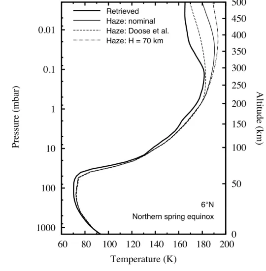
(See Section 2), a region where seasonal variations of insolation are minimal. Figure 7 shows 462
the temperature profile calculated with the three haze profiles of Fig. 2. Temperatures in these 463
models essentially differ above 200 km due to different assumptions on the vertical profile of 464
aerosol extinction. The warmest profile is associated with the largest aerosol number 465
extinction profile and vice versa, confirming that aerosol heating from scattering and 466
absorption of solar radiation dominates over their cooling effect due to thermal emission. The 467
difference between the extreme profiles increases from 7 K at 0.1 mbar to 20 K at 0.001 mbar. 468 469 0.01 0.1 1 10 100 1000 60 80 100 120 140 160 180 200 500 450 400 350 300 250 200 150 100 50 0 Pressure (mbar) Altitude (km) Temperature (K) 6°N Northern spring equinox Retrieved
Haze: nominal Haze: Doose et al. Haze: H = 70 km
470
Whatever haze profile is used, the radiative model profile is warmer than the retrieved one at 471
all levels except around 15 mbar (85 km). Note that below 5 mbar, the profile is not 472
constrained by Cassini/CIRS measurements but essentially represents the Huygens/HASI 473
profile (10°S, January 2005). To bring the calculated and observed profiles closer, it is 474
necessary to add adiabatic cooling. For our nominal haze model, we find that a constant 475
vertical velocity, expressed in pressure coordinates (1x1& = −𝜌𝑔𝑤, where r is the atmospheric 476
density), of » -1.3 Pa per Titan day up to the 0.6-mbar level, slightly decreasing in amplitude 477
at higher altitudes to reach » -1.0 Pa per Titan at 0.02 mbar, allows us to reproduce fairly well 478
the observed profile from the 0.05-mbar level down to the troposphere (Fig. 8, dashed line). 479
The largest discrepancy occurs around 15 mbar, where the model profile is 5 K colder than 480
the Huygens profile. 481
482
483
This velocity profile corresponds to an upward vertical velocity w in the range 0.03-0.05 cm 484
s-1 at 1 mbar, taking into account a 1 K uncertainty (Fig. 9), which corresponds to the
485
dispersion in our 6°N temperature profile selection (Section 2). w varies as (rg)-1 below the
486
0.6-mbar level and as (rg)-0.92 in the 0.6-0.02 mbar range. At higher levels, the velocity is set
487
so that it varies as (rg)-0.1 from 0.02 to 0.01 mbar, and as (rg)0.35 above (Fig. 9). The
488
approximate constancy of 1x below the 0.02-mbar level suggests only weak divergence of 489
0.01
0.1
1
10
100
1000
60
80 100 120 140 160 180 200
500
450
400
350
300
250
200
150
100
50
0
Pressure (mbar) Altitude (km)Temperature (K)
6°N Northern spring equinox RetrievedModel w = 0 Model with w
Figure 8: Comparison of a temperature profile retrieved from Cassini/CIRS measurements around 6°N and northern spring equinox (thick solid line) with two radiative model profiles using the nominal haze model. The thin solid line shows the case with no additional adiabatic heating (same as in Fig. 7). The dashed line shows a model with a constant velocity below the 0.6-mbar level, when expressed in pressure coordinates, equal to -1.3 Pa / Titan day, decreasing to -1.0 Pa / Titan day at 0.02 mbar and -0.5 Pa / Titan day at 0.01 mbar (Fig. 9).
the upward flow in the stratosphere, while the decrease of 1x1& at higher levels implies stronger 490
divergence, i.e. horizontal poleward motion. However, this conclusion is not firm due 491
uncertainties in the haze profile. It still holds if we use the upper limit for the haze density (“H 492
= 70 km” case) but not for the lower limit (Doose et al. profile), in which case a strong 493
decrease of 1x1& above the » 1 mbar level is required to reproduce the 6°N temperature profile 494
(Fig. 9). 495
496
497
4.4 Seasonal variations of temperature at 1 mbar 498 0.001 0.01 0.1 1 10 100 1000 0.01 0.1 1 10 Pressure (mbar)
ρgw (Pa / [Titan day])
0.001 0.01 0.1 1 10 100 1000 10-5 10-4 10-3 10-2 10-1 100 101 Pressure (mbar) Vertical velocity w (cm s-1)
Figure 9: Upward velocity profile used to model the temperature profile retrieved at 6°N around equinox, given in pressure units per Titan day (left panel) and in cm s-1 (right panel). The black line corresponds to the model with the nominal haze profile that yields the best fit of the temperature profile (Fig. 8), while the red line corresponds to the Doose et al. profile and the blue line to the “H = 70 km” haze profile shown in Fig. 2. The grey area around the best fit velocity profile corresponds to a temperature uncertainty taken as the standard deviation of our 6°N temperature profile selection given in Section 2.
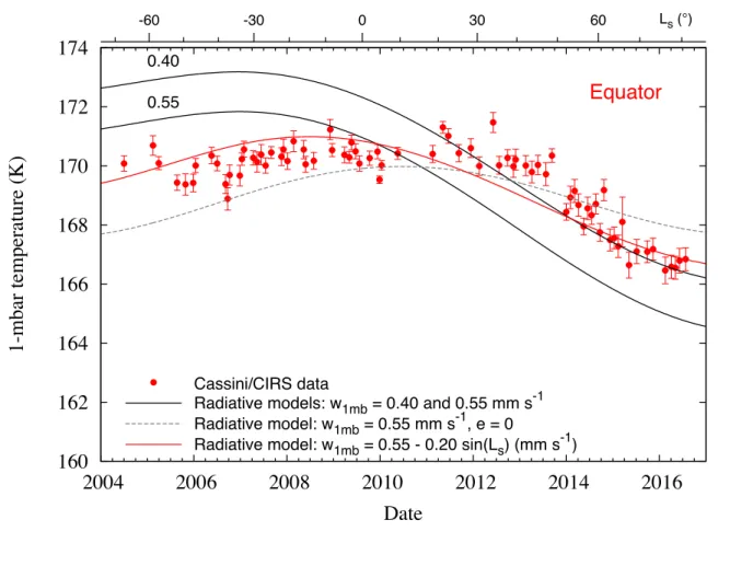
We first investigate here the variations of temperatures at 1 mbar derived from Cassini/CIRS 499
in the equatorial region from 2004 to 2016 (Fig. 1). Figure 10 shows our model predictions 500
using a constant upward velocity of 0.040 cm s-1 at 1 mbar as derived above around 6°N near
501
northern spring equinox. This model predicts a ~7 K drop between pre-equinox (2006-2008) 502
and 2016. This variation is due to Saturn’s eccentricity of 0.054, which modulates the 503
distance to the Sun and thus the solar flux striking the Saturn system. A model with zero 504
eccentricity (dashed line in Fig. 10) shows a shallow maximum around mid 2010 and similar 505
temperatures in 2006 and 2016. In contrast, the model accounting for the orbital eccentricity 506
predicts a maximum around 2007, between the perihelion (July 2003) and the equinox 507
(August 2009), followed by a decrease due to the increasing distance with the Sun. In fact, 508
while the temperatures after 2012 are then correctly reproduced by this model, the contrast 509
between pre-equinox and 2016 (~7 K) is even larger than the observed value of ~4 K. 510
Increasing the vertical velocity in the model uniformly shifts the calculated temperatures and 511
does not help to reduce the contrast (Fig. 10). To better reproduce the observations, a 512
modulation of the vertical velocity, i.e. of the adiabatic cooling, is required. We chose to do 513
so by simply adding a sine function of the heliocentric longitude Ls to the velocity, which then
514
becomes: 515
𝑤 𝑝 = 𝑤{ 𝑝 + 𝑤| 𝑝 sin 𝐿v (8)
516
At the 1-mbar level, wc = 0.055 cm s-1 and wm = 0.020 cm s-1 allows us to reproduce relatively
517
well the observed variation (red line in Fig. 10). The vertical velocity at 1 mbar then varies 518
seasonally between 0.035 and 0.075 cm s-1 but is always positive (upward), meaning 519
dynamical cooling of the equatorial region all year through. Note that the vertical profile of wc
520
used here and shown in Fig. 11 differs somewhat from those used at 6°N in Section 4.3 521
because it was adjusted to better match the temperatures at 0.2, 0.5, 1, 2 and 4 mbar retrieved 522
by Achterberg et al. (in preparation) and shown in Section 4.6. 523
524 525 160 162 164 166 168 170 172 174 2004 2006 2008 2010 2012 2014 2016 1-mbar temperature (K) Date Equator 0.40 0.55 0 30 -30 -60 60 Ls (°) Cassini/CIRS data
Radiative models: w1mb = 0.40 and 0.55 mm s-1 Radiative model: w1mb = 0.55 mm s-1, e = 0
Radiative model: w1mb = 0.55 - 0.20 sin(Ls) (mm s-1)
Figure 10: Time variation of 1-mbar temperatures in the equatorial region are compared with predictions from our seasonal radiative model. Solid lines represent models with constant-with-time upward velocity profiles having w(1 mbar) = 0.040 and 0.055 cm s-1. The dashed line represents a model with w = 0.055 cm s-1 and the orbital eccentricity set to zero. The red line represents a model with a seasonally-varying vertical velocity profile: w(1 mbar) = 0.055 – 0.020 sin(Ls) cm s-1, where Ls is the heliocentric longitude.
526
527
We then applied our model to latitudes 30°N and S where seasonal variations of insolation are 528
more pronounced. Figure 12 shows the predicted variations of temperature at 1 mbar over a 529
full Saturnian year (29.46 years), using a constant-with-time upward velocity profile (with 530
w = 0.055 cm s-1 at 1 mbar). Such a model predicts large variations of temperature as a
531
response to the seasonally-varying insolation with peak-to-peak amplitudes of 33 K at 30°S 532
and 19 K at 30°N. The amplitudes are stronger in the southern hemisphere than in the 533
northern due to the orbital eccentricity, the perihelion occurring less than a year before 534
southern summer solstice. Clearly, the predicted variations are much stronger than observed 535 0.001 0.01 0.1 1 10 100 1000 10-2 10-1 100 101 10-5 10-3 10-1 10 Pressure (mbar)
ρgw (Pa / [Titan day]) Vertical velocity w (cm s-1)
Figure 11: Thick solid lines: upward velocity profile used to model the temperature profile retrieved at 6°N around equinox (Fig. 8), given in pressure units per Titan day (black) and in cm s-1 (red). Thin solid lines: year-averaged upward velocity profile wc used to model the seasonal temperature variations at the equator as retrieved by CIRS (Figs. 10 and 15). Thin dashed lines: amplitude of the sine term of this upward velocity profile wm. See Eq. 8. Note that wc and wm are constrained from CIRS observations only from 0.2 to 4 mbar.
by Cassini since 2004 (Fig. 12). Most noticeable in this comparison is the observed decrease 536
of the 1-mbar temperature since 2013 at 30°N, which is at odds with the increase predicted by 537
the radiative model as a result of increasing insolation. This behavior can only be explained 538
by an increase of the dynamical cooling with time at this latitude. More generally, the 539
observed variations at 30°N and S point to dynamics acting to counterbalance the seasonal 540
variations in the solar heating. This means dynamical heating, or reduced cooling, in winter 541
and enhanced dynamical cooling in summer. To model this pattern in a simple way, we 542
proceeded as above and modulated the vertical velocity in the form of Eq. 8. The best fits to 543
the data that we obtained are shown in Figs. 13-14 with the corresponding values of wc and
544
wm given in Table 1. As can be seen, this simple model is able to reproduce the observed
545
variations relatively well. 546
547
Table 1. Model parameters for the vertical velocity profile1
548 Latitude wc (1 mbar) (cm s-1) wm (1 mbar) (cm s-1) Pressure range (mbar) ac am Equator +0.055 -0.020 < 0.01 -0.40 -0.40 30°N +0.063 +0.075 0.01-0.025 0.20 0.20 30°S +0.053 -0.105 0.025-0.4 0.45 0.30 0.4-1 1.0 0.60 > 1 1.2 0.90
1: upward velocity is modeled as 𝑤 𝑝 = 𝑤
{ 𝑝 + 𝑤| 𝑝 sin 𝐿v, and wc (resp. wm) varies as 549
(r𝑔)X}~ (resp. (r𝑔)X}•) in a given pressure range.
550 551
552 553 554 555 140 145 150 155 160 165 170 175 180 1990 1995 2000 2005 2010 2015 1-mbar temperature (K) Date Radiative model w1mb = 0.55 mm s-1 Cassini/CIRS data • • • Equator 30°N 30°S 160 162 164 166 168 170 172 174 2004 2006 2008 2010 2012 2014 2016 1-mbar temperature (K) Date 30°N 0 30 -30 -60 60 Ls (°) Cassini/CIRS data 30°N Radiative model: w1mb = 0.55 mm s-1
Radiative model: w1mb = 0.63 + 0.75 sin(Ls) (mm s-1)
Figure 12: Time variation of 1-mbar temperatures at 0°, 30°N and 30°S predicted by the seasonal radiative model using a constant-with-time upward velocity profile with w(1 mbar) = 0.055 cm s-1. Data retrieved from Cassini/CIRS measurements (Fig. 1) are overplotted for comparison.
557 558 559 560 561 562
4.5 Seasonal variations of temperature at other levels 563
In Section 4.4, we focused on the 1-mbar level, which is the region best constrained by 564
Cassini/CIRS observations in terms of haze properties and temperature, and we have tuned 565
our model to best reproduce the data at this level. In this section, we extend our modelling up 566
to 0.2 mbar and down to 4 mbar, where temperature information is also available (Fig. 15). To 567
do so, we used a vertical velocity profile w(p) varying as (rg)-a in a given pressure range as
568
indicated in Table 1 and shown in Fig. 9 at the equator. As we intend to keep a smooth 569
variation for w(p), we did not try to match exactly the average temperature at a given pressure 570 160 162 164 166 168 170 172 174 2004 2006 2008 2010 2012 2014 2016 1-mbar temperature (K) Date 30°S 0 30 -30 -60 60 Ls (°) Cassini/CIRS data 30°S Radiative model: w1mb = 0.55 mm s-1
Radiative model: w1mb = 0.53 - 1.05 sin(Ls) (mm s-1)
Figure 13: Time variation of 1-mbar temperatures at 30°N predicted by the seasonal radiative model are compared with data retrieved from Cassini/CIRS measurements (Fig. 1). Black line: constant-with-time vertical velocity; colored line: vertical velocity varying with solar longitude (see parameters in Table 1).
level apart from that at 1 mbar. We then have typical discrepancies of ±3 K on the average 571
temperatures which may be due to uncertainties in our haze model above ~0.4 mbar (Fig. 7) 572
and possibly systematic uncertainties in the temperature retrievals below ~2 mbar. We are 573
therefore more interested here in the seasonal variations of temperature at a given level than 574
in their absolute mean values. 575 145 150 155 160 165 170 175 180 185 2004 2006 2008 2010 2012 2014 2016 30°S 145 150 155 160 165 170 175 180 185 2004 2006 2008 2010 2012 2014 2016 Eq 145 150 155 160 165 170 175 180 185 2004 2006 2008 2010 2012 2014 2016 Date 30°N 0.2 0.5 1 2 4
577 578 579 580
In Fig. 15, we show the seasonal variations of temperature predicted by our model for 581
different pressure levels at 0, 30°N and 30°S. In these “best-fit” models, the vertical variation 582
of the constant and sine components of the velocity profile were chosen to reproduce 583
satisfactorily the observed seasonal variations at the three latitudes simultaneously (only one 584
set of parameters for all latitudes, given in Table 1). On the other hand, the velocity terms wc 585
and wm at 1 mbar were adjusted at each latitude to best reproduce the seasonal variations at 586
this level, as discussed in Section 4.4. The CIRS-derived variations are overall fairly well 587
reproduced except noticeably at 4 mbar where the steady decrease of temperature at the 588
equator and at 30°N before equinox (2009) is not predicted by the model. 589 590 591 592 -1 -0.5 0 0.5 1 1.5 -180 -150 -120 -90 -60 -30 0 30 60 90 120 150 180 2000 2005 2010 2015 2020 2025
1-mbar upward velocity (mm s
-1 ) Ls (°) 1 mbar w1mb = 0.55 - 0.20 sin(Ls) (mm s-1) w1mb = 0.63 + 0.75 sin(Ls) (mm s-1) w1mb = 0.53 - 1.05 sin(Ls) (mm s-1) Equator 30°N 30°S
Figure 15: Time variation of temperatures at 0.2, 0.5, 1, 2 and 4 mbar predicted by the seasonal radiative model (colored lines) are compared with data retrieved from
Cassini/CIRS measurements at 30°S, equator and 30°N. In this model, the vertical velocity varies as an affine function of sin Ls (see parameters in Table 1).
Figure 16: Time variation of the 1-mbar model upward velocity at 0°, 30°N and 30°S as a function of heliocentric longitude (lower scale) and year (upper scale).
The seasonal variation of the model velocity profile w at 1 mbar is shown in Fig. 16 for the 593
three latitudes. The seasonal variation at other pressure levels can be obtained from the 594
parameters in Table 1. The vertical dependence of the two components (wc and wm in Eq. 8) is 595 illustrated in Fig. 11. 596 597 5. Discussion 598 599
5.1 Heating and cooling rates 600
Tomasko et al. (2008b) computed the solar heating rate at Huygens probe-landing latitude, 601
averaged over longitude, using the haze model derived from DISR measurements by 602
Tomasko et al. (2008c) and methane absorption coefficients simultaneously derived from 603
DISR measurements (Tomasko et al. 2008a). The solar heating rates we derived at 20°S in 604
March 2007 do not differ from those of Tomasko et al. by more than ±25% in the range 10-605
170 km. The largest differences occur at 10 and 170 km where our heating rate is some 20% 606
larger and near 90 km where our heating rate is 25% smaller. We regard these differences as 607
acceptable given the difference in the haze model, which was recently updated by Doose et al. 608
(2016), and in the methane absorption, which we calculate using the ab initio TheoReTS 609
database (Rey et al. 2017). 610
611
Cooling rates corresponding to the temperature, gas and haze profiles derived from Huygens 612
and Cassini/CIRS data were also calculated by Tomasko et al. (2008b). Our cooling rate 613
profile agree with theirs to within ±20% in the whole altitude range 10-400 km, with the 614
maximum discrepancy occurring near 10 km (ours is 20% smaller) and 70 km (ours is 20% 615
larger). 616
Comparing the heating and cooling rates calculated at the Huygens landing site, Tomasko et 618
al. (2008b) concluded that the former exceeds the latter by a maximum of 0.5 K per Titan day 619
near 120-130 km and that the excess decreases strongly below and above this altitude. At 125 620
km, we derive 0.4 K / Titan day, in good agreement with Tomasko et al. Below this altitude, 621
we also find that the net radiative heating minus cooling rate decreases rapidly, e.g. 0.07 K / 622
Titan day at 70 km and 0.02 K / Titan day at 50 km, quite similar to Tomasko et al.’s results. 623
On the other hand, we do not infer any decrease of this net radiative heating minus cooling 624
above 120-130 km, but instead a regular increase up to 3 to 4 K per Titan day at 250-300 km. 625
We note however that the decrease at higher altitudes invoked by Tomasko et al. is very 626
uncertain given the large uncertainties in their haze model above 140 km, the altitude where 627
the Huygens probe began measurements. Our haze model is also uncertain above ~200 km, 628
where the net radiative heating minus cooling rate reaches ~2 K per Titan day. 629
630
We can also compare our calculations with the General Circulation Model (GCM) of 631
Lebonnois et al. (2012, Fig. 10). At 20°S, their annual average of the solar heating rate is 632
almost twice as large as ours at 90-100 km, 50% larger at 60 km and 30% larger at 50 km. 633
These differences likely originate from differences in the haze model, that in Lebonnois et 634
al.’s GCM being coupled with the 3-dimensional circulation and not imposed from 635
observational constraints. More significant for our model comparison may be the ratio of 636
dynamical cooling to total (radiative plus dynamical) cooling, also equal to radiative solar 637
heating on an annual average basis. At 6°N, where seasonal modulation is minimum, this ratio 638
can be determined from Fig. 10 of Lebonnois et al. at 85 and 66 km as approximately 18% 639
and 25% respectively. Using the vertical velocity of 1.1 Pa / Titan day that we inferred in 640
Section 4.3 at this latitude and the yearly-averaged solar heating rate from our model, we 641
obtain ratios of 17% at 85 km and 28% at 66 km, in excellent agreement with Lebonnois et 642
al.’s GCM outputs. Lebonnois et al. (2012) do not provide information to compare results 643 above 100 km. 644 645
5.2 Radiative relaxation times 646
In Section 4.2, we calculated the radiative time constant (𝜏9) corresponding to damping a 647
temperature perturbation relative to the radiative equilibrium state, having a FWHM of one 648
pressure scale height (Fig. 6). This time constant depends somewhat on the width of the 649
temperature perturbation and doubling the width increases its value by 25% in the 650
stratosphere. Strobel et al. (2009) provided another estimate of a radiative timescale by 651
dividing temperature by the cooling rate, which actually corresponds to the time decay of 652
temperature when the solar heating is turned off starting from the radiative equilibrium state. 653
While this timescale may be appropriate to investigate diurnal variations of temperature, it 654
strongly overestimates the time constant associated with the damping of small temperature 655
perturbations around the radiative equilibrium state such as those caused by gravity waves or 656
moderate seasonal variations of insolation. Figure 6 shows that our time constant 𝜏9 is about a 657
factor of 10 smaller than the timescale of Strobel et al., which is important to evaluate 658
correctly the response of the atmosphere to e.g. seasonal forcing or planetary waves. For 659
example, our calculation indicates that 𝜏9 exceeds 1 Titan year only in the first 7 km of 660
Titan’s atmosphere while Strobel et al.’s estimation would predict that it happens at all 661
altitudes below 76 km. In the upper troposphere and tropopause region, 30-60 km, 𝜏9 is 0.25 662
to 0.3 Titan year, which allows for non-negligible seasonal variations of temperature in 663
contrast to expectations using Strobel et al.’s simpler formulation. In the stratosphere, above 664
100 km (p < 10 mbar), 𝜏9 is less than 0.03 Titan year (25 Titan days), so that significant 665
seasonal temperature variations with almost no phase lag are expected. 666