HAL Id: hal-00513255
https://hal.archives-ouvertes.fr/hal-00513255
Submitted on 1 Sep 2010HAL is a multi-disciplinary open access archive for the deposit and dissemination of sci-entific research documents, whether they are pub-lished or not. The documents may come from teaching and research institutions in France or
L’archive ouverte pluridisciplinaire HAL, est destinée au dépôt et à la diffusion de documents scientifiques de niveau recherche, publiés ou non, émanant des établissements d’enseignement et de recherche français ou étrangers, des laboratoires
To cite this version:
Samuela Pasquali, Jerome K Percus. Mean Field and the Confined Single Homopolymer. Molecular Physics, Taylor & Francis, 2009, 107 (13), pp.1303-1312. �10.1080/00268970902776740�. �hal-00513255�
For Peer Review Only
Mean Field and the Confined Single Homopolymer
Journal: Molecular Physics Manuscript ID: TMPH-2008-0340.R1 Manuscript Type: Full Paper
Date Submitted by the
Author: 22-Jan-2009
Complete List of Authors: Pasquali, Samuela; Institut de Biologie Physico-Chimique (IBPC), Laboratoire de Biochimie Théorique
Percus, Jerome; New York University, Physics and Courant Institute Keywords: confined polymers, folding, long-range interactions
Note: The following files were submitted by the author for peer review, but cannot be converted to PDF. You must view these files (e.g. movies) online.
For Peer Review Only
Mean Field and the Confined Single Homopolymer
S. Pasquali1, J.K. Percus2
1Laboratoire de Physico-Chime Th´eorique, UMR Gulliver CNRS-ESPCI 7083,
10 rue Vauquelin, 75231 Paris Cedex 05, France.
2Courant Institute and Physics Department NYU, 251 Mercer St. New York, NY 10012
(Dated: January 22, 2009)
We develop a statistical model for a confined homopolymeric chain molecule based on a monomer grand ensemble representation. The molecule is subject to a confining external field, a backbone interaction, and an attractive interaction between any pair of monomers. An exact minimum principle for the thermodynamics of the backbone in an external field is obtained, and a controlled mean field approximation results in a modified minimum prin-ciple from which relevant physical quantities such as monomer density can be found. We explore the limit in which the chain is subject to tight confinement, and make a preliminary investigation of a prototypical system.
PACS numbers: 05.20.Gg, 82.35.Lr,
87.15.A-I. INTRODUCTION
The question of how linear macromolecules like proteins fold inside a cavity is of great biological relevance. Indeed it is now recognized that large proteins are not capable of correctly folding in the crowded cell’s environment, where the volume fraction occupied by macromolecules can be of the order of 20 − 30% [1], but they need some kind of cavities to fold, where they are isolated from the rest of the cell’s environment, and can avoid interactions with other molecules which would cause misfolding and aggregation [2]. Moreover, in vitro experiments where the effects of confinement on the thermodynamics of protein folding were directly monitored, seem to indicate that confinement increases the stability of the native states [3].
The simplest representation of biopolymers under confinement, is one where the molecule is modeled by a classical chain under an external field. The work presented in this paper aims at the development of a consistent and well grounded perturbative approach to the theory of confined polymer folding. Studies of polymers have of course been extensive, and useful relationships be-tween polymer melts and fluids established [4], as well as bebe-tween single polymers and fluids. This paper represents an initial investigation, aimed at understanding which concepts borrowed from bulk fluid studies [5, 6] still remain relevant in a polymer setting. The classical theory of fluids
3 4 5 6 7 8 9 10 11 12 13 14 15 16 17 18 19 20 21 22 23 24 25 26 27 28 29 30 31 32 33 34 35 36 37 38 39 40 41 42 43 44 45 46 47 48 49 50 51 52 53 54 55 56 57 58 59 60
For Peer Review Only
in thermal equilibrium is a highly developed discipline. Along with specific physically motivated approximations have come tools of more general validity and utility.
Our focus will be on a single polymer chain confined by external forces, and to minimize the needed information input, on single homopolymers. We will also attend in the main to idealized models in which the polymer is simply a chain of unit monomers of a few degrees of freedom, but will indicate how this restriction can be rewardingly removed, on the way to a realistic polymer representation.
We will aim at both analytic simplicity and reasonable suitability for the ultimately necessary computational procedures. For the former, we will work in a “monomer grand-ensemble”[7, 8] in which the number of monomers per polymer is distributed, but will show that this need not be a drawback. For the latter, we will favor minimum principles to be able to better control computations. This does restrict the category of systems to be studied e.g. to purely attractive pair interactions, and will be generalized in later work, soon to be reported, as such restrictions are removed.
II. THE REFERENCE SYSTEM
The statistical mechanics of a free classical chain molecule, interpreted as a random walk is an old, old topic, although less attention has been paid to the effect of a structured external field, in part because the formal simplification afforded by translation invariance is then not available. In this case, the next neighbor pair energy then depends separately on the locations of each of the monomers in the pair, rather than on just their separation (in the point monomer model). We will tackle this problem by first (section II A) concealing the discreteness of the monomer population number, and then (section II B) concealing the inherent required inversion of the pair Boltzmann factor kernel.
A. Notation
Let us be a bit more explicit. We have in mind an ordered chain of N equivalent monomers, the jth being specified by its degrees of freedom r
j. The order is maintained by a symmetric
next neighbor interaction potential of Boltzmann factor w(ri, ri+1), depending of course on the
inverse temperature β. Any two monomers can also interact via an interaction Boltzmann factor e(ri, rj) = exp(−βφ(ri, rj)) and, crucially for the applications we have in mind, the polymer is
2 3 4 5 6 7 8 9 10 11 12 13 14 15 16 17 18 19 20 21 22 23 24 25 26 27 28 29 30 31 32 33 34 35 36 37 38 39 40 41 42 43 44 45 46 47 48 49 50 51 52 53 54 55 56 57 58 59 60
For Peer Review Only
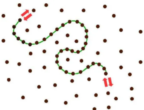
FIG. 1: Graphical sketch of the monomer bath. The chain is in grand canonical equilibrium with a bath of inert monomers.
constrained by an external potential u(ri).
It is now convenient to imagine that the homopolymer in question is both in thermal equilibrium and in number equilibrium, i.e. that it is the result of monomer addition and absorption from a bath of non-interacting monomers (figure 1). The reaction equilibrium is analogous to that of the grand canonical ensemble for a fluid, but with a significant difference. Suppose that Q(m) is
the monomer canonical partition function in its center of mass coordinate system, Q(p)N of the N -monomer polymer (N ≥ 1, to recognize an object as a polymer). Then if the full system contains N′ monomers, N of which are bound together, in a volume V , the full system partition function
will be: QtotN′ = X N ≥1 (V Q(m))N′−N (N′− N )! Q (p) N . (1)
Since the monomers in the absence of a polymer would have a partition function:
Q(m)N′ =
(V Q(m))N′
N′! (2)
that attributed to the polymer will take on the form:
Ξ(p)[ζ0] = lim N′→∞,N′/V fixed N′! (V Q(m))N′Q tot N′ (3) = X N ≥1 ζ0NQ(p)N , where ζ0 = (N′/V )/Q(m). (4)
The obvious analogy with a fluid grand partition function (with the weight 1/N ! excised) will be very useful indeed.
The computation of Ξ(p)(ζ0), which generates all thermodynamics and expectations in a thermal
ensemble, is of course too general to be explicitely solvable, except in very special circumstances.
3 4 5 6 7 8 9 10 11 12 13 14 15 16 17 18 19 20 21 22 23 24 25 26 27 28 29 30 31 32 33 34 35 36 37 38 39 40 41 42 43 44 45 46 47 48 49 50 51 52 53 54 55 56 57 58 59 60
For Peer Review Only
Let us therefore start with the evaluation of Ξ(p)(ζ0) for what may be regarded as the backbone of
the polymer, that in which the arbitrary pair mutual interaction φ(ri, rj) is set equal to zero. In
this case, we have at once:
ζ0NQ(p)N =
Z
ζ(r1)w(r1, r2)ζ(r2) . . . ζ(rN −1)w(rN −1, rN)ζ(rN)drN (5)
where ζ(r) = ζ0e−βu(r)= eβµ(r)
or regarding w(r, r′) as the kernel of an integral operator w, ζ(r)δ(r − r′) as that of the diagonal
operator ζ, and the symbol |1i denoting the vector whose components are 1,
Ξ(p)[ζ] = h1|(ζ−1− w)−1|1i, (6)
subject of course to convergence of the series (4). The corresponding “grand potential” is:
Ω(p)[ζ] = −1
β lnh1|(ζ
−1− w)−1|1i (7)
and as an immediate consequence the monomer density is given by
n(r) = −βζ(r) δ δζ(r)Ω
(p)[ζ] (8)
= h1|(ζ−1− w)−1|rihr|(ζ−1− w)−1|1iζ−1(r)/h1|(ζ−1− w)−1|1i (9)
The absence of the statistical weight 1/N ! in (4) suggests an unusually broad distribution of monomer number N about its mean, in the ensemble. In Appendix A, we examine the form of this distribution, its consequences, and the nature of required correction terms.
B. Minimum Principle
Expression (7) for the backbone grand potential is very concise, but it requires the inversion of an integral operator, ζ(−1)− w, and so is technically non-trivial, although computationally not a great impediment. More importantly, it makes unfeasible the direct use of (7) as potential building block for the full interacting system. Fortunately, (7) can be constructed, making use of a minimum principle in which no such inverses appear. Doing so depends upon the fact that if K is positive semidefinite, and a and ψ are arbitrary, then according to the Schwartz inequality we have
ha|K−1|aihψ|K|ψi = hK−1/2a|K−1/2aihK1/2ψ|K1/2ψi (10)
≥ hK−1/2a|K1/2ψi2 = ha|ψi2, (11)
so that ha|K−1|ai ≥ ha|ψi2/ < ψ|K|ψi. Then indeed
Maxψ
ha|ψi2
hψ|K|ψi = ha|K
−1|ai atKψ = hψ|K|ψi
ha|ψi a, (12) 2 3 4 5 6 7 8 9 10 11 12 13 14 15 16 17 18 19 20 21 22 23 24 25 26 27 28 29 30 31 32 33 34 35 36 37 38 39 40 41 42 43 44 45 46 47 48 49 50 51 52 53 54 55 56 57 58 59 60
For Peer Review Only
βΩ(p)[ζ] = M inψh
lnhψ|ζ−1− w|ψi − 2 lnh1|ψii. (13)
The representation (13), it must be emphasized, is exact. There is no explicit inverse contained therein, and this indeed allows it to be used as a first step in analysis of the backbone with non-neighbor pair forces.
III. THE MEAN FIELD STRATEGY
A. Exact Results
Having the backbone of the polymer in an external field potentially under control, we now approach our real objective: to find the effect of mutual interactions, φ1(r, r′), between any two
monomers at r and r′. The most common leading estimate in such situations, termed mean field,
is one in which the mean value of the sum of pair interactions acting on a given unit is taken as an additional external field. This acts self-consistently on each unit, and so control of the non-interacting system then suffices. For classical fluids, Widom’s insertion theorem [9] tells us that if the calculation is done instead for each member of the ensemble - fluctuations hence automatically included - and then averaged over the ensemble, it becomes exact in the sense that
n(r) = heβ(µ(r)−Rφ1(r,r′)ˆn(r′)dr′)i (14) where ˆ n(r) =X i δ(r − ri) (15)
is the microscopic, per configuration, particle density. Mean field thus amounts to replacing ˆn(r′)
by hn(r′)i = n(r′). Carrying out corrections however leads to questions about the pair distribution,
which can get quite involved. For our purposes, another exact representation is preferable, in which the interaction is replaced by a suitable average over an equivalent fluctuating external field. This is of very general validity, but it applies rigorously only to the additions of purely attractive (negative definite) pair forces, which certainly can distort local properties of a real system. In the case of a polymer backbone, which already includes next neighbor pair forces, this assumption is not lethal, and we can anticipate a reasonable representation of global structure. Suppose then that, quite generally, we set φ1(r, r′) = −φ(r, r′) (16) 3 4 5 6 7 8 9 10 11 12 13 14 15 16 17 18 19 20 21 22 23 24 25 26 27 28 29 30 31 32 33 34 35 36 37 38 39 40 41 42 43 44 45 46 47 48 49 50 51 52 53 54 55 56 57 58 59 60
For Peer Review Only
for convenience (φ is now positive definite as a continuous matrix) and imagine that φ is added to a reference system all of whose properties are known.
Ξ[µ, φ] = X N Z . . . Z W0(N )(rN, µ)e β 2 P′ i,jφ(ri,rj)drN (17) = X N Z . . . Z W0(N )(rN, µ)e−β2P iφD(ri)e β 2 P i,jφ(ri,rj)drN (18) = X N Z . . . Z W0(N )(rN, µ)e−β2 P iφD(ri)e β 2 R R ˆ n(r)φ(r,r′)ˆn(r′)drdr′ drN (19) whereP′
omits the i = j contribution, φD is the diagonal part of the matrix φ(ri, rj).
The device of Kac, Siegert, Hubbard and Stratonovich [10–13] is to represent the Gaussian in (17) (in obvious notation) as a functional Laplace transform
eβ2n·φˆˆ n = Z e−β2v·φ−1v e−βv·ˆnDv / Z e−β2v·φ−1v Dv (20) = Z e−βPiv(ri)e− β 2v·φ−1vDv / Z e−β2v·φ−1vDv (21) Since P N R . . .R W0(N )(rN, µ)drN = Ξ
0[µ], eq.(17) can thereby be rewritten as
Ξ[µ, φ] = Z Ξ0[µ −1 2φD− v]e −β2v·φ−1v Dv / Z e−β2v·φ−1vDv (22)
with a possible interpretation that the interaction −φ has been replaced by an ensemble average over a fluctuating external field v(r), serving as a sort of graviton shuttling back and forth between units, and in fact, particle configuration space has now been transformed to field space. The physical interpretation is comfortable, but more importatntly, it leads to a new method of evaluation as well, and applies to fluids, polymers,....
The kernel of (22) is a Boltzmann factor in field space, and so we may define a field average as
hhG[v]ii = Z G[v]Ξ0[µ − 1 2φD − v]e −β2v·φ−1v Dv /Ξ[µ, φ] (23)
A very suggestive consequence of this notation follows from the observation that for the density n(r), n(r) = 1 Ξ[µ, φ] δ δβµ(r)Ξ[µ, φ] (24) = − Z δ δβµ(r)Ξ0[µ − 1 2φD− v]e −β2v·φ−1v Dv /Ξ[µ, φ] Z e−β2v·φ−1v Dv, (25)
or integrating by parts in v-space (assuming the absence of boundary terms)
n(r) = − Z φ−1v(r)Ξ0[µ − 1 2φD− v]e −β2v·φ−1v Dv /Ξ[µ, φ] Z e−β2v·φ−1v Dv (26) = −φ−1hhv(r)ii, (27) 2 3 4 5 6 7 8 9 10 11 12 13 14 15 16 17 18 19 20 21 22 23 24 25 26 27 28 29 30 31 32 33 34 35 36 37 38 39 40 41 42 43 44 45 46 47 48 49 50 51 52 53 54 55 56 57 58 59 60
For Peer Review Only
identifying −φn(r) as the “mean field” hhv(r)ii. Eq(27) is exact, but depends very much on the details of the system under study e.g. in (26). Exact calculations in function space are out of the question, and so it is the approximate evaluation of of hhv(r)ii that we must attend to.
B. A Mean Field Approximation
There are any number of ways of setting up approximation sequences for the evaluation of hhv(r)ii. We will adopt one which is fairly obvious in the context of (22) and (26), with the great advantage of a very pictorial leading order - still appearing as a minimum principle - and a physically transparent first order. It goes as follows. If the field Boltzmann factor of (23) is sharply peaked about a function ¯v(r), than of course (27) becomes simply
n(r) = −φ−1¯v(r), (28)
and the field ¯v must now satisfy (Ω is again the grand potential −β1ln Ξ) δ δ¯v(r) µ Ω0[µ −1 2φD− ¯v] ¶ +1 2¯v · φ −1v = 0,¯ (29) or simply n0(r|µ − 1 2φD− ¯v) = −φ −1v(r),¯ (30)
the unsurprising result (comparing with (28)) that n(r) is equal to the “bare” density n0 in the
presence of ¯v, to within an additional shift of 12φD. But in addition, we now have in leading order
approximation the very explicit
Ω1(µ, φ) = Ω0[µ − 1 2φD− ¯v] + 1 2¯v · φ −1¯v (31)
which, since (29) represents the minimization of the kernel of (24), takes the variational form
Ω1(µ, φ) = MinvΩ0[µ −1
2φD− v] + 1 2v · φ
−1v. (32)
Furthermore, consistency is established by noting that by virtue of (32), Ω1 of (31) implies
n(r) = − δΩ1
δµ(r) = −φ
−1v(r),¯ (33)
reproducing (28).
To apply (32) to the single homopolymer under discussion, we need only insert (13), serving as Ω0, into (32). We then have
βΩ1[µ, φ] = Minv,ψ ·β 2v · φ −1v − 2 lnh1|ψi + lnhψ|e−β(µ′−v) − w|ψi ¸ (34) 3 4 5 6 7 8 9 10 11 12 13 14 15 16 17 18 19 20 21 22 23 24 25 26 27 28 29 30 31 32 33 34 35 36 37 38 39 40 41 42 43 44 45 46 47 48 49 50 51 52 53 54 55 56 57 58 59 60
For Peer Review Only
where µ′(r) = µ(r) − 12φD(r). Eq. (34) can be simplified by finding and eliminating the field ψ,
and replacing v by −φn. To do so we observe that
0 = δΩ1 δv = φ
−1v + e−β(µ′−v)
ψ2 /hψ|e−β(µ′−v)− w|ψi (35)
Integrating over the implicit r, with N =R
n(r)dr, then N = hψ|e −β(µ′−v) |ψi hψ|e−β(µ′−v)− w|ψi, (36) reducing (35) to n = N e−β(µ′−v)ψ2/hψ|e−β(µ′−v)|ψi (37)
Since (37) is homogeneous of degree 0 in ψ, we are free to adopt the normalization
hψ|e−β(µ′−v)|ψi = N (38)
converting (37) to
n = e−β(µ′−v)ψ2 (39)
(leading back to (38)), and consequently replace (34) by the simple
βΩ1[µ, φ] = Minn ·β 2n · φn − 2 lnh1|n 1/2eβ2(µ′+φ·n) i + lnhn1/2|³I − eβ2(µ′+φ·n)we β 2(µ′+φ·n) ´ |n1/2i ¸ . (40) appearing as a µ-dependent density functional, reminiscent of “statistical models” [14–16], of poly-mers. Eq.(40) is our main result, valid in the mean field level. The role of the interaction −φ is transparent: the external potential is augmented by the mean field :µ → µ′+ φn, and the explicit
energetic component −12n · φn subtracted out. Eq.(40) is of course a density functional representa-tion with the density profile dependence on µ determined by dropping the implicit φ and making µ explicit, by
δΩ1[µ, n] /δn(r) = 0. (41)
By definition, see Eq.(40), we have ignored the fluctuations of the potential field v(r) about its mean ¯v(r). Corrections must then correspond to including the fluctuations to some model order. This is analogous to including capillary waves in the description of a two-fluid interface, and they do make both energetic and entropic contributions. In Appendix B, we show briefly how to obtain the effect of potential field fluctuations to Gaussian order, but leave resulting numerical contributions to the future. 2 3 4 5 6 7 8 9 10 11 12 13 14 15 16 17 18 19 20 21 22 23 24 25 26 27 28 29 30 31 32 33 34 35 36 37 38 39 40 41 42 43 44 45 46 47 48 49 50 51 52 53 54 55 56 57 58 59 60
For Peer Review Only
−50 0.2 0.4 0.6 0.8 1 1.2 1.4 1.6 1.8 2 0 5 10 15 20 |r1 − r2| global n.n. potential no long−range attractive long−range 0 0.1 0.2 0.3 0.4 0.5 0 1 2 3 4 5 6 X density(x,L/2,L/2) no long−range long−range onFIG. 2: Left: Interaction between neighboring particles along the chain: harmonic potential only and harmonic potential plus attractive interaction. Right: Slices of the probability density profiles taken at y = z = L/2.
IV. NUMERICAL IMPLEMENTATION
The minimization required in (40) to obtain numerically the profile n(r) can be carried out in a number of ways. However, in many-monomer systems, which are of major interest, there is an important preliminary observation. In Appendix C, we analyze the system behavior as the monomer number increases at fixed external confinement potential. We show that, unsurprisingly considering the floppiness of the chains we are working with at this introductory stage, increasing mean monomer number serves only to increase the monomer density uniformly over the confinement volume. It is therefore only the normalized monomer density p(r) = n(r)/N that is relevant.
In terms of p the minimization functional (40) becomes
Ω1[µ, φ] = Minp " N2 2 p · φp − 2 lnh1|p 1/2eβ2(µ′+N φψ) i + lnhp1/2|³I − eβ2(µ′+N φψ)we β 2(µ′+N φψ) ´ |p1/2i # . (42) Once we have determined p(r), the expression to compute the particle number and the true density are
n(r) = p(r)
hp(r)1/2[I − ζwζ]p(r′)1/2i (43)
N = hp(r)1/2[I − ζwζ]p(r′)1/2i−1 (44)
For the numerical implementation, we considered a chain confined by hard walls, with harmonic interactions bounding neighboring monomers, and a long-range step potential active only in within a given distance between the monomers. As expected, for the reference system the probability density converges to a distribution centered in the middle of the box. When the attractive potential
3 4 5 6 7 8 9 10 11 12 13 14 15 16 17 18 19 20 21 22 23 24 25 26 27 28 29 30 31 32 33 34 35 36 37 38 39 40 41 42 43 44 45 46 47 48 49 50 51 52 53 54 55 56 57 58 59 60
For Peer Review Only
00 0.1 0.2 0.3 0.4 0.5 1 2 3 4 5 6 box density horizontal direction vertical directionFIG. 3: Probability density profile at z = L/2 in the presence of an external graviational field.
0 0.2 0.4 0.6 0.8 1 1.2 1.4 1.6 1.8 2 0 2 4 6 8 10 12 14 16 18 |r1 − r2| global n.n. potential no long−range repulsive long−range 0 20 40 60 80 100 0.5 1 1.5 2 2.5 3 3.5 4 4.5 5 x density(x,L/2,L/2) repulsive long−range no long−range
FIG. 4: Left: Interaction between neighboring particles along the chain: harmonic potential and repulsive long-range interaction. Right: probability profiles at y = z = L/2 with (solid) and without (dashed) repulsive core.
φ is turned on the distribution becomes more peaked (figure 2).
We also looked at the effect of introducing an asymmetry in the external potential: a uniform , gravitational, potential along one of the axes. As expected the minimization of the functional converges to a probability density off-centered with respect to z and centered in the middle of the box with respect to x and y (figure 3).
Even if the theoretical derivation of eq.(40) is valid only for strictly positive definite φ, in the algorithm we can invert the sign of the long range interaction and make it repulsive, instead of just attractive. We can therefore test our method beyond the known validity of the approximations used, taking a repulsive long-range interaction. The method still holds, provided we consider repulsive interactions which are not too strong. As expected a repulsive φ gives a less peaked density compared to the reference system (figure 4).
2 3 4 5 6 7 8 9 10 11 12 13 14 15 16 17 18 19 20 21 22 23 24 25 26 27 28 29 30 31 32 33 34 35 36 37 38 39 40 41 42 43 44 45 46 47 48 49 50 51 52 53 54 55 56 57 58 59 60
For Peer Review Only
The monomer interections we consider are both repulsive and attractive. Under this condition we could expect the polymer to undergo a coil-globule transition as the strength of the attractive interaction overcomes the repulsion [17].
In our system, when no long-range interaction is present, the monomers interact harmonically, and the polymer configuration should be that of an extended coil, with the monomers sitting at their equilibrium separations. When the long-range interction φ is turned on the monomers start feeling a pure attraction, to all other monomers. There will never be a balance between attraction and repulsion because the repulsion acts only between nearest neighbors, while the attraction is to all other particles in the system. On energetic grounds alone, we would then expect our system to collaps to a globular conformation as soon as the long-range attraction is introduced, even when this is very weak. However, the increased entropy of an open structure softens the rigidity of this statement. Through direct Monte Carlo simulations of a model polymer inside a spherical cavity we indeed verified this behavior for an attractive φ. When repulsive long-range interactions are introduced instead, the polymer becomes somehow rigid and tends to wrap around in the cavity using all avaliable space to become as close as possible to a straight rod.
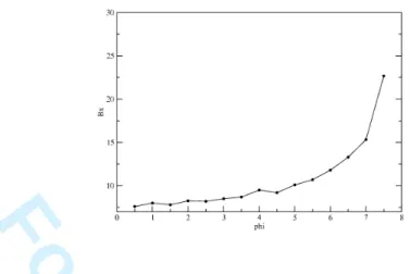
With the method developed in this paper, we have systematically looked at the effect of turning on the long range interaction, performing minimizations at regular φ increments. In Figure 5 we plot one of the coefficient of the exponent of the gaussian density (we have chosen Bx, but results
are independent of this choice) as a function of φ. We observe a highly non-linear dependence, indicating a compactification of the system even beyond the coil-globule transition. To observe a realistic coil-globule transition the long-range interaction itself should have a repulsive core and an attractive tail.
When looking at the details of the polymer configuration, proper quantities to measure are the end-to-end distance or the radius of gyration. At the present stage we measure the average density only. Other quantities are accessible with our formulation, but their theoretical treatment, though straight forward, is lengthy and will involve completely new numerical implementations. This is beyond the scope of this paper, where we want to establish the basic setting for the general formulation of confined polymer behavior in terms of a minimization principle and of mean field.
V. CONCLUDING REMARKS
The simplifying assumptions attend more directly to the physics, and these assumptions depend very much on the nature of the system to be studied. Taking these assumptions in order, we first
3 4 5 6 7 8 9 10 11 12 13 14 15 16 17 18 19 20 21 22 23 24 25 26 27 28 29 30 31 32 33 34 35 36 37 38 39 40 41 42 43 44 45 46 47 48 49 50 51 52 53 54 55 56 57 58 59 60
For Peer Review Only
FIG. 5: The coefficient Bx measured in terms of the strenght of the long-range attractive interaction φ.
For a Gaussian density like the one we have, a measure of Bxgives an idication of how peaked the density
distribution is. We observe a strong non-linear dependence, indicating a rapid compactification of the polymer as φ increases.
emebedded out system in a monomer grand ensemble. Since preprocessing assures that in practice one does not deal with the resulting extreme polydispersity, a fixed N ensemble is more relevant than fixed ζ. The corresponding inverse mapping has been attended to on numerous occasions (see e.g. [18]). The same formalism is indeed avaliable here (hinted at in eqs.(A15),(A16)).
Another restriction was to attractive long-range forces. We found however that the profile equation could indeed be pushed into the partially repulsive regime, although the validity of the minimum principle was in question; this is closely related to the functional Fourier transform for the repulsive component, likewise under uncertain control. An alternative approach lies in the use of the mean spherical model [19, 20] and its extensions. This is the aim of ongoing research.
Of course, there is the implicit assumption that pair forces suffice, whereas the action of pairs on singlets is a frequent important observation, leading e.g. to dihedral angle dependence in chains. Typically (see e.g. [21] for a very primitive example) one can simply create a multi-unit monomer to encompass only such forces, which then appear once more as pair forces.
Most blatantly, our approach has been restricted to homopolymers. Since the set of degrees of freedom of a monomer can include monomer type, this is no restriction at all if one is studying the effect on the full population of an assumed relative frequency of occurrence of next neightbors hetero-pairs. However, if we attribute a sense to the chain and the AB frequency differs from the BA frequency, the very convenient symmetry of the operator w is lost, and with it, the possibility
2 3 4 5 6 7 8 9 10 11 12 13 14 15 16 17 18 19 20 21 22 23 24 25 26 27 28 29 30 31 32 33 34 35 36 37 38 39 40 41 42 43 44 45 46 47 48 49 50 51 52 53 54 55 56 57 58 59 60
For Peer Review Only
e.g. of a specific long sequence of monomer types. The case of non-symmetric w has indeed been studied [22], but exercising the kind of control that we have in our current formulation remains a challenge.
Appendix A: Number Distribution
We first observe from (9) that if ˆN denotes the monomer number in a given configuration, than
N = h ˆN i =
Z
n(r)dr = h1|(ζ−1− w)−1ζ−1(ζ−1− w)−1|1i/Ξ(p) (A1)
= hζ1/2|(I − ζ1/2wζ1/2)−2|ζ1/2i/hζ1/2|(I − ζ1/2wζ1/2)−1|ζ1/2i (A2)
= 1/(1 − λ0) + O (1/(1 − λ1)) (A3)
where λ0 = λmax(ζ1/2wζ1/2) and λ1 is the next largest eigenvalue; λ1 < λ0 in a confined system.
If N is large, then
Ξ(p)(ζ) = hζ1/2|(I − ζ1/2wζ1/2)−1|ζ1/2i (A4)
is dominated by the “resonance” at λ0, so that if
(ζ1/2wζ1/2)ψλ0 = λ0ψλ0 (A5)
with normalized ψ, then
Ξ(p)[ζ] ∼ 1 1 − λ0
hψλ0|ζ
1/2|1i2 (A6)
There are now two consequences. On the one hand, we have
heiθ ˆNi = eiθζ0∂/∂ζ0Ξ(p)[ζ]/Ξ(p)[ζ] (A7)
= Ξ(p)[ζeiθ]/Ξ(p)[ζ] (A8)
∼
= (1 − λ0)/(1 − λ0eiθ) (A9)
so that the distribution of ˆN is given by
f (N ) = coef eiN θ(1 − λ0)/(1 − λ0eiθ) = λN0 (1 − λ0) (A10)
the very broad geometric distribution. It would appear that the N -ensemble must give a very poor representation of a given N . But on the other hand, we have from (5)
QN = ζ0−Nhζ1/2|(ζ1/2wζ1/2)N −1|ζ1/2i (A11) ∼ = ζ0−NλN −10 hψλ0|ζ 1/2i2, (A12) 3 4 5 6 7 8 9 10 11 12 13 14 15 16 17 18 19 20 21 22 23 24 25 26 27 28 29 30 31 32 33 34 35 36 37 38 39 40 41 42 43 44 45 46 47 48 49 50 51 52 53 54 55 56 57 58 59 60
For Peer Review Only
so that if FN is the canonical Helmholtz free energy,βFN − βΩ(p) = − ln QN + ln Ξ(p)[ζ] (A13)
∼
= N ln ζ0− (N − 1) ln λ0− ln(1 − λ0). (A14)
It follows that for any (N -independent) parameter variation
β(δFN − δΩ(p)) = µ 1 1 − λ0 −N − 1 λ0 ¶ δλ (A15)
which vanishes if ζ0 in (A5) is chosen so that
N = 1/(1 − λ0) (A16)
We conclude that for this choice of λ0, expectations at fixed N and in the monomer number
ensemble are in fact identical to leading order. This is not a surprise. Quite generally, for fluids, (see e.g [20]) inversion of the transformation from an N -ensemble to µ-ensemble follows the direct prescription above to leading order, with a correction term for expectations going as h(δN )2i/N2 . For fluids, this indeed goes as 1/N , but for a chain, using (19), as N0, and is therefore not a correction that vanishes as N → ∞. Another means of assessment is mandatory. In (12), we see that the relative correction to N has an amplitude ∼ (1 − λ0)/(1 − λ1); the same is true
for other expectations. Now suppose that, at some value of the system chemical potential µ, one has the pair λ0, λ1. Then if µ is increased by δµ, ζ(1/2)wζ(1/2) → exp(βδµ)ζ(1/2)wζ(1/2), so
that λ0 → exp(βδµ)λ0, λ1 → exp(βδµ)λ1. Then, as exp(βδµ)λ0 is made arbitrarily close to 1,
exp(βδµ)λ1 will never go beyond λ1/λ0, and the ratio (1 − λ0)/(1 − λ1) indeed goes as 1/N .
APPENDIX B: FLUCTUATIONS TO GAUSSIAN ORDER
We now take a first step towards including the effect of field fluctuations on the molecular density pattern. In this inital study, we have made one major approximation and several simplifying restrictions. The approximation is of course that of mean field, or selective neglect of fluctuations. On the assumption that fluctuations are Gaussian to leading order (examples in which this is not the case are far from rare, see e.g. [23]), a correction sequence is in primciple routine: we expand ln Ξ0 in (22) and (27) around ¯v of (29). Using δ2Ω0/δv(r)δv(r′) = δn0(r)/δv(r′)|v¯,
Ξ0[µ − 1 2φD− v] exp{− 1 2β v · φ −1v} = = exp ½ −β µ Ω0[µ − 1 2φD− ¯v] + 1 2¯v · φ −1v +¯ 1 2(v − ¯v) · ·δn 0 δv |¯v+ φ −1¸(v − ¯v) + . . .¶¾(B1) 2 3 4 5 6 7 8 9 10 11 12 13 14 15 16 17 18 19 20 21 22 23 24 25 26 27 28 29 30 31 32 33 34 35 36 37 38 39 40 41 42 43 44 45 46 47 48 49 50 51 52 53 54 55 56 57 58 59 60
For Peer Review Only
It readily follows (see e.g. [24]) that the density profile is given to the next order by simply averaging the density over the Gaussian field fluctuation:
n(r) = R n0[µ −12φD− ¯v − ∆]e −12 ³ ∆2 M −1(r,r) ´ d∆ R e− 1 2 ³ ∆2 M −1(r,r) ´ d∆ (B2) where M (r, r′) = φ−1(r, r′) − n′
0[µ −12φD− ¯v − ∆]; here, ∆ is the field amplitude fluctuation at r.
APPENDIX C: LIMIT OF TIGHT CONFINEMENT
We have seen, in Sec. II B, that in the absence of non-neighbor interactions, the large N monomer distribution is determined by the “resonance state” ψλ0 satisfying
(ζ1/2wζ1/2)ψλ0 = λ0ψλ0, (C1)
where λM AX = λ0 ∼ 1. Explicitely, since
hr|³ζ−1− w´−1|1i = hr|ζ1/2³I − ζ1/2wζ1/2´−1ζ1/2|1i
∼ 1
1 − λ0
hr|ζ1/2ψλ0ihψλ0|ζ
1/2|1i (C2)
we have under these circumstances, from (9)
n(r) ∼ 1 1 − λ0 ψλ0(r) 2, (C3) or since ψλ0(r) ∼ ψ1(r), n(r) ∼ ψ(r) 2 1 − λ0 = N ψ1(r)2 (C4)
In other words, increasing the chain length increases the mean density uniformly, as if the floppy chain is simply winding around more under the same confinement. This uninteresting behavior is refined by two interactions that have been ignored in getting (C4). First is the stiffness of successive pair orientations, equivalent to the monomers having coupled orientational degrees of freedom, a topic that has been addressed to some extent in this format in the past and will be attended to more forcefully in the future. Second is the effect of non-next neighbor interactions, which we have here studied in a preliminary fashion. The mean field v(r) that has been enountered will also have the effect of correlating pair orientations, and will of course alter the nature of the long chain resonant state. Let us see how this works. To keep the extrapolation from (C1-C4) transparent,
3 4 5 6 7 8 9 10 11 12 13 14 15 16 17 18 19 20 21 22 23 24 25 26 27 28 29 30 31 32 33 34 35 36 37 38 39 40 41 42 43 44 45 46 47 48 49 50 51 52 53 54 55 56 57 58 59 60
For Peer Review Only
let us rewrite (34) (using ζ = eβµ′) as,Ω1(ζ, φ) = Minv,ψ[
1 2v · φ
−1v − 2 lnh(ρe−βv)1/2|(ρ−1eβv)1/2ψi
+ lnh(ρ−1eβv)1/2ψ|I − (ρe−βv)1/2w(ρe−βv)1/2|(ρ−1eβv)1/2ψi]
= Minv, ¯ψ
· 1
2v · φ−1− 2 lnh(ρe−bv)1/2| ¯ψi + lnh ¯ψ|I − (ρe−bv)1/2w(ρe−βv)1/2| ¯ψi
¸
(C5)
Hence, according to (38), ¯ψ = (ζ−1eβv)1/2ψ is normalized, h ¯ψ| ¯ψi = 1 and from (39),
n = N ¯ψ2 (C6)
Near resonance is now signaled by the approximate validity of
³
I − (ζe−βv)1/2w(ζe−βv)1/2´ψ = ¯¯ λ ¯ψ (C7)
with small ¯λ > 0. Eq. (50) then tells us at once that using the exact
φ−1v = −n, (C8)
we have
N = 1/¯λ (C9)
There are two ways of making use of the approximation C7. Most directly, we substitute (C6-C9) into (C5), obtaining
βΩ1 ∼ Minn
·1
2n · φn − 2 lnh(ζe
βφn)1/2|n1/2i¸ (C10)
This is obviously too sweeping an approximation: by using what is effectively a first order correction in the argument of a variational principle, the role of the next-neighbor w in βΩ1 has vanished.
But we can pick up the next order by working instead at the “profile equation” level. It is only necessary to substitute (C6, C8, C9) directly into (C7) to rewrite the latter as
(ζeβv)1/2w(ζe−βv)1/2n1/2= µ 1 − 1 N ¶ n1/2, (C11) and hence as e−β2(u−φn)weβ2(u−φn)n1/2 = µ1 − 1 N ¶ e−βµ′0n1/2 ≡ Λn1/2 (C12) (µ′
0 is the global chemical potential). The operator in (C12) has a positive kernel, hence by
Jentchke’s extension of Perron-Frobenius [25], the positive eigenfunction is unique (up to a mul-tiplicative constant) and Λ is real and maximal. This leads to what is in principle a simple
2 3 4 5 6 7 8 9 10 11 12 13 14 15 16 17 18 19 20 21 22 23 24 25 26 27 28 29 30 31 32 33 34 35 36 37 38 39 40 41 42 43 44 45 46 47 48 49 50 51 52 53 54 55 56 57 58 59 60
For Peer Review Only
numerical iteration: start eg. with φ = 0, compute the eigenfunction n1/2 and normalize it to get
R
n(r)dr = N . At the kth stage of the M-fold iteration, replace φ by (k/M )φ and repeat the
pro-cess using the current function n. An alternative strategy is to parameterize n and determine the parameters by Galerkin, i.e. integrate (C12) with weight function and solve the resulting algebraic equation.
APPENDIX D: DETAILS ON NUMERICS
From preliminary simulation studies we had noticed how in the absence of a repulsive core interaction between monomers we could not converge to a stationary density. Instead the density, and therefore the total particle number, either kept on growing or shrank to zero, depending on the value of the external chemical potential. This numerical instability occures as a result of the closeness to the resonance. In these simulations we noticed, on the other hand, that despite the fact that the density itself kept changing, the global shape of density profile reached a steady state. We therefore decided to study the normalized density p(r) = n(r)/N . Once we had formulated the problem consistently in terms of p all the numerical instabilites desappeared and we were able to determine the corresponding stady state densities and total particle numbers. The minimization is done using a Metropolis Monte Carlo algorithm at fixed temperature, starting from a suitable ansatz for the functional form of p(r). This is one of many possible techniques, and is not optimized in any well-defined sense. We can freely impose the form of the next neighbor potential, and therefore w(r, r′), the external confining potential u(r), and the long range interaction φ(r, r′). The
main numerical difficulty arises from the need of evaluating a functional involving 6-dimensional integrals nesting 3-dimensional integrals, such as
Z q p(r)eβ2(µ′(r)+N R φ(r,r′′)p(r′′)dr′′ )w(r, r′)eβ2(µ′(r′)+NRφ(r′,r′′)p(r′′)dr′′)q p(r′)dr dr′ (D1)
It turns out it is prohibitive to try to evaluate these terms directly by the use of a simple grid. Already when using 10 discretization points simulations are too slow, while the precision is very poor. To achieve higher accuracy in the integration, we use a Legendre-Gauss quadrature method with either 6 or 8 points in each linear direction.
As a test system we have chosen a square well external potential with µ = −µ0 inside; a
harmonic n.n. potential, leading to w(r, r′) = exp(−C
h(|r − r′| − ρ1)2); a long-range step potential
φ = ClrΘ(x − ρ2), where µ0, Ch, Clrare energy constants, and ρ1 and ρ2are characteristic lengths.
In the following we take the system size to be L = 1, Ch = 5, and ρ1 = 0.2. As ansatz for the
3 4 5 6 7 8 9 10 11 12 13 14 15 16 17 18 19 20 21 22 23 24 25 26 27 28 29 30 31 32 33 34 35 36 37 38 39 40 41 42 43 44 45 46 47 48 49 50 51 52 53 54 55 56 57 58 59 60
For Peer Review Only
probability density we take the composition of three Gaussian in the three spatial directions, for a total of 6 parameters: Bx,By,Bz,X0,Y0 and Z0.
p(x, y, z) = A e−Bx(x−X0)2e−By(y−Y0)2e−Bz(z−Z0)2 (D2)
At each iteration of the algorithm the normalization of n is verified so thatR
p(x, y, z)dx dy dz = 1, and the value of A is changed accordingly.
[1] R.J. Ellis, Curr. Opin. Struct. Biol11:114-119 (2001)
[2] D. Thirumalai, D.K. Klimov, G.H. Lorimer, PNAS 100:11195-11197 (2003) [3] D.K. Eggers, J.S. Valentine, J. Mol. Biol. 314:911-922 (2001)
[4] P.G. de Gennes, “Scaling concepts in polymer physics”, Cornell University Press (1979) [5] I.M. Lifshits, Sov. Phys. JETP 55, 2408 (1968)
[6] S. Pasquali and J.K. Percus, J. Chem. Phys. 125, 064906 (2006) [7] H.L. Frisch and J.K. Percus, J. Phys. Chem. B 105, 11834 (2001) [8] J.K. Percus, J. Stat. Phys. 106, 357 (2002)
[9] B. Widom, J. Chem. Phys. 39, 2808 (1963)
[10] M. Kac, in “Applied Probability”, ed C.A. MacColl, McGraw Hill, NY (1957) [11] A.J.F. Siegert, Physica (supp.) 26, 530 (1960)
[12] J. Hubbard, Phys. Rev. Lett. 3, 11 (1959)
[13] R.L. Stratonovich, Sov. Phys. Doklady 2, 416 (1958)
[14] G. Giacomin, “Random Polymer Models”, World Scientific (2007) [15] P. Flory, “Statistical mechanics of chain molecules”, Wiley (1969) [16] M. Huggins, J. Phys. Chem. 46, 151 (1942)
[17] D. Poland, H.A. Sheraga, “Theory of Helix-Coil Transitions in Biopolymers”, Academic Press, New York (1970)
[18] J.L. Lebowitz, J.K. Percus, and L. Verlet, Phys. Rev. 153, 2506 (1967) [19] J.K. Percus and G.J. Yevick, Phys. Rev. 136, 290 (1964)
[20] J.L. Lebowitz and J.K. Percus, Phys. Rev. 144, 251 (1966)
[21] K.K. Muller-Nedebock, H.L. Frisch and J.K. Percus, Phys. Rev. E 67, 011801 (2003) [22] H.L. Frisch and J.K. Percus, Phys. Rev. E 64, 011805 (2001)
[23] R. Rajaraman, Phys. Rep. C 21, 227 (1975) [24] J.K. Percus, Physica A 172, 1 (1991) [25] R. Jentzsch, Crelles Jour. 141, 235 (1912)
2 3 4 5 6 7 8 9 10 11 12 13 14 15 16 17 18 19 20 21 22 23 24 25 26 27 28 29 30 31 32 33 34 35 36 37 38 39 40 41 42 43 44 45 46 47 48 49 50 51 52 53 54 55 56 57 58 59 60