Air
Quality
Value Theory:
Ozone
E
Applications of Extreme
Return Levels of Extreme
vents in
Chicago and
Surrounding Areas
by
Elizabeth Ndayu Rider
Submitted to the Department of Earth, Atmospheric
and Planetary Sciences in Partial Fulfillment of the
Requirements for the Degree of Bachelor of Science
in Earth, Atmospheric, and Planetary Sciences at the
Massachusetts Institute of Technology
May 16, 2017
Copyright 2017 Elizabeth Ndayu Rider.
All rights reserved.
The author hereby grants to MIT permission to reproduce and to distribute publicly paper and electronic copies of this thesis document in whole or in
part in any medium now known or hereafter created.
Author ...
Signature redacted
Departmentf Earth, Atmospheric, a d
lanetary
SciencesCertfie by
SN
May 16, 2017Certified by ...
Sinaur r edacted
...
Accepted by
/1
Professor Noelle Eckley Selin
Thesis Supervisor
.Signature
redacted...
Richard P. Binzel Chair, Committee on Undergraduate Program
MASSACHUS
IT
ITUTE
OF TECHNOLOGY
SEP 28
2017
LIBRARIES
Contents
List of Figures 3
List of Tables 4
1 Introduction 6
1.1 A Review of Ozone Chemistry. . . . .
6
1.1.1 CO Oxidation mechanism . . . . 7
1.1.2 Methane oxidation mechanism . . . . 8
1.2 Regulation of Tropospheric Ozone . . . . 10
1.3 Extreme Value Theory . . . . 11
2 Methods 13 2.1 D ata . . . . 13
2.2 Extreme Value Theory . . . . 14
2.2.1 Generalized Pareto Distribution . . . . 15
2.2.2 Return Level Estimation . . . . ... . . . . 15
3 Results 15 4 Discussion 19 5 Conclusion 20 6 Acknowledgments 21 7 Site By Site Analyses 25 7.1 U rban Sites . . . . 25
7.1.1 3300 E. CHELTENHAM PL. . . . . 25
7.1.2 6545 W. HURLBUT ST. . . . . 27
7.1.3 5720 S. ELLIS AVE. . . . . 27
7.1.4 665 DUNDEE RD. . . . . 28
7.1.5 HURLBURT & MACARTHUR . . . . 28
7.1.6 508 E. GLEN AVE. . . . . 29 7.2 Suburban/Rural Sites . . . . 30 7.2.1 729 HOUSTON . . . . 30 7.2.2 750 DUNDEE ROAD . . . . 32 7.2.3 531 E. LINCOLN . . . . 32 7.2.4 1820
S.
51ST AVE. . . . . 33 7.2.5 4500 W. 123RD ST. . . . . 33 7.2.6 RT. 53 ... ... 347.2.7 LIBERTY ST.
&
COUNTY RD. . . . . 347.2.8 FIRST ST. & THREE OAKS RD. . . . . 35
7.2.9 2200 N. 22ND . . . . 35
7.2.10 HEATON & DUBOIS . . . . 36
7.2.12 200 W. DIVISION ... 37
7.2.13 54 N. WALCOTT ... 37
7.2.14 HICKORY GROVE & FALLVIEW ... 38
7.2.15 13TH & TUDOR ... 38
7.2.16 1405 MAPLE AVE . ... 39
List of Figures
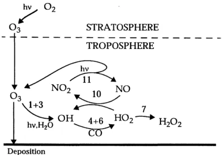
1 Chemical formation of ozone in the troposphere. Tropospheric ozone is produced when hydrocarbons and volatile organic com-pounds are oxidized by the hydroxyl radical OH in the presence of reactive nitrogen oxides (NO,) (Jacob 1999 ). . . . . 6
2 (Jacob 1999, adapted from Sillman et al., 1990. . . . . 9 3 Probability of ozone extremes as a function of temperature.
Ozone concentrations are dependent on temperature, partic-ularly in the Northeast United States, while in the Southeast United States, ozone concentrations depend more heavily on relative humidity. (Jacob and Winner (2009) [1], adapted from Lin et al. (2001) [2]). . . . . 10
4 National trend of urban ozone concentrations. Based upon ob-servations from 111 locations in urban areas, ozone concen-trations have been decreasing over the period spanning from 2000 to 2015. When adjusted for weather, the overall change
between 2000 and 2015 levels are less pronounced [3] . . . . 11 5 Left: JJA Ozone Concentrations for an example site for 1992.
Right: JJA Ozone Concentrations for an example site from
1992 to 2013. ... ... 12
6 Map of AQS sites used in this study. Red circles are subur-ban/rural sites, while green circles lie in Chicago, Peoria and
E lgin . . . . 13
7 Range of compiled ozone concentrations for Period 1 [1992-2002] in rural and urban areas. Ozone concentrations in rural
areas exceed those in urban areas. . . . . 18 8 Range of compiled ozone concentrations for Period 2
[1992-2002] in rural and urban areas. Both rural and urban areas saw decreases in extreme ozone concentrations, and an increase in the average. . . . . 18 9 Time series for an example urban site (3300 E. CHELTENHAM
PL.) displaying JJA DM8A 03 concentrations from 1990 to 2013. 25
10 Changes in the return level of ozone concentrations for Period 1 (left) and Period 2 (right) for an example urban site (3300 E.
CHELTENHAM PL.). . . . . 25
11 Density distribution of ozone concentrations at an example ur-ban site (3300 E. CHELTENHAM PL.). . . . . 26
12 Time series for an example suburban/rural site (729
HOUS-TON) displaying JJA DM8A 03 concentrations from 1990 to
2013... ... 30
13 Changes in the return level of ozone concentrations for Period
1 (left) and Period 2 (right) for an example suburban/rural site
(729 HOUSTON). . . . . 30
14 Density distribution of ozone concentrations at an example sub-urban/rural site (729 HOUSTON). . . . . 31
List of Tables
1 Table of site locations. . . . . 2 Site by Site averages of ozone concentrations. For the
pur-poses of this study, sites in Chicago are considered urban, while other sites in Cook County are considered suburban. The site in Bondville, IL refers to a rural site from CASTNet, calculated
by Phalitnokiat et al., (2016). . . . . 3 Results of site by site 20-year return level analysis for Period
1 (1992-2002) and Period 2 (2003-2013). All sites' 20-year
re-turn levels decreased between Period 1 and Period 2. Sites in Chicago and Cook County experienced similar magnitudes of change, though the site in Bondville, IL (from Phalitnonkiat, et al., (2016)) experienced the largest decrease of
4 3300 E. CHELTENHAM PL. . . . .
5 6545 W. HURLBUT ST. . . . .
6 5720 S. ELLIS AVE. . . . .
7 665 DUNDEE RD. . . . .
8 HURLBURT & MACARTHUR . . . .
9 508 E. GLEN AVE. . . . . 10 729 HOUSTON . . . . 11 750 DUNDEE ROAD . . . . 12 531 E. LINCOLN . . . . 13 1820
S.
51ST AVE. . . . . 14 4500 W. 123RD ST. . . . . 15 RT . 53 . . . .16 LIBERTY ST. & COUNTY RD. . . . .
17 FIRST ST. & THREE OAKS RD. . . . .
18 2200 N. 22ND . . . .
19 HEATON & DUBOIS . . . .
20 409 MAIN ST. . . . . 21 200 W. DIVISION . . . . 22 54 N. WALCOTT . . . . 23 HICKORY GROVE & FALLVIEW . . . . 24 13TH & TUDOR . . . .
25 1405 MAPLE AVE . ...
all Illinois sites. 14 16 17 26 27 27 28 28 29 31 32 32 33 33 34 34 35 35 36 36 37 37 38 38 39
Air Quality Applications of Extreme Value Theory: Return Levels of Extreme Ozone Events in Chicago and Surrounding Areas
By
Elizabeth Ndayu Rider
Submitted to the Department of Earth, Atmospheric and Planetary Sciences in Partial Fulfillment of the Requirements for the Degree of Bachelor of Science in Earth, Atmospheric, and Planetary Sciences at the Massachusetts
Institute of Technology
Abstract
To quantify the effects of the NO, SIP call in urban and rural locales, surface ozone data from the Air Quality System is analyzed. Methods from extreme value theory are applied to calculate and compare 20-year return levels at 5
urban and 17 rural/suburban sites in Illinois based upon maximum daily 8-. hour average ozone concentrations from summer (JJA) for two periods (1992-2002 and 2003-2013) and a threshold of 70 (ppb). Between the two periods, 21 out of 22 sites experienced a decrease in 20-year return levels. The magnitude of these decreases does not indicate a strong correlation between population density and air quality improvements, however, further analysis is required.
1
Introduction
Tropospheric ozone is hazardous to human and environmental health. Ozone has been shown to have damaging effects on crop production with economic reper-cussions [4]. Reduced crop yields from ozone have important reperreper-cussions on food security under a changing climate [5]. Attempts at quantifying the annual agricultural costs of tropospheric ozone ranged from $11-18 billion (USD2000)
[6] to $14-26 billion (USD2000) [7] based upon 2000 emissions. Ozone can affect
human respiration and damage lung tissues [8, 9], and is associated with an increased risk of death from respiratory causes [10]. Fann and Risley (2013) [11] found that ozone reductions between 2000 and 2007 in the United States were associated with 880-4100 avoided premature mortalities. Anenberg et al, (2010) [12] estimated that globally, anthropogenic ozone was associated with 0.7
+/-0.3 million respiratory mortalities annually or 6.3 +/- 3.0 million years of life
lost.
hv
02
03
STRATOSPHERE
TROPOSPHERE
hv
03
NO
210NO
1+3
7
hvH
20
OH
4+6
HO
2H
20
2Deposition
Figure 1: Chemical formation of ozone in the troposphere. Tropospheric ozone is produced when hydrocarbons and volatile organic compounds are oxidized
by the hydroxyl radical OH in the presence of reactive nitrogen oxides (NO,)
(Jacob 1999 ).
1.1
A Review of Ozone Chemistry
Tropospheric ozone is produced via photochemical oxidation of carbon monoxide
by the hydroxyl radical (OH) in the presence of reactive nitrogen oxides (NO, =
NO + NO2). The primary sink of tropospheric ozone is photolysis in the pres-ence of water vapor, however, dry deposition is also an important sink beneath the continental boundary layer (~- 2 km). Ozone's lifetime in the troposphere ranges from a few days to weeks and ozone concentrations tend to be highest in the summertime [1].
The chemical coupling of 03, HO,, and NO, is represented in Fig. 1. While
some 03 is a result of transport from the stratosphere, the primary sources of tropospheric ozone are due to chemical production within the troposphere. These reactions are discussed in more detail below; reaction numbers are chosen to match reactions depicted in Fig. 1 from Jacob, (1999).
To start, 03 is photolyzed to form OH radicals by the following reactions
03 +
hv-02 + O(D)
(1)O(D)+ M - O+ M (2)
O(QD)
+
H20
- 2OH (3)OH is produced when 03 is photolyzed by photons with wavelength
be-tween 300 and 320 nim. Reaction 3 will proceed readily when H20 is readily
available (e.g. lower troposphere). OH is a highly reactive compound that rapidly oxidizes CO, CH4, and NMVOCs. These reactions are summarized
be-low.
1.1.1 CO Oxidation mechanism
Sources of CO in the troposphere include oxidation of methane and other hy-drocarbons, biomass burning, fossil fuel combustion/industry, vegetation and oceans. Sinks include tropospheric oxidation by OH, soil uptake and transport to the stratosphere. Most of the CO in the current troposphere is anthropogenic.
CO will form 03 in the troposphere when it is oxidized by OH. The oxidation of CO proceeds by
CO
+
OH- C02+H
(4)H+02+M - H02 + M (6)
HO2 is depleted when HO2 self-reacts to form hydrogen peroxide by the
following reaction:
H02
+
H02 - H202 + 02 (7)Otherwise, H02 can react with NO to form N02 which will then produce ozone when photolyzed:
NO2 + hv -+ NO+ 03
for a net reaction of
net: CO + 202 - C02 + 03
The CO oxidation mechanism of 03 production is initiated by the source of HO, (HO, = H + OH + HO2) from Reaction 3. When HO, is depleted through
Reaction 7, the mechanism is terminated. The overall efficiency is determined
by NOT.
1.1.2 Methane oxidation mechanism
Methane has both natural and anthropogenic sources. Methane occurs natu-rally from wetlands, termites and other sources, while its anthropogenic sources include livestock, rice paddies, and natural gas. Methane is removed from the troposphere after being oxidized by OH, deposited in soils, or transported to the stratosphere.
-The mechanism by which methane is oxidized to form 03 is dependent on the concentration of NO,. That is, in a high NO, regime the net reaction by which CH4 is oxidized is:
CH4 +10 02 -+ C02+H2
0+50
3+20HIn this reaction, one molecule of methane produces 5 molecules of 03 and
OH radicals.
In a NOT-limited regime, the net reaction of CH4 oxidation is
CH4
+ 30H
+202
-+ CO2+3
H20
+ HO2where no ozone is produced, and OH is consumed.
This methane oxidation mechanism is similar to that of other hydrocar-bons, however, other hydrocarbons have smaller global sources. Their specific reactions are omitted (see [13]).
The NOT, VOC, and CO precursors of 03 have anthropogenic sources
including fuel combustion and biomass burning, as well as natural sources in-cluding lightning, wildfires, soils, and vegetation. In polluted regions such as the eastern United States, anthropogenic emissions of NO., VOC, and CO lead to high-03 episodes endangering public health.
Ozone is dependent on NO. and VOCs in two regimes. In the NO.-sensitive regime where there concentrations of NO, are low, and concentrations of VOCs are high, 03 and NO, have a direct relationship, in which, 03 concen-trations increase with increasing NOT, and stay the same with increasing VOC concentrations. Meanwhile, in the NO-saturated or VOC-sensitive regime, concentrations of 03 increase with increasing VOC concentrations, while 03
concentrations decrease with increasing NO.. In Fig. 2, the thick black line delineates the regime between NO_-limited and NO1-saturated regimes. To the upper left is the NO-limited regime, where NO increases result in increased
U
160
200
E5
-180
0160
-4
4140 034 3 - 40120 120 100 100 2 - 8080
60
60 4020
0
2 4 6 8 10 12 14 16 18NOX emissions, 1011 molecules Cm-
2 s-IFigure 2: (Jacob 1999, adapted from Sillman et al., 1990.
ozone concentrations. To the right is the NO-saturated regime, where 03 concentrations decrease with increasing NO, and increase with increasing hy-drocarbons. This system of ozone and its precursors is nonlinear; defining and characterizing these regimes can be difficult but important for creating effective environmental policy. In the NO-saturated regime, a decrease in NO, due to NO, emission controls can cause an increase in 03 concentrations. There is also evidence that rural and urban areas are controlled by their differing regimes- (e.g. [14]). In rural ares, ozone production is NO,-limited, and almost independent of hydrocarbon concentrations. In urban air, in contrast, ozone concentrations depend on both NO, and hydrocarbon concentrations. In this way, concentrations of ozone are often higher in rural areas than in urban areas (e.g. [15]). Because ozone chemistry is a complex, non-linear system, attempts to control 03 concentrations by limiting emissions of precursors can have unin-tuitive effects.
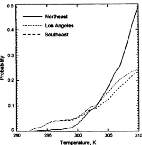
Ozone concentrations have been shown to be dependent upon tempera-ture, with higher temperatures increasing the probability of ozone exceedances (Fig. 3) especially in the Northeastern United States [1]. Other meteorologi-cal variables (e.g. biogenic emissions of hydrocarbons, atmospheric circulation, photochemical environment, relative humidity, cyclone frequency, among oth-ers) have all been found to affect ozone concentration as well (e.g. [16]).
05 -4 --.. Southeast 03 2 0 290 295 300 305 310 Temperature, K
Figure 3: Probability of ozone extremes as a function of temperature. Ozone concentrations are dependent on temperature, particularly in the Northeast United States, while in the Southeast United States, ozone concentrations depend more heavily on relative humidity. (Jacob and Winner (2009) [1],
adapted from Lin et al. (2001) [2]).
1.2
Regulation of Tropospheric Ozone
The US EPA has regulated ozone as a criteria air pollutant since 1971 after the Clean Air Act [17] was passed. The standard for ozone has decreased from 80
ppb averaged over 1 hour (not to be exceeded more than once a year) in 1971,
to 70 ppb averaged over 8 hours (annual fourth-highest daily maximum 8 hour average concentration, averaged over 3 years) in 2015. In 1997, the EPA revised the 1-hour ozone standard to replace it with an 8-hour standard that used the annual fourth-highest DMA8 to be mroe protective.
In 2015, approximately 127 million people lived in 241 counties that ex-ceeded the revised national ground-level ozone standards (75 ppb) which has since been decreased to its current level of 70 ppb [18]. Fig. 4 shows the na-tional trend in urban ozone concentrations, highlighting that with decreasing standards for ozone, concentrations of ozone have decreased as well.
Background levels of ozone are dependent on season, altitude and total
03 concentrations. Estimates of background 03 vary between 15-35 ppb while
natural levels are estimated to be 10-25 ppb, not exceeding 40 ppb [19]. Un-der a changing climate, background levels 03 are uncertain. Some estimates indicate that background levels of surface 03 will increase due to increases in photochemistry from higher temperatures [20], while other studies cite increased water vapor as a factor that could reduce ozone concentrations [1]. Still other studies indicate that changes in background ozone levels will be regionally de-pendent [21]. Beyond climate, it is predicted that background ozone levels in the
US will increase due to the increasing importance of Intercontinental transport
Northeast
of ozone and its precursors from East Asia [22, 20].
The health costs due to global ozone pollution are estimated to reach $580 billion (USD2000) by 2050, with mortalities from acute exposure exceeding 2 million [23). The agricultural costs are expected to increase with with estimates of future global agricultural losses worth $12-35 billion (USD2000) in the year
2030 [6]. At special risk to ozone exposure are those with preexisting respiratory
and cardiovascular conditions, infants and those in their old-age, low-income populations with poor access to quality healthcare, and those living in urban areas who are exposed to higher concentrations of ozone daily. The racial and socioeconomic disparities in the United States, where low-income and minority communities are exposed to higher concentrations with fewer health resources makes air quality an issue of environmental justice (e.g. [24, 25, 26, 27]).
National Urban Ozone Trend (111 Locations)
~55
--45
Adjustec for Weather
40 - - Unadjsted for Weather
0 00 C D0 0 0 c0 0 CD 0 0D 0 0 C0 0 ,
Figure 4: National trend of urban ozone concentrations. Based upon obser-vations from 111 locations in urban areas, ozone concentrations have been decreasing over the period spanning from 2000 to 2015. When adjusted for weather, the overall change between 2000 and 2015 levels are less pronounced
[3].
Significant reductions in ozone concentrations occurred in the mid-2000s following stricter federal emissions standards on vehicles, and due to require-ments of the federal NO, State Implementation (SIP) Call [28].
1.3
Extreme Value Theory
Extreme value theory (EVT) provides a statistical methodology to better un-derstand extreme events [29). Specifically, EVT allows the tails of distributions to be examined. In the case of 03, tails are often long or heavy (skewed right). Because of these infrequent high 03 days, the distribution is non-Gaussian, and must be fitted before analysis. In this paper, with the threshold set to 70 ppb, the ozone NAAQS exceedances are analyzed. Return levels are calculated to describe the probability of exceeding this threshold (see Section 2.2.2), and are thus used as a method to quantify the effectiveness of the NO, SIP call.
Previous studies have applied extreme value theory to high ozone pollution events in the United States.. Rieder et al., (2013) quantified the 1-year and 5-year return levels as well as the expected frequency of ozone NAAQS exceedances in the eastern United States using 23 sites from the Clean Air Status and Trends Network (CASTNet). Their study used data from two periods, 1988-1998 and
1999-2009, each fit to the Generalized Pareto Distribution (GPD). Their results
confirmed declines in frequency and magnitude of high ozone pollution events following emission controls. Additionally, their results indicate that the NO,
SIP Call, among other emissions reductions, had a large effect on return levels,
as the 5-year return levels of the period 1999-2009 were roughly equivalent to the 1-year return levels of the earlier time period (1988-1998). They found the strongest drop in return levels was about 13 ppb observed in the Northeast, with the Mid-Atlantic and Great Lakes regions each experiencing an 8 ppb drop in return levels.
Expanding upon the work of Rieder et al,. (2013), Phalitnonkiat et al.,
(2016) quanitified the 20-year return levels for 25 CASTNet sites, using the GPD. Their study focused on two periods, 1992-2002 and 2003-2013, to
inves-tigate the effects of the NO. SIP call on extreme ozone events. Their results indicate that, following the NO. SIP call, the tails of ozone distributions be-came heavier at most sites. Their study also improved methodologies, as they compared the benefits of the Hill estimator with those of the Maximum Likeli-hood Estimator (MLE) using synthetic data. Their results indicate that under certain conditions, the MLE is likely to understimate the tail of the distribution. This thesis will center around these NO, reductions in Chicago and sur-rounding areas using the Air Quality System. While other studies [30, 31, 32] have studied return levels of extreme ozone events in the United States, these studies relied upon rural data from the Clean Air Status and Trends Network (CASTNet). As the methods put forth in Extreme Value Theory rely on heavy-tailed distributions, this paper will address the following questions: how did the
NO, SIPs affect the frequency of extreme ozone events in the city of Chicago
when compared to surrounding rural areas? Can the same EVT methods used previously for rural areas be used in this analysis? Are the values generated for return levels and probability useful for evaluating policy in urban areas?
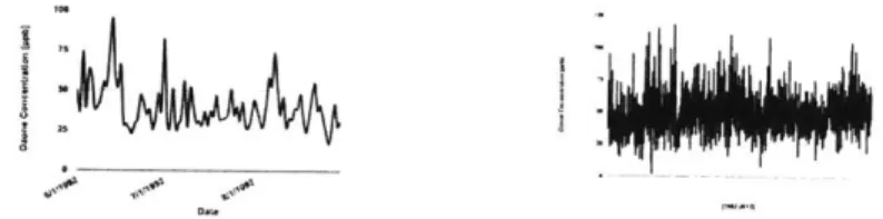
Figure 5: Left: JJA Ozone Concentrations for an example site for 1992. Right: JJA Ozone Concentrations for an example site from 1992 to 2013.
2
Methods
2.1
Data
Daily maximum eight hour concentrations from the EPA Air Quality System
(AQS) are used. The AQS is a database of monitored ambient air quality data
compiled by the EPA. Unlike other networks, (e.g. CASTNet, which has 95 sites based in rural locations), the sites within the AQS is more expansive, covering various location settings. Because of the great number of sites and the sites, diversity of locations, the AQS can be used to compare and contrast air quality in rural, urban, and suburban areas. The EPA's calculated DM8A
03
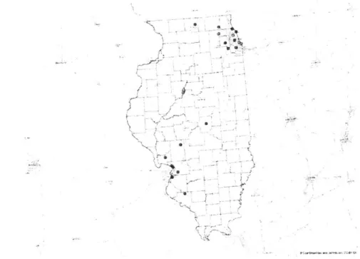
were used. Only days with with full 24 hour coverage are included and only sites with at least 90% completion over the whole period (1992-2013 summertime(JJA)) were considered. From IL, 22 sites fit these criteria, 6 of which lay in
the following cities Chicago, Peoria, and Elgin. The addresses and coordinates of each site are listed in Table 1 and mapped in Fig. 6. An example time series is displayed in Fig. 5, for a single year (1992), and for the span of all years (1992-2013). Note that the time series of 03 concentrations (Fig. 5) are highly variable and auto-correlated, reflecting the close coupling of atmospheric chemistry and local meteorology.
Figure 6: Mlap of AQS sites used in this study. Red circles are suburban/rural sites, while green circles
lie
in Chicago, Peoria and Elgin.List of Sites
Address City County Latitude Longitude
3300 E. Chel- Chicago Cook 41.76 -87.55
tenham Pl.
5720 S. Ellis Ave. Chicago Cook 41.79 -87.60
6545 W. Hurlbut Chicago Cook 41.98 -87.79
St.
665 Dundee Rd. Elgin Kane 42.05 -88.27
Hurlburt & Peoria Peoria 40.69 -89.61
MacArthur
508 E. Glen Ave. Peoria Heights Peoria 40.75 -89.59
1820 S. 51st St. Cicero Cook 41.86 -87.75
4500 W. 123rd St. Alsip Cook 41.67 -87.73
531 E. Lincoln Evanston Cook 42.06 -87.68
729 Houston Lemon Cook 41.67 -87.99
750 Dundee Rd. Northbrook Cook 42.05 -88.27
Rt. 53 Lisle DuPage 41.81 -88.07
Liberty St. & Jerseyville Jersey 39.11 -90.32
County Rd.
First St. & Three Cary McHenry 42.22 -88.24
Oaks
Rd.2200 N. 22nd Decatur Macon 39.87 -90.32
Heaton & Dubois Nilwood Macoupin 39.40 -89.81
409 Main St. Alton Madison 38.89 -90.15
200 W. Division Maryville Madison 38.73 -89.96
54 N. Walcott Wood River Madison 38.86 -90.11
Hickory Grove & N/A Randolph 38.18 -89.79
Fallview
13th & Tudor East Saint Louis Saint Clair 38.61 -90.16
1405 Maple Ave. Loves Park Winnebago 42.33 -89.04 Table 1: Table of site locations.
As in Phalitnonkiat et al., (2016) [31], the data are divided into 2 periods
(1992-2002 and 2003-2013) to assess the impact of the NO, SIP call on ozone
extremes.
2.2
Extreme Value Theory
Rieder et al., (2013) [30] applied the methods from Extreme Value Theory to fit a Generalized Pareto Distribution (GPD) to the heavy tails of MDA8 03, allowing the calculation of return levels for high 03 pollution events. The GPD is a versatile model that can fit the different shapes of distributional tails using shape
and scale parameters (Coles, 2001). As in Rieder et al., (2013) [301 the Maximum Likelihood Estimator (MLE) is used to calculate a shape parameter. These calculations are performed using the Peaks Over a Threshold model (POT) and the POT-Package for R [33, 34].
2.2.1 Generalized Pareto Distribution
In order to estimate return levels, the data are fitted to a Generalized Pareto Distribution (GPD). The GPD is better adapted to the heavy tails of high ozone events and is defined as,
H(x) = 1 - (1+( (5)
where x are the MDA8 of 03, u is the threshold, and a > 0 is the scale
parameter, and C is the shape parameter [33]. To match the current EPA standard for ozone, the threshold u = 70 ppb. The size and shape parameter are estimated using the Maxmimum Likelihood Estimator (MLE) as in [30, 32].
2.2.2 Return Level Estimation
The return levels for RT years is then given by
R)T = H(x)- (1 -)
(6)
and describes the probability of x exceeding the threshold u in designated time period T. Here, T is set to 20 years and u is set to 70 ppb, the current EPA standard for ozone in the United States.
3
Results
Listed in Table 2 are the averages and standard deviations for each site during both periods. These sites are broken down into two categories: Urban and Suburban/Rural. Based upon these initial calculations of means and standard deviations between Period 1 (1992-2002) and Period 2 (2003-2013), there is little change following the NO, SIP call, although there is a change in 20-year return levels as described below. Many sites have averages that increase slightly between periods, but these changes are of such small magnitude that they are likely not statistically significant, especially given the natural variability of ozone chemistry (Fig. 5). The largest change in means between Period 1 and 2 comes from a site in Bondville, IL as calculated by Phalitnonkiat et al., (2016).
Of the 22 sites in Illinois, 21 sites experienced decreases in their 20-year
return level (Table 3). The highest 20-year return levels calculated for Period 1 was 101.9 ppb at 1820
S.
51st St. in Cicero and 6545 Hurlbut St. in Chicago (both in Cook County), and the lowest 20-year return level for the same period was 82.3 ppb at Hurlburt & Macarthur in Peoria, IL. For Period 2, the highest 20-year return level was 98.6 ppb at 750 Dundee Rd. in Northbrook and thelowest was 78.6 ppb at 1405 Maple Ave. in Loves Park. The largest change was a decrease of 11.2 ppb at 2200 N 22nd in Decatur, and the smallest change was a decrease of 0.482 ppb at 531 E. Lincoln in Evanston. The 20-year return level for one site, 13th and Tudor in East Saint Louis, increased by 2.49 ppb between the two periods. Also listed in Table 3 are the 20-year return levels calculated
by Phalitnonkiat et al., for a site in Bondville, IL. The change in 20-year return
levels for this site exceeds those from the AQS.
AVERAGE OZONE CONCENTRATIONS BY SITE AND PERIOD
[ppb]
SITE ADDRESS PERIOD 1 PERIOD 2
MEAN (SD) MEAN (SD)
3300 E. Cheltenham Pl. 49.7 (16.8) 49.5 (13.3)
5720
S.
Ellis Ave. 44.2 (16.2) 44.5 (13.9)6545 W. Hurlbut St. 42.9 (16.3) 46.6 (13.4)
665 Dundee Rd. 48.0 (15.1) 46.5 (13.0)
Hurlburt & MacArthur 47.0 (13.0) 44.1 (11.3)
508 E. Glen Ave. 50.3 (13.5) 48.9 (11.7)
Urban 46.9 (15.6) 46.7 (12.9)
Rt. 53 43.8 (14.4) 43.2 (12.9)
Liberty St. & County 54.6 (15.0) 50.6 (13.7) Rd.
First St. & Three Oaks 49.8 (15.4) 45.7 (12.8)
Rd.
2200 N. 22nd 51.9 (13.5) 49.3 (11.3) Heaton & Dubois 52.7 (13.4) 49.8 (11.2) 409 Main St. 54.3 (16.6) 53.6 (14.1)
200 W. Division 54.9 (15.4) 54.0 (13.9) 54 N. Walcott 53.8 (15.6) 53.7 (14.2)
Hickory Grove & Fallview 53.9 (12.8) 49.5 (11.8) 13th & Tudor 51.3 (16.0) 51.6 (14.6) 1405 Maple Ave. 47.0 (13.6) 44.3 (11.9) 1820
S
51st Ave. 41.4 (15.5) 43.2 (13.3) 4500 W 123rd St. 45.0 (16.7) 47.6 (14.3) 531 E. Lincoln 50.0 (16.5) 47.3 (14.1) 729 Houston 45.3 (15.7) 49.1 (14.0) 750 Dundee Rd. 46.6 (15.6) 43.4 (14.7) Suburban/Rural 49.8 (15.7) 48.3 (13.9) Bondville [31] 40.5 (14.2) 33.4 (11.5)Table 2: Site by Site averages of ozone concentrations. For the purposes of
this study, sites in Chicago are considered urban, while other sites in Cook County are considered suburban. The site in Bondville, IL refers to a rural site from CASTNet, calculated by Phalitnokiat et al., (2016).
20-YEAR RETURN LEVELS [ppb]
SITE ADDRESS PERIOD 1 PERIOD 2 DIFFERENCE Urban
3300 E. Cheltenham Pl. 99.2 91.5 -7.69
5720 S. Ellis Ave. 97.1 90.6 -6.54
6545 W. Hurlbut St. 101.9 93.4 -8.53
665 Dundee Rd 97.0 89.0 -7.96
Hurlburt & MacArthur 82.3 78.8 -3.50
508 E. Glen Ave. 89.3 83.6 -5.68 Suburban/Rural 1820 S 51st Ave. 101.9 94.5 -7.34 4500 W 123rd St. 96.9 86.1 -10.8 531 E. Lincoln 91.4 90.9 -0.482 729 Houston 99.6 92.1 -7.47 750 Dundee Rd. 93.5 98.6 -4.91 Rt. 53 92.00 86.41 -5.59
Liberty St. & County 97.4 91.5 -5.93
Rd.
First St. & Three Oaks 95.2 91.0 -4.15
Rd.
2200 N. 22nd 90.8 79.6 -11.2
Heaton & Dubois 92.8 82.7 -10.1
409 Main St. 96.8 92.6 -4.15
200 W. Division 96.6 94.0 -2.61
54 N. Walcott 94.0 91.9 -2.07
Hickory Grove & Fallview 90.2 84.7 -5.51
13th & Tudor 94.8 97.3 2.49
1405 Maple Ave. 90.7 78.6 -12.1
Bondville [31] 103.4 87.0 -16.4
Table 3: Results of site by site 20-year
(1992-2002) and Period 2 (2003-2013).
creased between Period 1 and Period 2
return level analysis for Period 1
All sites' 20-year return levels
de-Sites in Chicago and Cook County experienced similar magnitudes of change, though the site in Bondville, IL (from Phalitnonkiat, et al., (2016)) experienced the largest decrease of all Illi-nois sites.
0
Ozone in Urban and Suburban/rural Areas (1992-2002)
U rban SubwrbanRural
Sib Lmcale
Figure 7: Range of compiled ozone concentrations for Period 1 [1992-2002] in rural and urban areas. Ozone concentrations in rural areas exceed those in urban areas.
Ozone in Urban and Subm
0
rbandRural Arms (2003-2013)
I
Sib Licale
Figure 8: Range of compiled ozone concentrations for Period 2 [1992-2002] in rural and urban areas. Both rural and urban areas saw decreases in extreme ozone concentrations, and an increase in the average.
Fig. 7 displays the distributions of ozone concentrations in urban and suburban/rural areas for Period 1 (1992-2002). Urban areas experienced lower average concentrations of ozone than suburban/rural areas, a phenomenon first noted by Stasiuk and Coffey (1974) [15]. The distribution of ozone concentra-tions from Period 2, depicted in Fig. 8 indicate that both urban and subur-ban/rural areas experienced fewer instances of ozone concentrations over 100
ppb. The averages of urban and rural areas ozone concentrations approach each
other, while the distribution for rural areas continues to span a wider range (Period 1- urban: 46.9 t 15.6 ppb, suburban/rural: 49.8 15.7 ppb; Period 2
- urban: 46.7 12.9 ppb, suburban/rural: 48.3 13.9 ppb; Table 2).
Based upon the data in Table 2, Table 3, Fig. 7 and Fig. 8, the sites analyzed generally had decreasing maxima from Period 1 into Period 2, and decreasing 20-year return levels. The averages at these sites had no major change, unlike the Illinois site studied in Phalitnonkiat et al., (2016), which experienced a significant decrease in both average 03 concentration and 20-year return levels.
4
Discussion
These results show that the NO, SIP lowered the frequency of extreme ozone events in Illinois. The 20-year return levels decreased for 21 of 22 sites between
1992-2002 and 2003-2013. There was no noticeable differentiation in these
20-year return level changes between urban and rural sites during the periods stud-ied. While the frequency of extreme ozone events decreased, there is no evidence that mean 03 concentration decreased for a majority of the sites in this study (Table 2).
These results support the conclusions of Rieder et al., (2013) and Phalit-nonkiat et al., (2016), namely, that EVT is a valuable method of quantifying changes in 03 concentrations, that return levels are a useful metric of commu-nicating these changes, and that by using EVT and return levels, one finds that
NO. emission reductions were responsible for decreases in the frequency of high
03 events.
Based upon these results, there does not appear to be a strong correla-tion between the change in 20-year return levels and site locale (e.g. urban, suburban/rural). While there is variation in the calculated 20-year return lev-els among the sites in Illinois, a clear trend to explain this variation was not found. It is possible that a single state is too small of a geographic area to see variations in 03 trends [13]. A larger study, based upon sites throughout the United States, would be more likely to find trends in different regions (e.g. Northeast, Mid-Atlantic, Midwest, etc.), where 03 concentrations are depend more strongly on different meteorological variables. Signal detection is further inhibited by the high variability (noise) of 03 concentrations with time. Addi-tional sites, as well as a longer time period, would ameliorate some uncertainty in detecting clear trends in the data.
The methods used in this thesis could also be improved in future studies. Because 03 concentrations are so dependent on meteorology, it would be helpful to remove seasonal and interannual variability. Phalitnonkiat et al., (2016) pre-scribed new methods of normalizing 03 concentrations and fitting them to GPDs using the Hill estimator. Their methods were tested on a synthetic dataset, and would be suitable for EVT analyses of extreme 03 in the future.
Implemen-tation Plans to estimate this policy's effictiveness in reducing extreme ozone events. Many outside factors, however, might have also contributed to changes in 03 concentrations and the frequency of extreme 03 events. A study spanning a larger geographic area would help reduce uncertainty as to the NO, SIP's role, as would research into the areas surrounding the site monitors used.
5
Conclusion
Concepts from Extreme Value Theory were applied to summer values of daily maximum 8-hour average ozone concentrations. These concentrations were fit to a GPD using the MLE, and 20-year return levels were calculated. This study used data from 22 AQS sites in Illinois, including 6 urban and 16 suburban/rural sites, over two eleven year periods (1992-2002, 2003-2013).
Of the 22 sites analyzed, 21 sites experienced decreases in 20-year return
levels between the two periods studied. The decreased frequency and magnitude of extreme 03 events indicates that the NO. SIP call was an effective policy to
reduce the risks of 03 pollution.
Extreme Value Theory remains a useful tool to evaluate changes in the frequency of ozone extremes. These extremes are important for human health, as high ozone days are particularly harmful for those with preexisting respiratory conditions. Additionally, as the current 03 standard is the fourth-highest daily maximum 8 hour average concentration, averaged over 3 years, there remains the possibility that a city will suffer from extreme 03 concentrations without actually risking non-attainment status.
While 21 of the 22 sites experienced decreasing 20-year return levels be-tween periods, there was no clear trend as to a dependency on site location or population density. Urban sites (sites in Chicago, Peoria, and Elgin) expe-rienced decreases in 20-year return levels of a similar magnitude to those in suburban/rural sites. The Illinois site with the highest change in 20-year return levels between Period 1 and Period 2 was in Bondville from Phalitnonkiat et al., (2016). From this study, there is no evidence to believe that NO, SIP call affected urban and suburban/rural areas differentially.
An improved study would involve more sites over a larger region and longer time periods to aid in signal detection. Additionally, the data would be nor-malized to minimize intra-annual and interannual variability, and more research would be done on apt methods of estimating the shape parameter for the GPD. Chicago, IL is the third most populous city in the United States, and the most populous city in the state of Illinois. Approximately 40% of Illinois residents live in Cook County, surrounding Chicago. Other areas of Illinois are far more rural and remote in comparison with lower population densities. While all populations will be affected by 03 concentrations in the future, cities face the risk of highly-variable local point-sources of pollutants, and a high density of populations that might be affected. Further research is required to understand the risks of local changes in 03 concentrations.
6
Acknowledgments
I would like to thank Dr. Benjamin Brown-Steiner for being so helpful in the
research and review process; I am immensely grateful for his patience and in-sight. Further thanks to Jane Connor for her motivation and feedback during the writing process. I would also like to thank my advisor Professor Noelle Eckley Selin for her advice and guidance. And last, but certainly not least, I am thankful for my friends, family, and fellow classmates for their continued support.
References
[1] Daniel J Jacob and Darrell A Winner. Effect of climate change on air
quality. Atmospheric environment, 43(1):51-63, 2009.
[2] C-Y Cynthia Lin, Daniel J Jacob, and Arlene M Fiore. Trends in ex-ceedances of the ozone air quality standard in the continental united states,
1980-1998. Atmospheric Environment, 35(19):3217--3228, 2001.
[3] U.S. Environmental Protection Agency. Trends in ozone adjusted for
weather conditions.
[4] Denise L Mauzerall and Xiaoping Wang. Protecting agricultural crops from the effects of tropospheric ozone exposure: reconciling science and standard setting in the united states, europe, and asia. Annual Review of Energy
and the Environment, 26(1):237-268, 2001.
[5] Sally Wilkinson, Gina Mills, Rosemary Illidge, and William J Davies. How
is ozone pollution reducing our food supply? Journal of Experimental Botany, 63(2):527-536, 2012.
[6] Shiri Avnery, Denise L Mauzerall, Junfeng Liu, and Larry W Horowitz.
Global crop yield reductions due to surface ozone exposure: 2. year 2030 potential crop production losses and economic damage under two scenarios of o 3 pollution. Atmospheric Environment, 45(13):2297-2309, 2011.
[7] Rita Van Dingenen, Frank J Dentener, Frank Raes, Maarten C Krol, Lisa
Emberson, and Janusz Cofala. The global impact of ozone on agricultural crop yields under current and future air quality legislation. Atmospheric
Environment, 43(3):604-618, 2009.
[8] Vasanthi R. Sunil, Kinal Patel-Vayas, Jianliang Shen, Jeffrey D. Laskin,
and Debra L. Laskin. Classical and alternative macrophage activation in the lung following ozone-induced oxidative stress. Toxicology and Applied
Pharmacology, 263(2):195 - 202, 2012.
[9] Athanasios Valavanidis, Thomais Vlachogianni, Konstantinos Fiotakis, and
respirable particulate matter, fibrous dusts and ozone as major causes of lung carcinogenesis through reactive oxygen species mechanisms.
Interna-tional journal of environmental research and public health, 10(9):3886-3907, 2013.
[10] Michael Jerrett, Richard T Burnett, C Arden Pope III, Kazuhiko Ito,
George Thurston, Daniel Krewski, Yuanli Shi, Eugenia Calle, and Michael Thun. Long-term ozone exposure and mortality. New England Journal of Medicine, 360(11):1085-1095, 2009.
[11] Neal Fann and David Risley. The public health context for pm2. 5 and
ozone air quality trends. Air Quality, Atmosphere & Health, 6(1):1-11,
2013.
[12] Susan C Anenberg, Larry W Horowitz, Daniel
Q
Tong, and J Jason West. An estimate of the global burden of anthropogenic ozone and fine partic-ulate matter on premature human mortality using atmospheric modeling.Environmental health perspectives, 118(9):1189, 2010.
[13] Daniel Jacob. Introduction to atmospheric chemistry. Princeton University
Press, 1999.
[14] Sanford Sillman, Jennifer A Logan, and Steven C Wofsy. The sensitivity of ozone to nitrogen oxides and hydrocarbons in regional ozone episodes. Journal of Geophysical Research: Atmospheres, 95(D2):1837-1851, 1990. [15] William N Stasiuk Jr and Peter E Coffey. Rural and urban ozone
relation-ships in new york state. Journal of the Air Pollution Control Association,
24(6):564-568, 1974.
[16] Eric M Leibensperger, Loretta J Mickley, and Daniel J Jacob. Sensitivity of
us air quality to mid-latitude cyclone frequency and implications of
1980-2006 climate change. Atmospheric Chemistry and Physics,
8(23):7075-7086, 2008.
[17] U.S. Environmental Protection Agency. Clean air act: Title i -air pollution
prevention and control. 1970.
[18] U.S. Environmental Protection Agency. Table of historical ozone national
ambient air quality standards (naaqs).
[19] Arlene Fiore, Daniel J Jacob, Hongyu Liu, Robert M Yantosca, T Duncan
Fairlie, and Qinbin Li. Variability in surface ozone background over the united states: Implications for air quality policy. Journal of Geophysical Research: Atmospheres, 108(D24), 2003.
[20] Arlene M Fiore, Daniel J Jacob, Brendan D Field, David G Streets, Suneeta D Fernandes, and Carey Jang. Linking ozone pollution and climate change: The case for controlling methane. Geophysical Research Letters,
[21] K Murazaki and P Hess. How does climate change contribute to surface ozone change over the united states? Journal of Geophysical Research: Atmospheres, 111(D5), 2006.
[22] Jin-Tai Lin, Donald J Wuebbles, and Xin-Zhong Liang. Effects of inter-continental transport on surface ozone over the united states: Present and future assessment with a global model. Geophysical Research Letters, 35(2),
2008.
[23] Noelle E Selin, Shiliang Wu, Kyung-Min Nam, John M Reilly, Sergey
Paltsev, Ronald G Prinn, and Mort D Webster. Global health and eco-nomic impacts of future ozone pollution. Environmental Research Letters, 4(4):044014,. 2009.
[24] Rebecca K Saari, Tammy M Thompson, and Noelle E Selin. Human health and economic impacts of ozone reductions by income group. Environmental science & technology, 51(4):1953-1961, 2017.
[25] Feng Liu. Urban ozone plumes and population distribution by income and
race: A case study of new york and philadelphia. Journal of the Air & Waste Management Association, 46(3):207-215, 1996.
[261 Feng Liu. Peer reviewed: Who will be protected by epa's new ozone
and particulate matter standards? Environmental science & technology,
32(1):32A-39A, 1998.
[27] Ken Sexton. Sociodemographic aspects of human susceptibility to toxic
chemicals:: Do class and race matter for realistic risk assessment? Envi-ronmental Toxicology and Pharmacology, 4(3):261-269, 1997.
[28] Illinois Environmental Protection Agency. Technical support document
for recommended nonattainment boundaries in illinois for the 2015 ozone national ambient air quality standard. 2016.
[29] Stuart Coles, Joanna Bawa, Lesley Trenner, and Pat Dorazio. An intro-duction to statistical modeling of extreme values, volume 208. Springer, 2001.
[30] Harald E Rieder, Arlene M Fiore, Lorenzo M Polvani, Jean-Francois
Lamarque, and Yuanyuan Fang. Changes in the frequency and return level of high ozone pollution events over the eastern united states following emission controls. Environmental Research Letters, 8(1):014012, 2013.
[31] Pakawat Phalitnonkiat, Wenxiu Sun, Mircea Dan Grigoriu, Peter Hess,
and Gennady Samorodnitsky. Extreme ozone events: Tail behavior of the surface ozone distribution over the us. Atmospheric Environment,
[32] B Brown-Steiner, PG Hess, and MY Lin. On the capabilities and
limita-tions of gccm simulalimita-tions of summertime regional air quality: A diagnostic analysis of ozone and temperature simulations in the us using cesm cam-chem. Atmospheric Environment, 101:134-148, 2015.
[33] M. A. Ribatet. A user's guide to the pot package (version 1.0). August 2006.
[34] R Core Team. R: A Language and Environment for Statistical Computing. R Foundation for Statistical Computing, Vienna, Austria, 2014.
7
Site By Site Analyses
7.1
Urban Sites
7.1.1 3300 E. CHELTENHAM PL. 125 U i 0 Ito713iiiii~~Ji L
I
Tn. (1992-20131Figure 9: Time series for an example urban site (3300 E. CHELTENHAM PL.) displaying JJA DM8A 03 concentrations from 1990 to 2013.
Return LooM Plot
1~
A
Reurn Level PNot
1 2 5 I s 7 to
7
P d
-Figure 10: Changes in the return level of ozone concentrations for Period
1 (left) and Period 2 (right) for an example urban site (3300 E. CHEL-TENHAM PL.).
Perbd 1 Pe rod 2
0 20 40 60 80 100 120
Ozone
Concentration [ppb]Figure 11: Density distribution of ozone concentrations site (3300 E. CHELTENHAM PL.).
at an example urban
QUANTILE OZONE CONCENTRATIONS [ppb]
Quantile Period 1 Period 2 [Overall
Minimum 2.00 11.00 2.00 25% 37.00 40.00 39.00 Median 47.00 48.00 48.00 Mean 49.66 49.48 49.57 75% 59.00 58.00 59.00 95% 82.35 72.00 76.65 99% 96.00 86.00 91.00 Maximum 118.00 108.00 118.00 Table 4: 3300 E. CHELTENHAM PL. 0 0 C j Q U) 0 0 -4
7.1.2 6545 W. HURLBUT ST.
QUANTILE OZONE CONCENTRATIONS (ppb]
Quantile Period 1 Period 2
|
OverallMinimum 1.00 7.00 1.00 25% 31.00 37.00 34.00 Median 41.00 46.00 43.00 Mean 42.92 46.63 44.74 75% 53.00 55.00 54.00
95%
73.00
70.00
71.00
99% 88.05 83.00 84.00 Maximum 107.00 87.00 107.00 Table 5: 6545 W. HURLBUT ST. 7.1.3 5720 S. ELLIS AVE.QUANTILE OZONE CONCENTRATIONS [ppb]
Quantile
Period I Period 2 OverallMinimum 0.00 6.00 0.00 25% 33.00 35.00 34.00 Median 43.00 43.00 43.00 Mean 44.19 44.51 44.35 75% 54.00 53.00 53.25 95% 75.00 69.00 71.00 99% 88.01 80.00 87.00 Maximum 117.00 97.00 117.00
7.1.4 665 DUNDEE RD.
QUANTILE OZONE CONCENTRATIONS [ppb
Quantile
||
Period 1[
Period 2J
OverallMinimum 8.00 7.00 7.00 25% 38.00 38.00 38.00 Median 47.00 45.00 46.00 Mean 48.04 46.53 47.30 75% 56.50 55.00 56.0 95% 75.30 69.00 73.00 99% 87.00 78.00 86.00 Maximum 110.00 93.00 110.00 Table 7: 665 DUNDEE RD.
7.1.5 HURLBURT & MACARTHUR
QUANTILE OZONE CONCENTRATIONS [ppb]
Quantile
|
Period 1 Period 2 jOverallMinimum 13.00 14.00 13.00 25% 38.00 36.00 37.00 Median 46.00 44.00 45.00 Mean 47.02 44.11 45.57 75% 55.00 51.00 53.00 95% 71.00 64.00 67.00 99% 80.00 72.00 77.39
Maximum
83.00 80.00 83.007.1.6 508 E. GLEN AVE.
QUANTILE OZONE CONCENTRATIONS [ppb
Quantile
Period|
Period 2 OverallMinimum 16.00 19.00 16.00
25%
41.00
41.00
41.00
Median
49.00
48.00
49.00
Mean 50.33 48.87 49.58 75% 59.00 57.00 58.00 95% 76.00 69.25 73.00 99% 86.00 78.00 82.47Maximum
93.00
89.00
93.00
7.2
Suburban/Rural Sites
7.2.1 729 HOUSTON 12S r 100 75I
S11.11'k ,
I,
lI
..
i
1
.l
III
Ti. [M1992-20131Figure 12: Time series for an example suburban/rural site (729 HOUSTON) displaying JJA DM8A 03 concentrations from 1990 to 2013.
Rlturn Level Plot
RP-a PrIed (Y.r-i
Retum Lwvol Plot
1 2 10 20 5' .00 200
P-- Prd N.rI
Figure 13: Changes in the return level of ozone concentrations for Period 1 (left) and Period 2 (right) for an example suburban/rural site (729
HOUS-TON).
I I
25
40 60 80 100 120 Ozone Concentration [ppb]
Figure 14: Density distribution of ozone concentrations ban/rural site (729 HOUSTON).
at aii example
subur-QUANTILE OZONE CONCENTRATIONS
[ppb]
Quantile
Period 1
J
Period 2
Overall
Minimum 5.00 12.00 5.00 25% 35.00 40.00 37.00
Median
44.00
48.00
46.00
Mean 45.26 49.14 47.2175%
55.00
58.00
56.00
95% 73.00 73.00 73.00 99% 86.00 86.00 86.00 Maximum 118.00 101.00 118.00 Table 10: 729 HOUSTON 0 0 c~) 0 0 Period1 Period 2 0 0R 0 0 0 -0I
0 0 0 0 207.2.2 750 DUNDEE ROAD
QUANTILE OZONE CONCENTRATIONS Oppbl
Quantile
|
Period1 Period 2 OverallMinimum
12.00
3.00
3.00
25% 34.25 33.00 33.00 Median 44.00 42.00 43.00 Mean 46.62 43.42 44.54 75% 56.00 53.00 54.0095%
75.00
70.00
72.00
99% 88.00 82.00 95.00 Maximum 104.00 94.00 104.00Table 11: 750 DUNDEE ROAD
7.2.3 531 E. LINCOLN
QUANTILE OZONE CONCENTRATIONS [ppb]
Quantile
|
Period 11
Period 2 OverallMinimum 12.00 12.00 12.00
25%
38.00
37.00
38.00
Median
48.00
46.00
47.00
Mean 50.04 47.28 48.6575%
59.00
56.00
57.00
95%
81.00
72.20
77.00
99% 102.14 86.88 94.00 Maximum 108.00 100.00 108.00 Table 12: 531 E. LINCOLN7.2.4 1820 S. 51ST AVE.
QUANTILE OZONE CONCENTRATIONS _ppb]
Quantile
Period 1 Period 2 OverallMinimum 2.00 6.00 2.00 25% 30.00 34.00 32.00 Median 40.00 42.00 41.00 Mean 41.44 43.25 42.34 75% 51.00 52.00 52.00 95% 69.00 67.00 68.00 99% 82.16 75.22 79.00 Maximum 100.00 100.00 100.00 Table 13: 1820
S.
51ST AVE. 7.2.5 4500 W. 123RD ST.QUANTILE OZONE CONCENTRATIONS [ppb
Quantile
Period 1 Period2
OverallMinimum 4.00 7.00 4.00 25% 33.00 37.00 35.00 Median 44.00 47.00 46.00 Mean 45.01 47.58 46.30 75% 55.00 57.00 56.00 95% 74.85 72.75 73.00 99% 89.17 84.30 87.00 Maximum . 113.00 101.00 113.00 Table 14: 4500 W. 123RD ST.
7.2.6 RT. 53
QUANTILE OZONE CONCENTRATIONS
[ppb]
Quantile
Period 1 Period 2J
OverallMinimum 4.00 10.00 4.00 25% 33.25 34.00 34.00
Median
43.00
42.00
43.00
Mean 43.82 43.2 43.51 75% 52.75 51.00 52.00 95% 68.00 66.00 67.00 99% 82.00 75.00 79.00 Maximum 100.00 91.00 100.00 Table 15: RT. 537.2.7 LIBERTY ST. & COUNTY RD.
QUANTILE OZONE CONCENTRATIONS [ppb] Quantile Period 1 Period 2 Overall
Minimum
18.00
20.00
18.00
25%
44.00
41.00
42.00
Median
52.00
49.00
51.00
Mean 54.61 50.63 52.6075%
63.00
59.00
61.00
95% 82.00 74.75 79.00 99% 94.13 85.00 91.00 Maximum 110.00 107.00 110.007.2.8 FIRST ST. & THREE OAKS RD.
QUANTILE OZONE CONCENTRATIONS [ppb]
Quantile_
Period1
[
Period2
OverallMinimum
7.00
12.00
7.00
25%
39.00
37.00
38.00
Median 48.00 44.00 46.00 Mean 49.80 45.74 47.7675%
59.00
54.00
56.00
95% 78.00 69.00 80.0099%
90.00
80.00
88.00
Maximum
104.00
96.00
104.00
Table 17: FIRST ST. & THREE OAKS RD.
7.2.9 2200 N. 22ND
QUANTILE OZONE CONCENTRATIONS [ppb]
Quantile
Period1
Period 2 OverallMinimum
12.00
18.00
12.00
25%
43.00
42.00
42.00
Median
51.00
49.00
50.00
Mean 51.94 49.33 50.6175%
60.00
57.00
58.00
95%
76.00
68.00
73.00
99% 86.11 76.00 81.27 Maximum 98.00 81.00 98.00 Table 18: 2200 N. 22ND7.2.10 HEATON & DUBOIS
QUANTILE OZONE CONCENTRATIONS
[ppbl
Quantile
Period 1 Period 2 OverallMinimum
17.00
20.00
17.00
25%
43.00
42.00
43.00
Median
51.00
49.00
50.00
Mean 52.65 49.8 51.2275%
60.00
57.00
58.50
95% 77.00 69.95 74.00 99% 88.20 75.00 85.00 Maximum 104.00 90.00 104.00Table 19: HEATON & DUBOIS
7.2.11 409 MAIN ST.
QUANTILE OZONE CONCENTRATIONS [ppb]
Quantile
Period 1
Period 2
[
Overall
Minimum
15.00
14.00
14.00
25%
42.00
44.00
43.00
Median
52.50
52.00
52.00
Mean 54.27 53.64 53.9675%
65.00
63.00
64.00
95%
85.00
78.00
81.00
99% 95.10 89.00 93.00Maximum
104.00
102.00
104.00
Table 20: 409 MAIN ST. 367.2.12 200 W. DIVISION
QUANTILE OZONE CONCENTRATIONS [ppb]
Quantile
Period 1 Period 2 OverallMinimum 17.00 14.00 14.00 25% 44.00 45.00 44.00
Median
54.00
53.00
54.00
Mean 54.94 53.96 54.45 75% 64.00 62.25 64.00 95% 81.00 77.00 79.00 99% 91.48 91.37 91.60 Maximum 119.00 107.00 119.00 Table 21: 200 W. DIVISION 7.2.13 54 N. WALCOTTQUANTILE OZONE CONCENTRATIONS
[ppb
Quantile
Period I Period 2 OverallMinimum 17.00 14.00 14.00


![Figure 8: Range of compiled ozone concentrations for Period 2 [1992-2002] in rural and urban areas](https://thumb-eu.123doks.com/thumbv2/123doknet/13911164.448937/19.917.307.532.536.755/figure-range-compiled-ozone-concentrations-period-rural-urban.webp)

