Growth, distribution and poverty in Madagascar: Learning from a microsimulation model in a general equilibrium framework

TMD DISCUSSION PAPER NO. 61

GROWTH, DISTRIBUTION AND POVERTY IN

MADAGASCAR: LEARNING FROM A

MICROSIMULATION MODEL IN A GENERAL

EQUILIBRIUM FRAMEWORK

Denis Cogneau

IRD and DIAL

and

Anne-Sophie Robilliard

IFPRI and DIAL

Trade and Macroeconomics Division

International Food Policy Research Institute

2033 K Street, N.W.

Washington, D.C. 20006, U.S.A.

November 2000

TMD Discussion Papers contain preliminary material and research results, and are circulated prior to a full peer review in order to stimulate discussion and critical comments. It is expected that most Discussion Papers will eventually be published in some other form, and that their content may also be

Growth, Distribution and Poverty in Madagascar: Learning from a Microsimulation Model in a General Equilibrium Framework

Denis Cogneau1 Anne-Sophie Robilliard2

November 2000

1

Institut de Recherche pour le Développement (IRD) and Développement et Insertion Internationale (DIAL). 2

Abstract

This paper presents an applied microsimulation model built on household data with explicit treatment of heterogeneity of skills, labor preferences and opportunities, and consumption preferences at the individual and/or household level, while allowing for an

endogenous determination of relative prices between sectors. The model is primarily focused on labor markets and labor allocation at the household level, but consumption behavior is also modeled. Modeling choices are driven by a desire to make the best possible use of

microeconomic information derived from household data. This framework supports analysis of the impact of different growth strategies on poverty and income distribution, without making use of the “representative agent” assumption. The model is built on household survey data and represents the behavior of 4,508 households. Household behavioral equations are estimated econometrically. Different sets of simulation are carried out to examine the comparative statics of the model and study the impact of different growth strategies on poverty and inequality. Simulation results show the potential usefulness of this class of models to derive both poverty and inequality measures and transition matrices without prior assumptions regarding the intra-group income distribution. Market clearing equations allow for the endogenous determination of relative prices between sectors. The impact of different growth strategies on poverty and inequality is complex given general equilibrium effects and the wide range of household positions in markets for factors and goods markets. Partial equilibrium analysis or the use of

representative households would miss these effects.

Acknowledgments

The authors are grateful to INSTAT and the MADIO project in Madagascar for providing support and the data used. The second author would like to gratefully acknowledge support from INRA and CIRAD while working on earlier versions of this paper. Both authors also wish to thank participants at seminars at DIAL, DELTA, IFPRI, the World Bank, and the International Atlantic Economic Conference for helpful comments and discussions. All errors are the author’s responsibility.

Table of Contents

1. Introduction ...1

2. Modeling Income Distribution...3

2.1. Some Results of Theoretical Models ...3

2.2. Problems Arising from the Construction of Applied Models...6

3. Microeconomic Specifications of the Model ...8

3.1. Production and Labor Allocation ...9

3.2. Disposable Income, Savings, and Consumption...12

4. Description of the General Equilibrium Framework ...12

5. An Application to Madagascar...15

5.2. Estimation Results...15

5.3. Calibration, Parameters and Algorithm ...21

6. Impact of Growth Shocks on Poverty and Inequality...27

6.1. Some Descriptive Elements...27

6.2. Description of the Growth Shocks ...32

6.3. Ex ante / Ex post Decomposition of the Impact of Growth Shocks...34

6.4. Decomposition of the Microeconomic Results by Group...42

6.5. Sensitivity Analysis ...48

7. Impact of Social Programs on Poverty and Inequality ...52

8. Conclusion ...55

1. Introduction

The nature of the links between economic growth, poverty and income distribution is a question that is central to the study of economic development. A number of approaches have been taken to analyze these links. This debate has also contributed to raising the question of how to construct of suitable tools to analyze the impact of macroeconomic policies on poverty and income distribution. More recently, this led to the development of tools for counterfactual analysis to study the impact of structural adjustment policies. Among these tools, computable general equilibrium (CGE) models are widely used because of their ability to produce

disaggregated results at the microeconomic level, within a consistent macroeconomic framework (Adelman and Robinson, 1988; Dervis et al., 1982; Taylor, 1990; Bourguignon and al., 1991; De Janvry et al., 1991). Despite this ability, CGE models rest on the assumption of the

representative agent, for both theoretical and practical reasons. From the theoretical point of view, the existence and uniqueness of equilibrium in the model of Arrow-Debreu are warranted only when the excess demand of the economy has certain properties (Kirman, 1992;

Hildenbrand, 1998). The assumption that the representative agent has a quasi-concave utility function ensures that these properties are met at the individual level, which, in turn, makes it possible to give microeconomic foundations to the model without having to solve the

distributional problems. From a practical point of view, several reasons justify resorting to this assumption. On the one hand, the construction of macroeconomic models with heterogeneous agents presupposes the availability of representative microeconomic data at the national level, a construction which is often problematic given the difficulty of reconciling household survey data and national accounts data. In addition, the solution of numerical models of significant size, was until recently limited by the data-processing resources and software available.

The study of income distribution within this framework requires, initially, identifying groups whose characteristics and behaviors are homogeneous. Generating the overall distribution from the distribution among several representative groups requires several

income has an endogenous average (given by the model) and fixed higher moments. It is widely agreed that it would be far more satisfactory to endogenize the income variance within each group, since its contribution to the total inequality is generally significant, whatever the relevance of the classification considered. This consideration led to the development of microsimulation models.

Microsimulation models, which were pioneered by the work of Orcutt (1957), are much less widely used than applied computable general equilibrium models. In the mid-1970s various teams of researchers developed microsimulation models on the basis of surveys. Most of them tackled questions related to the distributive impact of welfare programs or tax policies. Since then, many applications have been implemented in developed countries to evaluate the impact of fiscal reforms, or health care financing, or for studying issues related to demographic dynamics (Harding, 1993). Another path followed recently consists of models based on household

surveys carried out at various dates built to identify and analyze the determinants of the evolution of inequality (Bourguignon et al., 1998; Alatas and Bourguignon, 1999). Microsimulation

models can be complex depending on whether individual or household behavior is taken into account and represented. The majority of the analyses based on microsimulation models are conducted within a framework of partial equilibrium. General equilibrium effects have been incorporated simply by coupling an aggregate CGE model with a microsimulation model in a sequential way (Meagher, 1993), but this framework prevents taking into account the reactions of the agents at the micro level. To our knowledge, only Tongeren (1994) and Cogneau (1999) have carried out the full integration of a microsimulation model within a general equilibrium framework, the former to analyze the behavior of Dutch companies within a national framework, the latter to study the labor market in the town of Antananarivo. Building on this last model, we developed a microsimulation model within a general equilibrium framework for the Malagasy economy as a whole. This model is built on microeconomic data to explicitly represent the heterogeneity of qualifications, preferences and labor allocation, as well as consumption preferences at the microeconomic level. In addition, relative prices are determined

were made to best utilize the microeconomic information derived from the household data. The paper is organized as follows. In Section 2, we discuss the modeling of income distribution. The methodology is then described. The microeconomic basis of the model is presented in Section 3, the general equilibrium framework is sketched in Section 4, and the presentation of the results of the estimates of the behavioral functions as well as the calibration of the model are presented in Section 5. Lastly, the results of simulations with various growth shock and social program scenarios are presented and analyzed in Sections 6 and 7.

2. Modeling Income Distribution

2.1. Some Results of Theoretical Models

The seminal work in this field was produced by Kuznets. Starting from the analysis of the historical evolution of inequality in the development of two industrial economies (Germany and the United-Kingdom), Kuznets proposed a general law that structured, and still structures today, the debate and the field of analysis of the link between growth and inequality. This law can be summarized as follows: in the early stages of development, inequality increases, then decreases in the following stages. Many models have been developed to give theoretical foundations to this law. In the dual economy model of Lewis, the development process implies the transformation of an economy where the agricultural sector (synonymous in this context with traditional and rural) constitutes the main source of employment into an economy dominated by the industrial sector (synonymous with modern and urban). During this process, the

displacement of labor from the traditional sector to the modern sector contributes to an increase in inequality (since the average wage in the modern sector is usually higher than in the traditional sector), until 50% of the population has migrated into the modern sector. Then, the overall inequality will drop, provided that inequality in the modern sector is not higher than in the traditional sector. A formalization of the dual economy model by Robinson (1976) made it possible to specify the assumptions on which the U-curve rests. These assumptions include i)

households, iii) terms of trade are exogenous.

Econometric analysis of the Kuznets law thus far has been mainly carried out on cross country data (Alhuwalia, 1976; Anand and Kanbur, 1993; Deininger and Squire, 1996). These empirical studies have provided mixed results. In parallel, many comparative statics analyses starting from the dual economy model have been done to assess the impact of growth on inequality (Bourguignon, 1990; Baland and Ray, 1992; Eswaran and Kotwal, 1993). The common mechanisms emphasized in these works are the following i) labor displacement between the two sectors is the main engine affecting growth and the evolution of the income distribution, and ii) income distribution affects equilibrium through variation of the composition of demand for goods between income classes.

Through a model of a dual economy in general equilibrium, Bourguignon (1990) examines the effect of a "modern" growth shock on the shape of the Lorenz curve and shows how the nature of growth (equalizing or unequalizing) depends on the parameters of demand. The originality of the approach lies in the modeling of the Lorenz curve to characterize the income distribution among the three classes of agents represented (capitalists, workers in the modern sector, and workers in the traditional sector), which makes it possible to avoid the problem of choosing an inequality indicator, since results of various partial measurements can give contradictory results. Another significant contribution compared to the standard dual economy model, is the general equilibrium framework, which allows taking into account redistributive effects through the evolution of the agricultural terms of trade. The magnitude of these effects, and thus the equalizing or unequalizing nature of the growth shock, depends on the characteristics of the demand for the traditional good (agricultural), in particular on the values of price and income elasticities of the demand for this good. More precisely, the author shows that a sufficient condition for the modern growth shock to be equalizing is that the absolute value of the price elasticity of demand for the traditional good is less than or equal to the income elasticity of demand for this traditional good if the latter is less than 1, or less than or equal to 1 if not, and that this is the case for all household groups. In the particular case where the income elasticity is the same regardless of income level, the comparative statics analysis shows that the

higher the price elasticity of demand for the traditional good for a given value of income elasticity, the more unequalizing the modern growth shock will be. Conversely, the higher the income elasticity of demand for the traditional good for a given value of price elasticity, the more equalizing the modern growth shock will be.

Eswaran and Kotwal (1993) studied the impact of various development strategies on poverty and inequality through a two-sector model (agriculture, industry), with two factors of production (work and land) and two household classes (landowners and landless workers). In this model, the distributive mechanisms are driven by the hierarchical specification of

preferences. The authors incorporate Engel’s law in a radical way by specifying that the demand for industrial good be expressed only when the demand for the agricultural good is saturated. They then examine the impact of two alternative growth strategies: i) increase in total factors productivity in the industrial sector, ii) increase in total factors productivity in the agricultural sector. They show that the impact of these strategies on poverty and inequality differs depending on i) the degree of openness of the economy, ii) whether the demand for the agricultural good by the two household classes of is saturated or not, i.e. depending on the agricultural level of productivity. More precisely, they show that in a closed economy, an increase in manufacturing productivity that leads to a drop in the price of the good produced by this sector cannot benefit the poor. Because of unsaturated agricultural demand, the poor do not consume the industrial good. In an open economy, on the other hand, a gain in market share due to an increase in the productivity of the exported goods sector leads to an expansion of this sector and the

reallocation of the agricultural work towards industry contributes in this case to a real wage increase of landless workers.

The article by Baland and Ray (1991) also analyzes the role of the composition of demand in the relationship between the distribution of the production factors and the levels of production and employment. They use a general equilibrium model with three goods: a staple good, food; a mass consumer good, clothing; and a luxury good, meat (whose production uses food). As in the preceding model, Engel’s law is included by prescribing a minimum of food

and meat. The agents are identical in terms of preferences and labor supply but differ in their endowments of land and capital. The modeling of the labor market is based on the theory of efficiency wage. The authors show that a change in the distribution of the production factors towards a less equal distribution leads to an increase in unemployment and malnutrition.

These various models underline certain stylized facts that can explain the link between economic growth and inequality. They highlight in particular the importance of the parameters of demand for food. In the last model, one of the elements that arise from poverty is put forth: malnutrition constitutes one of the most widespread demonstrations of poverty. That justifies granting a special look at the agricultural sector when studying the links between the

development strategy and the fight against poverty.

2.2. Problems Arising from the Construction of Applied Models

Among the tools used for the counterfactual analysis of the impact of policies and macroeconomic shocks on poverty and income distribution, computable general equilibrium models appeal because of their ability to produce disaggregated results at the microeconomic level, within a consistent macroeconomic framework.

Functional distribution vs. personal distribution

Applied general equilibrium models, initially built on the basis of Social Accounting Matrices (SAM) with one representative household, have been gradually “enriched” from the microeconomic point of view by constructing SAMs increasingly disaggregated at the household account level. This development has allowed carrying out analyses based on a "typology" of households characterized by different levels of income. The first two general equilibrium models used to study the distributive impact of various macroeconomic policies in developing

economies are the model of Adelman and Robinson for Korea (1978) and that of Lysy and Taylor for Brazil (1980). The two models produced different results. The differences were

attributed to the differences in the structural characteristics of the two economies and the specifications of the models. Subsequently, Adelman and Robinson (1988) used the same two models again and determined that the differences were mainly due to different definitions of income distribution and not to different macroeconomic closures. The neoclassical approach is focused on the size distribution of income, essentially individualistic, while the Latin-American structuralist school is built on a Marxian vision of the society, which considers the society to be made up of classes characterized by their endowments in factors of production and whose interests are divergent. While the latter defends the "functional" approach of income distribution, which characterizes the households by their endowments of factors of production, the former more often adopts the "personal" approach, which is based on a classification of households according to their income level. The most common approach today is to use the “extended functional classification”, which takes into account several criteria for classifying households.

In order to go from the income distribution among groups of households to an indicator of overall inequality or poverty, it is necessary to specify the income distribution within the groups considered. The most common approach is to assume that within each group income has a lognormal distribution with an endogenous average (given by the model) and a fixed variance (Adelman and Robinson, 1988). More recently, Decaluwé et al. (1999) proposed a numerical model, applied to an African prototype economy that distinguishes four household groups and estimates income distribution laws for each group that allow taking into account more complex forms of distribution than the normal law. It does not allow, however, to relax the assumption of fixed within-group variance of income, whose contribution to the overall inequality is often quite significant (in general, more than 50% of the total variance).

The representative agent assumption

Disaggregation of the SAM does not allow applied general equilibrium models to relax the representative agent assumption, but leads to a multiplication of representative agents. The

aggregated behavior, and to establish a framework of analysis in which equilibrium is unique and stable. According to Kirman (1992), this assumption raises many problems. First of all, there is no plausible justification for the assumption that the aggregate of several individuals, even if they are optimizing agents, acts like an individual optimizing agent. Individual optimization does not necessarily generate collective rationality, nor does the fact that the community shows some rationality imply that the individuals who make it up act rationally. In addition, even if it is accepted that the choices of the aggregate can be regarded as those of an optimizing individual, the reaction of the representative agent to a modification of the parameters of the initial model can be different from the reactions of the individuals that this agent represents. Thus cases can exist where of two situations, the representative agent prefers the second, while each individual prefers the first. Finally, trying to explain the behavior of a group by that of an individual is constraining. The sum of the simple and plausible economic behaviors of a multitude of individuals can generate complex dynamics, whereas building a model of an individual whose behavior corresponds to these complex dynamics can result in considering an agent whose characteristics are very particular. In other words, the dynamic complexity of the behavior of an aggregate can emerge from the aggregation of heterogeneous individuals with simple behaviors.

Our approach makes it possible to relax the representative agent assumption in two ways. The first is by using information at the microeconomic level - at the household or the individual level according to the variable being considered. The second is by estimating

behavioral equations starting from the same microeconomic data. The estimated functions form part of the model, which allows endogenizing some of the behavior. The unexplained portion - the error term or fixed effect - remains exogenous but is preserved, which makes it possible to take into account elements of unexplained heterogeneity.

3. Microeconomic Specifications of the Model

The microeconomic specifications constitute the foundations of the model. From that perspective, our approach can be thought of as a "bottom-up" approach. The microeconomic

modeling choices were guided by concern for using and explaining the empirical observations. Agricultural households occupy a central place in the model and particular care was given to the specification of their labor allocation behavior.

3.1. Production and Labor Allocation

We seek to model the labor allocation of households among various activities. Three sectors are considered: formal, informal, and agricultural. Individuals can be wage workers or self-employed. Thus, we distinguish three types of activities: i) agricultural activity, ii) informal activity, iii) wage-earning in the formal sector. One of the original characteristics of the model is explicitly modeling the fact that agricultural households are producers. Traditionally, computable general equilibrium models represent the behavior of sectors that hire workers and pay value-added to households through the production factor accounts. This specification does not allow taking into account the heterogeneity of producers, nor does it allow to represent interactions between production and consumption decisions.

Agricultural Households

Labor allocation models for agricultural households are the subject of an ongoing literature which focuses on estimating the parameters of labor supply and demand (Skoufias, 1994), on the question of the separability of behaviors, on characterizing the types of rationing faced by these households (Benjamin, 1992), and on the substitutability of various types of work (Jacoby, 1992 and 1993). Our approach does not constitute a contribution to these questions but makes use of the theoretical developments and empirical results of this work to construct the microeconomic foundations of the model.

Traditionally, modeling the choices of labor allocation is considered in a context where wage activities are dominant. The existence of one or several labor markets makes it possible to refer to exogenous prices to estimate the model equations. Agricultural households have two

fundamental characteristics which justify the extension of traditional models of the producer and consumer: the dominant use of family work, and the home consumption of an often significant part of their own production. Standard labor market models traditionally distinguish institutions that supply work (households) from institutions that require work (companies). This

representation is unsatisfactory to describe the operation of the rural labor market where agricultural households are institutions that both supply and require work at the same time. On the production side, the level of each activity, and consequently the level of labor demand, is determined by the maximization of profits. On the consumption side, the demand for leisure, and consequently the labor supply, is determined by the maximization of utility.

The separability of demand and labor supply behavior depends on the existence and operation of the labor market: if it exists and functions perfectly, then the household

independently maximizes profits (which determines its labor demand) and utility (which

determines its labor supply). In this case, marginal productivity of on-farm labor is equal to the market wage and depends neither on the household’s endowment of production factors, nor on its consumer preferences. If, on the contrary, the market does not exist, each household balances its own labor supply and demand, which links its consumer preferences and its producer behavior. In this case, the marginal productivity of on-farm labor depends on the characteristics of the household. These characteristics are made up not only of observable elements like endowment of production factors, demographic composition, and levels of education and professional experience of members, but also of non observable characteristics such as preference for either on or off-farm work.

Neither of these two models satisfactorily explains the real operation of the markets, either in Madagascar or in the majority of the developing countries. Many surveys indicate the simultaneous existence of a rural labor market and different marginal productivities among households. For instance, one typically observes a higher marginal labor productivity for bigger farmers. Various explanations of this phenomenon were proposed within the framework of studies on the inverse relationship between farm size and land productivity. In his work on labor allocation in agricultural households, Benjamin (1992) analyzes three rationing schemes:

constraints on off-farm labor supply, rationing on the labor demand side, and different marginal productivity between family and wage work.

In our model, off-farm and hired labor are treated in an asymmetrical way. This approach is justified by the observation that even households that hire agricultural wage labor can have low marginal productivities of labor, lower than the average observed agricultural wage. We thus made the assumption that hired labor is complementary to family labor. The validity of this assumption is reinforced by the seasonal character of the use of agricultural wage labor in Madagascar. Hiring is particularly important at the time of rice transplanting in irrigated fields. On each field, this operation must be carried out quickly, ideally in a day, so that the seedlings grow at the same pace and appropriate water control can be assured. Typically, rice-grower households call upon paid work or mutual aid during this period. The technical

coefficient related to non-family work is nevertheless specific to each household, since the quantity of auxiliary work depends on the demographic characteristics of the household as well as size of the farm.

On the off-farm employment side, agricultural households have several possibilities, including agricultural or informal wage work, or an informal handicraft or commercial activity. Since these activities are very labor intensive even though not wage-earning, we have treated them as activities with constant returns to labor. Again, empirical observations determined the choices of specification. It is necessary to find a model that explains the observation that

households that supply off-farm labor have low marginal productivities of on-farm labor. Among the possible models of rationing, we chose to consider that there are transaction costs and/or elements of preference, which explain this observation. The labor allocation model thus

becomes discrete. Households that do not supply work off-farm have a marginal productivity of on-farm labor higher than their potential off-farm wages, adjusted for costs. Households that supply off-farm labor have a marginal productivity that is equal to their off-farm wages, adjusted for transaction costs. Since the supply of formal wage labor is completely rationed on the demand side, it does not enter explicitly into the labor allocation model. An exogenous shock on

informal activities. It will also have an impact on household income, which in turn affects total labor supply.

Non-Agricultural Households

Non-agricultural households supply informal and/or formal wage work. Their demand for leisure and consequently their total labor supply depends on their wage rate and income apart from labor income. Since the supply of formal wage work is completely rationed on the demand side, the potential impact of an exogenous shock on formal labor demand or on the formal wage rate is the same as that described above for agricultural households.

3.2. Disposable Income, Savings, and Consumption

Household incomes come from various sources: agricultural activities, informal activities, formal wages, dividends of formal capital, income from sharecropping, and transfers from other households and from the government. Apart from income from the formal sector and transfers, all incomes are endogenous in the model. Part of total income is saved, and the saving rate is endogenous. It is an increasing function of total income. Final consumption is represented through a linear expenditure system (LES). This specification makes it possible to distinguish and take into account necessary expenditures and supernumerary expenditures. Finally, each activity consumes intermediate goods. The technical coefficients for the agricultural sector are household-specific.

4. Description of the General Equilibrium Framework

The general equilibrium framework is made up of equilibrium equations for goods and factors markets. This framework makes it possible to take into account indirect effects through changes in relative prices. Macroeconomic closures nevertheless are not specified explicitly. The implicit assumptions are that government savings and total investment are flexible, that the

exchange rate is fixed, and foreign savings are flexible.

The model is a static model with three sectors: agricultural, informal, and formal. The agricultural sector produces two types of goods, a tradable good that is exported and a non-tradable good. The two other sectors each produce one type of good. The informal good is a non-tradable good, while the formal good is tradable. The production factors are labor, land and formal capital. Total labor supply is endogenous and determined at the household level. The levels of agricultural and informal production are also determined at the household level, as is the agricultural labor demand. The informal labor demand is determined at the aggregate level by the demand for informal good and for agricultural wage labor. The supply of informal labor is determined at the individual level through the labor allocation model described earlier. The formal labor demand is exogenous. Capital stocks (land, cattle and agricultural capital for the agricultural sector, formal capital for the formal sector) are specific and fixed for agricultural and formal activities, while the capital used in the informal sector is integrated into work. Capital and labor are substitutable in agricultural technology represented through a Cobb-Douglas

specification. The formal labor market operates with exogenous demand at fixed prices. The allocation of work between agricultural and informal production is determined at the

microeconomic level, according to the labor allocation model described in section 3.

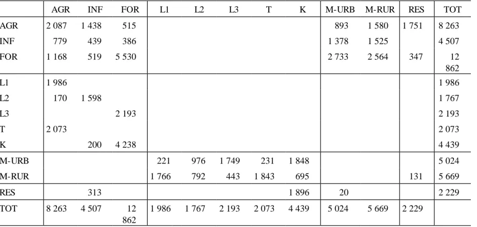
Although the model is based on information at the household level, an aggregate social accounting matrix (SAM) with 13 accounts can be derived from the source data (Table 1). In this aggregated SAM, the labor factor is disaggregated into three types of work: agricultural family work, informal wage work and formal wage work. The household account is

disaggregated into two accounts, one for urban households and the other for rural households. The formal sector account is an aggregate of private and public formal activities accounts, while the last account (RES) is an aggregate of the accounts of the formal firms, government, saving-investment and rest of the world. This matrix summarizes the model accounts, which include 4500 households, of which approximately 3500 are agricultural producers. Thus, there are thousands of household, factor, and activity accounts in the full model SAM.

Table 1: Social Accounting Matrix (billions of Francs Malgaches 1995)

AGR INF FOR L1 L2 L3 T K M-URB M-RUR RES TOT

AGR 2 087 1 438 515 893 1 580 1 751 8 263 INF 779 439 386 1 378 1 525 4 507 FOR 1 168 519 5 530 2 733 2 564 347 12 862 L1 1 986 1 986 L2 170 1 598 1 767 L3 2 193 2 193 T 2 073 2 073 K 200 4 238 4 439 M-URB 221 976 1 749 231 1 848 5 024 M-RUR 1 766 792 443 1 843 695 131 5 669 RES 313 1 896 20 2 229 TOT 8 263 4 507 12 862 1 986 1 767 2 193 2 073 4 439 5 024 5 669 2 229

L1 = agricultural family labor L2 = informal labor

5. An Application to Madagascar

Some of the microeconomic functions were estimated on cross-sectional data: the agricultural production function and the informal income equation at the household level and the formal wage equation at the individual level. On the consumption side, the parameters of the linear expenditure system and the labor supply function could not be estimated but were

calibrated using estimates found in the literature and data derived from the household survey and the SAM.

5.2. Estimation Results

The econometric techniques implemented are inspired to the extent possible by econometric work relating to household labor allocation. The complexity of the methods

implemented is nevertheless limited by the need to estimate the functions on the whole sample of households and not just on a sub-sample. Thus, in the case of the agricultural production

function, we did not differentiate the types of labor according to qualification or gender, because we did not find a well-behaved neoclassical function with satisfactory which permits null

quantities of one of the production factors. The estimation of a function with several types of work would in addition have made it possible to write the labor allocation model at the level of individuals and not of households. To our knowledge, only Newman and Gertler (1994) have implemented a complete estimation of a time allocation model for agricultural households with an arbitrary number of members. Their specification assumes nevertheless use of only part of the available information, since the model estimation relies only on the observed marginal

productivity data, i.e. wages, and uses the Kuhn-Tucker conditions to estimate the marginal productivity of on-farm family labor. The comparison of wages and productivities derived from the estimate of an agricultural production function based on the EPM93 data shows that these conditions do not hold.

Agricultural Production Function

Following Jacoby (1993) and Skoufias (1994), we considered an agricultural production function and derived the marginal productivity of agricultural labor for each household. Agricultural households are defined as all those that draw an income from land. Other agricultural factors include agricultural equipment and livestock. The search for a function making it possible to take into account null quantities of inputs led us to consider estimating a quadratic function embedded in a Cobb-Douglas function. The quadratic form makes it possible to take into account several types of work and null quantities of factors. We abandoned this approach for two reasons. One is that the estimation results are much less satisfactory from an econometric point of view. The other is that the function is much less handy analytically, which considerably complicates the writing of the model. The Cobb-Douglas has advantages in terms of interpretation and handiness. Beyond the homogeneity of family work, the assumptions related to the use of a Cobb-Douglas function are strong: the contribution of the production factors are strongly separable, and the marginal rate of substitution between factors is equal to 1 and does not depend on the other factors.

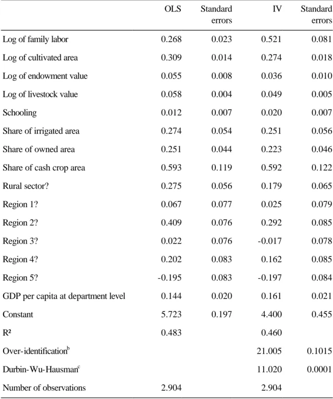
The logarithm of agricultural value added is regressed on the logarithms of the four production factors (work in hours, land in hectares, endowment in value, livestock in value), and the average level of education of the household, as well as on variables characterizing the cultivated land (share of irrigated surface, share of surface in property, share of the cultures of cash crops) and on regional dummy variables. Because of endogeneity of certain explanatory variables, the ordinary least squares estimate (OLS) is likely to give biased results. The endogeneity bias can result from the overlap of production and input allocation decisions, and from fixed effects of unobserved heterogeneity. The multiplicity of the endogeneity sources does not permit determination of the bias direction a priori. Since the capital stock, acreage and livestock are considered fixed over the period considered (one year of production) and intermediate consumptions are deduced from the value of the production - which amounts to assuming that they are complementary - the only instrumented variable is the use of family work. The instrumental variables (IV) must be correlated with the explanatory variables but not with

the residuals of the production function. The selected IV are the demographic structure of the household and the age of the household head. The results of the estimates by OLS and IV methods are presented in Table 2. The first stage of the estimate - regression of the variable instrumented on the instrumental variables - indicates that the instruments are relatively powerful in explaining the variation of the quantities of family work applied to the agricultural activity. The results of the over-identification test make it possible to reject the null hypothesis of correlation between the residuals of the IV estimate and the instruments, while the results of the Durbin-Wu-Hausman test show that the family work coefficient in the production function estimated by the IV is significantly different from the coefficient estimated by the OLS. The comparison of the results of the estimates by the OLS and the IV show that the coefficient of family work

(corresponding to its contribution in the agricultural value added) is biased towards zero in the OLS estimate, since it increases from 0.27 to 0.52. The parameters corresponding to the other production factors decrease slightly in the IV estimate, but the total sum of the contributions of the production factors increases significantly (from 0.69 to 0.88) between the two estimates. Since this value is not significantly different from 1, one can consider a constant returns to scale agricultural production technology.

Table 2: Results of estimations of the function of agricultural value added (OLS and IV) OLS Standard errors IV Standard errors

Log of family labor 0.268 0.023 0.521 0.081

Log of cultivated area 0.309 0.014 0.274 0.018

Log of endowment value 0.055 0.008 0.036 0.010

Log of livestock value 0.058 0.004 0.049 0.005

Schooling 0.012 0.007 0.020 0.007

Share of irrigated area 0.274 0.054 0.251 0.056

Share of owned area 0.251 0.044 0.223 0.046

Share of cash crop area 0.593 0.119 0.592 0.122

Rural sector? 0.275 0.056 0.179 0.065 Region 1? 0.067 0.077 0.025 0.079 Region 2? 0.409 0.076 0.292 0.085 Region 3? 0.022 0.076 -0.017 0.078 Region 4? 0.202 0.083 0.162 0.085 Region 5? -0.195 0.083 -0.197 0.084

GDP per capita at department level 0.144 0.020 0.161 0.021

Constant 5.723 0.197 4.400 0.455

R² 0.483 0.460

Over-identificationb 21.005 0.1015

Durbin-Wu-Hausmanc 11.020 0.0001

Number of observations 2.904 2.904

a The dependent variable is the log of the agricultural value added.

b Over-identification test for exclusion of instruments, Chi-square distribution under the null and associated probability.

c Durbin-Wu-Hausman test for OLS specification bias, Chi-square distribution under the null and associated probability.

Informal and Formal Wage Equations

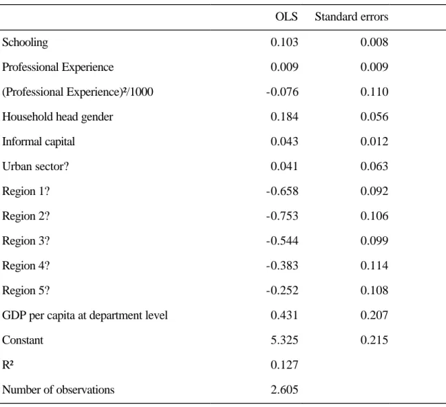
The informal wage equation was estimated at the household level (Table 3), while the formal wage equation was estimated at the individual level (Table 4).

Table 3: Results of estimations of informal wage equation at the household level

OLS Standard errors

Schooling 0.103 0.008

Professional Experience 0.009 0.009

(Professional Experience)²/1000 -0.076 0.110

Household head gender 0.184 0.056

Informal capital 0.043 0.012 Urban sector? 0.041 0.063 Region 1? -0.658 0.092 Region 2? -0.753 0.106 Region 3? -0.544 0.099 Region 4? -0.383 0.114 Region 5? -0.252 0.108

GDP per capita at department level 0.431 0.207

Constant 5.325 0.215

R² 0.127

Number of observations 2.605

The independent variables are the logarithms of the wage rates. Only the results of the OLS estimates were retained. The results of the estimates according to the Heckman procedure showed that there is no observable selection bias.

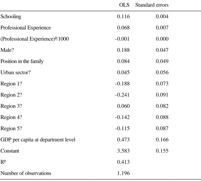
Table 4: Results of estimations of formal wage equation at the individual level

OLS Standard errors

Schooling 0.116 0.004

Professional Experience 0.068 0.007

(Professional Experience)²/1000 -0.001 0.000

Male? 0.188 0.047

Position in the family 0.084 0.049

Urban sector? 0.045 0.056 Region 1? -0.188 0.073 Region 2? -0.241 0.091 Region 3? 0.060 0.082 Region 4? -0.142 0.088 Region 5? -0.115 0.087

GDP per capita at department level 0.473 0.166

Constant 3.583 0.155

R² 0.413

Number of observations 1.196

The performances of the two regressions in terms of explaining the variance are relatively poor for the informal wage equation (R²=12.7%) and relatively good for the formal wage equation (R²=41.3%). Nevertheless, the results show that the coefficients of the human capital variables have the expected signs in the two equations: the returns to education are positive and significant and the returns to experience are positive in the two regressions but significant only in the second. The sign of the parameter of experience squared (introduced to take into account the decreasing returns to experience) is negative and significant in the formal wage regression. In addition, the outputs of education appear 5 times higher in the informal sector than in the agricultural sector. The coefficient of the gender variable (of the head of

household in the case of the informal wage equation, and of the individual in the formal wage equation) is significant and positive, indicating that men have a significantly higher average wage rate than that of the women in the two sectors.

5.3. Calibration, Parameters and Algorithm

Calibration is a traditional stage in the construction of applied models, in particular in constructing general equilibrium models. In our model, calibration procedures are of several types. Initially, the reconciliation of the microeconomic data of 1993 with the macroeconomic data of 1995 was carried out using a program of recalibration of the statistical weights

(Robilliard and Robinson, 1999). "Traditional " procedures of calibration were implemented to calibrate the parameters of the demand system, labor supply and the transformation function. The partially random drawing of potential and reservation wages is “non traditional” and constitutes an innovative step, characteristic of the microsimulation models with endogenous microeconomic behaviors.

Parameter Calibration

The linear expenditure system (LES) was calibrated for each household given the budgetary shares derived from the household data and the SAM, the income elasticity of the agricultural and formal demands, and the Frisch parameter. The price elasticities and the LES parameters were derived from the calibration process. The outcome of this process is that minimal expenditures are specific to each household, as are propensities to consume supernumerary income. This specification leads to individual demand functions whose

aggregation is not perfect, i.e. whose aggregate cannot be described through a function of the same type as the individual function. Only a specification based on marginal propensities to consume supernumerary income equal for all the households allows perfect aggregation (Box 1).

Box 1 : LES Calibration and perfect aggregation

Following Deaton and Muellbauer (1980), the Linear Expenditure System writes

(

−

_∑

)

+ = _{i i i j j} i iq p x p p γ β γ with

∑

βj =1 where q i _{consumption of good i}

x expenditures

i

γ _{subsistence consumption}

i

β _{marginal propensity to consume supernumerary expenditure.}

LES parameter calibration requires (Dervis and al., 1982) the knowledge of income elasticities of the demand for each good

( )

εi _{, of the Frisch parameter}

( )

φ _{, and of budget shares}

( )

ωi _.

One can show that: βi =εiωi

Given that −

∑

− = j j p x x γ φ

One can show that 

   ₊     = φ β ω γ i i i i p x

Consider q , the consumption of good i oh household h. The LES of household h is: ih

(

−

∑

)

+ = _{i ih ih h j jh} ih iq p x p p γ β γ

Aggregate consumption is the sum of individual consumptions and can be written:

(

)

∑

∑

∑

∑

= + − = h jh j h ih h ih i h ih i i iq p q p x p p γ β γ

Aggregation is perfect, that is, aggregate consumption can be written:

(

−

∑

)

+ = _{i i i j j} i iq p x p p γ β γ with

∑

= h ih i γ γ and

∑

= h h x x if and only if βih = βih′ =βi_.

The labor supply function was calibrated for each household given the price and income elasticities drawn from Jacoby (1993). The savings function was calibrated given the income elasticity of the marginal propensity to save. Finally, the autonomous agricultural demand was calibrated given the price elasticity of demand. Other calibrations include incomes derived from sharecropping and formal capital.

agricultural goods produced for the local market and those produced for export. The

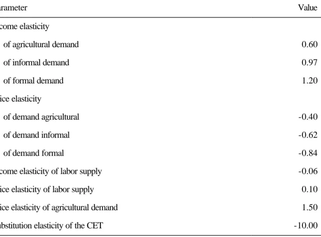
formalization of this assumption is based on the specification of a function with constant elasticity of transformation (CET) for each agricultural household. The calibration of the CET function is based on the production data derived from the household survey but also requires the definition of the substitution elasticity between production for the local market and exports. For this parameter, which cannot be estimated because of the absence of a long series of data on production and price, an "average" value, was selected. Thereafter, various simulations were carried out to test the sensitivity of the results of the model to the value of this parameter. The values of "guesstimated" parameters of the reference simulation are presented in Table 5.

Table 5: Model Parameters

Parameter Value Income elasticity of agricultural demand 0.60 of informal demand 0.97 of formal demand 1.20 Price elasticity of demand agricultural -0.40 of demand informal -0.62 of demand formal -0.84

Income elasticity of labor supply -0.06

Price elasticity of labor supply 0.10

Price elasticity of agricultural demand 1.50

Potential Wage Equation

In order to model the labor allocation choices and hiring in the formal sector, it is necessary to know the potential informal and formal wages for households and individuals who do not take part in the labor market being considered. The estimation of these wages is carried out on the basis of the results of the econometric estimations presented earlier. From these estimations one can compute informal (for each household) and formal (for each individual) potential wages given their specific levels of human capital and the values of the other

explanatory variables of the regression. The next step consists of drawing the residuals, which represent the fixed effects. In the case of informal wages, this drawing is carried out under two assumptions. The first relates to the distribution of the residuals, which is assumed to be normal. The second relates to the labor allocation model for the agricultural households, with which the values of the informal potential and reservation wages must be consistent. The potential and reservation wage residuals are drawn under the condition that the marginal productivity of agricultural labor, i.e. the shadow wage of agricultural labor, is higher than the potential informal wage corrected by the reservation wage. In the case of the drawing of informal wages residuals for nonagricultural households and individual formal wages, only the assumption of normal distribution is retained.

Equations and Heterogeneity

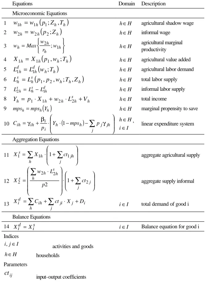
The microeconomic and macroeconomic equations of the model are presented in Table 6.

Table 6: Model Equations

Equations Domain Description

Microeconomic Equations

1

w

_1h

=

w

_1h

(

p

₁

;

Z

_h

,

T

_h

)

h∈H agricultural shadow wage 2

w

_2h

=

w

_2h

(

p

₂

;

Z

_h

)

h∈H informal wage 3       = _h h h h w r w Max w 2 ; ₁ h∈H agricultural marginal productivity

4

X

_1h

=

X

_1h

(

p

₁

,

w

_h

;

T

_h

)

h∈H agricultural value added 5

L

₁d_h

=

L

₁d_h

(

w

_h

;

T

_h

)

h∈H agricultural labor demand 6

L

_hs

=

L

s_h

(

p

₁

,

p

₂

,

w

_h

;

T

_h

,

Z

_h

)

h∈H total labor supply

7 Ls_2h = L_hs −Ld_1h h∈H informal labor supply 8

Y

_h

=

p

₁

⋅

X

_1h

+

w

_2h

⋅

L

s_2h

+

V

_h h∈H total income

9 mps_h =mps Y_h

( )

_h h∈H marginal propensity to save

10

(

)

_       − − ⋅ ⋅ + =

∑

j jh j h h i i ih ih Y mps p p C γ β 1 γ h∈H,

i∈I linear expenditure system

Aggregation Equations 11

∑

∑

_       + ⋅ = h j jh h s ct X

X_{1 1} 1 ₁ aggregate agricultural supply

12 _       + ⋅             _⋅ =

∑

∑

j j h s h h s _ct p L w X ₂ 2 2 2 1

2 aggregate supply informal

13 i j j ji h ih d i C ct X D X =

∑

+

∑

⋅ +

i∈I total demand of good i Balance Equations

14 X_id = X_is i∈I Balance equation for good i

Indices

i j, ∈I _{activities and goods} h∈H _households

Parameters

ct

γ βih, i _{LES parameters for good i and household h}

h

r reservation wage labor off farm of household h

h

T

characteristics of agricultural farm of household h (land, capital livestock...)

h

Z

_{characteristics of household h (size, demographic composition, education,,,)}

Variables

i

p

_{price of i}

w_{1h shadow wage of on-farm family labor of household h}

h

w

_{2 informal wage of household h}

h

w

wage of household h s h

L

total labor supply of household h

d h

L

_{1 agricultural labor demand of household h}

s h

L

_{2 informal labor supply of household h}

h

X

₁

agricultural value added of household h

h

Y

_{income of household h}

h

mps

_{marginal propensity to save of household h}

ih

C

consumption of good i of household h

i

D

_{autonomous demand of i} s i

X

aggregated supply of i d i

X

aggregated demand of i

The model takes into account various sources of heterogeneity at the household level. These differ by their demographic characteristics, by their endowments in physical and human capital, by their position on the labor market, and by their preferences of consumption and labor supply. The conservation of the residuals in the microeconomic equations makes it possible to take into account unexplained elements of heterogeneity.

Algorithm and Solution

The model was written using the GAUSS software. The solution algorithm is a loop with decreasing steps that seeks the equilibrium prices that will clear excess demands for the

agricultural good and informal labor. At each step, all the microeconomic functions of behavior are recomputed with new prices. Since the process of labor allocation for agricultural

households is discrete, these can " switch " from a state of autarky (where they do not take part in the wage labor market) to a state of multi-activity, according to the respective values of the implicit on-farm wage (which depends on the price of the agricultural good) and of the

corrected market wage (which depend on the price of informal labor). The individual demands and supplies are then aggregated to obtain the functions of excess demand that one seeks to clear. Solution time depends on the magnitude of the shocks and computational capacities available. As an example, the time varies between 1 and 5 minutes for the shocks considered in this paper on a Penthium 450 with 128 MB of read-write memory.

6. Impact of Growth Shocks on Poverty and Inequality

The first set of simulations relates to various growth shocks, corresponding to various development strategies. The impact of these various shocks on poverty and inequality is analyzed. The comparative statics of the model is studied through the analysis of the results at the aggregate level. The ex ante / ex post decomposition of the results makes it possible to emphasize the importance of the general equilibrium effects, while reading the microeconomic results through a detailed classification of households makes it possible to evaluate the contribution of endogeneizing the within-group variance of income. Some results of sensitivity tests for "guestimated" parameters are also presented.

6.1. Some Descriptive Elements

Ménages) survey of 1993. a national survey of the SDA type (social dimension of adjustment) covering 4508 households. This survey was carried out by the INSTAT (Institut National de la Statistique) on behalf of the Malagasy government. The macroeconomic data correspond to those of the Social Accounting Matrix of Madagascar for the year 1995 (Razafindrakoto and Roubaud, 1997). This SAM, in addition, was used as the base for a computable general

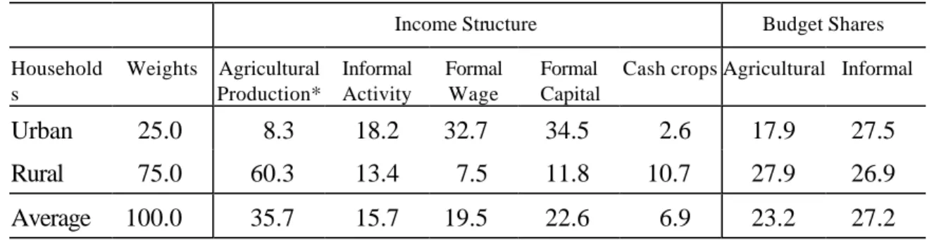
equilibrium model applied to Madagascar (Dissou, Haggblade and al., 1999). The reconciliation of the microeconomic data of 1993 with the macroeconomic data of 1995 was carried out using a program of recalibration of the statistical weights (Chapter 5). The results of the model thus correspond to the Malagasy economy of 1995 and are presented in constant 1995 Francs Malgaches. The figures in Table 7 show that the income structure differs greatly between rural households, whose incomes are dominated by agricultural production, and urban households, whose incomes are dominated by formal production factors. The consumption patterns also differ since the agricultural budget share is 17.9% in the urban sector and 27.9% in the rural sector.

Table 7: Household income and consumption structure (%)

Income Structure Budget Shares

Household s Weights Agricultural Production* Informal Activity Formal Wage Formal Capital

Cash crops Agricultural Informal

Urban 25.0 8.3 18.2 32.7 34.5 2.6 17.9 27.5

Rural 75.0 60.3 13.4 7.5 11.8 10.7 27.9 26.9

Average 100.0 35.7 15.7 19.5 22.6 6.9 23.2 27.2

Source: EPM93. authors' calculations. * including cash crops.

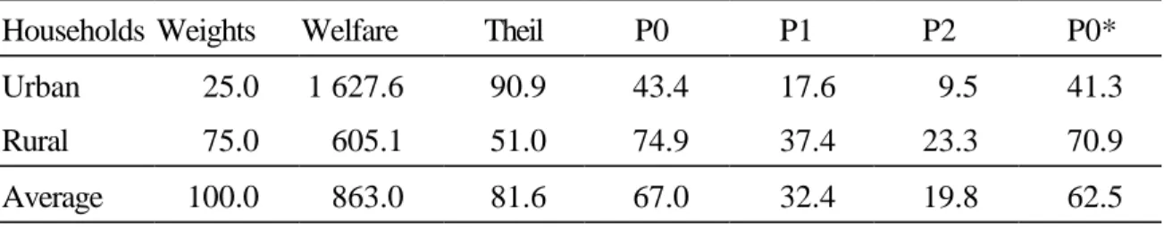
Table 8 presents various indicators of poverty and inequality as well as the distribution of the poor between the rural and urban sector.

Table 8: Poverty and Inequality

Households Weights Welfare Theil P0 P1 P2 P0*

Urban 25.0 1 627.6 90.9 43.4 17.6 9.5 41.3

Rural 75.0 605.1 51.0 74.9 37.4 23.3 70.9

Average 100.0 863.0 81.6 67.0 32.4 19.8 62.5

Source: EPM93. authors' calculations.

Several indicators are used for this descriptive analysis and will be used again for the analysis of the results. The three indicators of poverty depend on the definition of a poverty line. Following several analyses of poverty in Madagascar, we took the per capita "caloric" line which corresponds to the poverty line used at the national level and which amounts to 248.000 1993 Francs Malgaches. This threshold corresponds to a per capita income sufficient to buy a minimum basket of basic foodstuffs (representing a ration of 2.100 Kcal per day) and of non-food staples. The first indicator (P0) is that of the poverty rate. It corresponds to the share of the population living below the poverty line, but does not inform about the degree of poverty. The second indicator is that of poverty depth (P1), where the contribution of each individual to the aggregate indicator is larger the poorer this individual. The third indicator is the severity of the poverty (P2), which is sensitive to inequality among the poor. Regarding income distribution, only the Theil index was retained as an indicator of inequality, because of its properties. It is a decomposable indicator, which makes it possible to consider the respective contributions of within and between-group inequality to total inequality. According to these indicators and the chosen poverty line, 67.0% of the population is poor in Madagascar. The poverty rate is higher in the rural sector where it reaches 74.9% of the population. The depth and severity of poverty are also higher in the rural sector. On the other hand, inequality is higher in the urban sector. Although the average income of the urban households is 2.7 times higher than that of the rural households, the between-group inequality accounts for only 15% of the overall inequality.

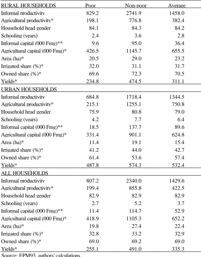
informal activities. Other characteristics, not observed, also contribute to heterogeneity among the households. Average informal labor productivity is computed for all households, since the estimate of informal wages enables us to calculate potential standards of informal wages for households for which these wages are not observed. Agricultural productivity is calculated only for the agricultural households, because this activity is related to a fixed factor, land.

Table 9: Structural characteristics of Malagasy households

RURAL HOUSEHOLDS Poor Non-poor Average

Informal productivity 829.2 2741.9 1458.0

Agricultural productivity* 198.1 776.8 382.4

Household head gender 84.1 84.3 84.2

Schooling (years) 2.4 3.6 2.8 Informal capital (000 Fmg)** 9.6 95.0 36.4 Agricultural capital (000 Fmg)* 426.5 1145.7 655.5 Area (ha)* 20.5 29.0 23.2 Irrigated share (%)* 32.0 31.1 31.7 Owned share (%)* 69.6 72.3 70.5 Yields* 234.8 474.5 311.1 URBAN HOUSEHOLDS Informal productivity 684.8 1718.4 1344.5 Agricultural productivity* 215.1 1255.1 750.8

Household head gender 75.9 80.8 79.0

Schooling (years) 4.2 7.7 6.4 Informal capital (000 Fmg)** 18.5 137.7 89.6 Agricultural capital (000 Fmg)* 331.4 901.1 624.8 Area (ha)* 11.4 19.1 15.4 Irrigated share (%)* 41.2 44.0 42.7 Owned share (%)* 61.4 53.6 57.4 Yields* 487.8 574.3 532.4 ALL HOUSEHOLDS Informal productivity 807.2 2340.0 1429.6 Agricultural productivity* 199.4 855.8 422.5

Household head gender 82.9 82.9 82.9

Schooling (years) 2.7 5.2 3.7 Informal capital (000 Fmg)** 11.4 114.7 52.9 Agricultural capital (000 Fmg)* 418.9 1105.3 652.2 Area (ha)* 19.8 27.4 22.4 Irrigated share (%)* 32.8 33.2 32.9 Owned share (%)* 69.0 69.2 69.0 Yields* 255.1 491.0 335.3

Source: EPM93. authors' calculations.

* average computed on agricultural households. ** average computed on informal households.

Not surprisingly, poor households are characterized by low labor productivity in the two traditional sectors. The weakness of these levels of productivity is related to low levels of endowments in human and physical capital. Poor households’ levels of education (measured in years of schooling) are nearly 2 times lower than those of non-poor households, and their average level of informal capital (measured in value for the households which have an informal activity) is 10 times lower. Surprisingly, the informal labor productivity appears higher in the rural sector than in the urban environment, in spite of lower levels of endowment in human and physical capital. The parameter of the dummy variable for the urban sector is not significantly different from zero in the equation of informal income. This result can nevertheless be explained by the shortage of formal goods in the rural sector, for which informal activities may be

substituted. The endowment of production factors of the urban households is higher overall, except with regard to the agricultural endowment.

6.2. Description of the Growth Shocks

Several strategies of development can be considered for the Malagasy economy: either continuation of a formal sector "push", through development of the "Zone Franche", or the massive investment in the development of the agricultural sector which suffered from underinvestment during the last decades and whose performance is poor. In the agricultural sector, efforts can be focused either on tradable crops (cultivation of cash crops, coffee-vanilla-clove), which are traditional exports of Madagascar, or on non-tradable food crops (rice, corn, manioc, pulses).

Table 10: Simulations Table

Simulation Description

EMBFOR Formal hiring and increase in dividends SALFOR Increase in formal wages and in dividends

PGFAGRI Increase of the Total Factor Productivity in the agricultural sector PGFALIM Increase of the Total Factor Productivity in the food-crop sector PGFRENT Increase of the Total Factor Productivity in the cash-crop sector PRXRENT Increase of the world price of cash crops

The first two simulations relate to an increase in formal sector value added. Given the model structure, formal value added comes from two production factors. In the first simulation (EMBFOR), formal sector growth corresponds to the creation of new companies and thus to an increase in the capital stock and employment. It is simulated through an increase in income coming from dividends for shareholders, and from formal labor demand. This increase is simulated through the sampling of individuals from the non-working and non-formal working population. The hiring schema is partially random. Its structure is defined in terms of gender, age, education, and sector (rural/urban). This structure was derived from the household data and corresponds to the structure of formal employment during the last five years. In addition, individuals whose agricultural or informal incomes are higher than their potential formal wages are excluded from the drawing. Lastly, all sampled individuals are employed on a full-time basis whatever their former level of occupation. Consequently, if an individual is hired in the formal sector, less time but more exogenous income is available at the household level.

In the second simulation (SALFOR), value added paid to formal labor increases through a formal wage increase but with no effect on employment. The value added of formal capital increases as in the preceding simulation. The direct effect of this shock is an increase in the incomes of households receiving formal wages. Compared to the preceding simulation, one can expect that the effects on poverty and inequality will be less favorable.

The following simulations relate to the agricultural sector. The first simulation

(PGFAGRI) considers an increase in total factor productivity for all agricultural households. This leads to an increase in agricultural income and agricultural production. In the next simulation (PGFALIM), the increase in productivity relates to only food production. The last two

simulations relate to cash crops. In simulation PGFRENT, we examine the effect of an increase in the productivity of cash-crop production. In PRXRENT, we simulate the impact of an increase in cash-crop world prices. In both cases, a positive impact on the agricultural terms of trade is expected.

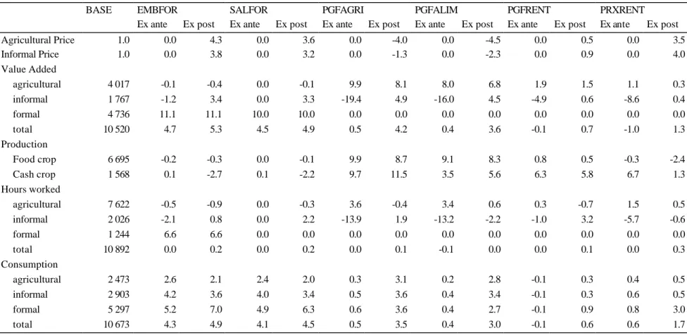
6.3. Ex ante / Ex post Decomposition of the Impact of Growth Shocks

In order to emphasize the contribution of the general equilibrium framework, we present the results of simulation ex ante and ex post (Table 11 to 13). The ex ante results correspond to the results of a microsimulation model with microeconomic behaviors and fixed prices, whereas the ex post results correspond to a microsimulation model with microeconomic behaviors and endogenous relative prices.

In the first simulation (EMBFOR), the hiring shock decreases the quantity of working time available for the traditional activities, which, ex ante, leads to a reduction in the agricultural (-0.1%) and informal (-1.2%) value added. At the same time, the increase in available income (+4.3%) leads to an increase in the demand for consumer goods. The combination of a lower production and an increase in consumption is likely to lead to an increase of relative prices of traditional goods. This is what we can observe ex post, where the prices of the traditional goods increase by 4.3% for the agricultural food crop and by 3.8% for the informal good. This change in relative prices of agricultural and informal goods determines the effect on the real income of each household, according to the structure of its income and consumption. Ex ante, the effect of the shock on inequality is negative: the Theil index increases by 3.0%. The increase in inequality is stronger in the rural (+4.7%) than in urban sector (+1.6). The between-group inequality also increases (+2.8%). Ex post, the situation is relatively different because of income effects for

non-formal households through the increase of relative prices of traditional goods. This mechanism does not affect the extent of the welfare shock but does affect its distribution. The increase in per capita income is actually stronger in the rural sector than in the urban

environment, which induces a reduction in between-group inequality (-3.2%). This reduction, however, does not compensate for the increase in within-group inequality (+1.4%) and, overall, inequality measured by the Theil index increases by 0.8%. The combination of the average income per capita growth (+5.0% ex post) and the fall in inequality leads to a reduction in the rate (-2.6%) and depth of poverty (-4.3%), as well as its severity (-5.1%) in both urban and rural sectors.