Differences between repeated borehole temperature logs in the southern Canadian Prairies-validating borehole climatology

(1)

HAL Id: hal-00298160

https://hal.archives-ouvertes.fr/hal-00298160

Submitted on 7 Nov 2006

HAL is a multi-disciplinary open access

archive for the deposit and dissemination of sci-entific research documents, whether they are pub-lished or not. The documents may come from teaching and research institutions in France or abroad, or from public or private research centers.

L’archive ouverte pluridisciplinaire HAL, est destinée au dépôt et à la diffusion de documents scientifiques de niveau recherche, publiés ou non, émanant des établissements d’enseignement et de recherche français ou étrangers, des laboratoires publics ou privés.

Differences between repeated borehole temperature logs

in the southern Canadian Prairies-validating borehole

climatology

J. Majorowicz, W. Skinner, J. Safanda, W. Gosnold

To cite this version:

J. Majorowicz, W. Skinner, J. Safanda, W. Gosnold. Differences between repeated borehole temper-ature logs in the southern Canadian Prairies-validating borehole climatology. Climate of the Past Discussions, European Geosciences Union (EGU), 2006, 2 (6), pp.1075-1104. �hal-00298160�

(2)

CPD

2, 1075–1104, 2006 Repeated borehole temperature logs J. Majorowicz et al. Title Page Abstract Introduction Conclusions References Tables Figures J I J I Back Close

Full Screen / Esc

Printer-friendly Version Interactive Discussion

EGU

Clim. Past Discuss., 2, 1075–1104, 2006 www.clim-past-discuss.net/2/1075/2006/ © Author(s) 2006. This work is licensed under a Creative Commons License.

Climate of the Past Discussions

Climate of the Past Discussions is the access reviewed discussion forum of Climate of the Past

Di

fferences between repeated borehole

temperature logs in the southern

Canadian Prairies-validating borehole

climatology

J. Majorowicz1,4, W. Skinner2, J. Safanda3, and W. Gosnold4

1

Northern Geothermal, 105 Carlson Close, Edmonton, Alberta, T6R 2J8, Canada

2

Climate Research Division, Environment Canada, Toronto, Ontario, M3H 5T4, Canada

3

Geophysical Institute, Prague, Czech Republic

4

University of North Dakota, Northern Plains Climate Research Centre, Grand Forks, ND, USA Received: 25 October 2006 – Accepted: 29 October 2006 – Published: 7 November 2006 Correspondence to: J. Majorowicz (majorowicz@shaw.ca)

(3)

CPD

Full Screen / Esc

EGU

Abstract

Temperature-depth (T-z) profiles from twenty-four shallow boreholes of less than 250 m in depth located in flat, semi-arid areas of the southern Canadian Prairie Provinces initially measured in the late 1980’s and early 1990’s and repeated between 2004 and 2006 show strong ground surface temperature (GST) warming signatures. GST

5

changes of 0.1–0.2◦C, and 0.4◦C, are observed between the measurements for the shorter (decade) and longer (two decades) time spans, respectively. Borehole sites with repeated temperature logs are selected to demonstrate that multiple T-z profiles provide general agreement between GST warming and observed surface air temper-ature (SAT) warming measured at nearby historical climate stations. A comparison

10

of measured changes from repeated temperature logs with those simulated from SAT forcing demonstrates the influence of SAT on the observed deviation of temperature with depth despite variations in snow cover. Repeated borehole measurements from the northern Great Plains of the USA also identify a similar positive temperature change but of lower magnitude. Temperature changes since 1900 in the southern Canadian

15

Prairies and the adjoining northern Great Plains of the USA, as derived from the func-tional state inversion (FSI) of deeper borehole logs, average 2.5◦C but show a strong latitudinal gradient.

1 Introduction

The southern Canadian Prairie region has been experiencing one of the highest mean

20

annual surface air temperature (SAT) and ground surface temperature (GST) increases measured in the Northern Hemisphere. Increases in annual SAT from 1950 to 1995 have ranged from 0.5 to 2.5◦C across this region (Zhang et al., 2000). In addition, there has been an even larger GST warming across this region between 1.5 and 4.0◦C over the past century (Majorowicz et al., 1999). Previous borehole climate studies in the

25

(4)

CPD

Full Screen / Esc

EGU

Skinner and Majorowicz, 1999) have confirmed that SAT forcing is largely responsible for the GST warming. The average amplitude of GST warming throughout North Amer-ica, based on greater than 500 available temperature logs, including Alaska, the Cana-dian Arctic and the CanaCana-dian Prairies is 0.95◦C (SE=0.05◦C) beginning approximately 220 years ago (SE=8.5 years) (Majorowicz et al., 2006b1). Average GST warming, as

5

derived from well temperatures, is approximately 0.4◦C greater than SAT warming as derived from published proxy sources as well as observational records over the same period (Majorowicz et al., 2006b1).

The coherence between GST warming, as reconstructed from borehole temperature-depth (T-z) profiles, and SAT warming has been questioned (Mann et al., 2003),

es-10

pecially for northern locations where seasonal snow cover exists. Snow cover magni-tude could explain some of the misfit between SAT and GST records (Todhunter et al., 2005). The magnitude of the difference between the mean annual SAT and GST at a given site varies according to the number of days with snow cover or the content of soil moisture at the beginning of the freezing season. The GST’s are normally higher than

15

the SAT’s as the snow cover insulates the subsurface from temperatures below 0◦C (Lachenbruch, 1994; Stieglitz et al., 2003). The difference, however, can be relatively insensitive to the depth of the snow layer (Schmidt et al., 2001). It has been shown through long-term observation at the same location over many years that mean annual GST’s closely correlate with mean annual SAT’s in the north-central USA for 1963–

20

1990 (Baker and Ruschy, 1993), and in both northern (boreal forest) and southern (grassland) Alberta locations for 1965–1990 (Majorowicz and Skinner, 1997).

Water flow in the recharge – discharge areas can also influence subsurface tempera-ture (Reiter, 2005; Ferguson and Woodbury, 2005). However, recent analysis of water seepage velocities done in the Alberta Basin provides proof that they are too small

25

(approximately 5 mm/yr) to effect T-z profiles (Majorowicz et al., 2006a). High GST

1

Majorowicz, J. A., Skinner, W. R. and Safanda, J.: Variability in the onset of post-Little Ice Age warming across North America as inferred from borehole temperature logs, Clim. Past Discuss., in preparation, 2006b.

(5)

CPD

Full Screen / Esc

EGU

warming in the North American mid-continent has been driven by a large SAT warming over the past two centuries (Majorowicz et al., 1999; Harris and Gosnold, 1999). Also, it has been shown that the effects of permanent land clearing in some regions formerly covered with forests (central Alberta) can superimpose an additional step-like increase of GST upon a climate warming signal (Skinner and Majorowicz, 1999). Deforestation

5

(Lewis, 1998; Lewis and Skinner, 2003) and large forest fires (Majorowicz and Skinner, 1997) can also affect GST changes.

There are three basic assumptions made in the reconstruction of ground surface temperature history (GSTH) from T-z logs. The first is the GST systematically couples with the SAT, the second is there is a constant offset between the mean annual GST

10

and SAT at each well site on multiyear to decadal time scales, and the third is the surface temperature variations diffuse by conduction into the subsurface and impose a transient “climate” signal on the steady-state geothermal gradient.

The purpose of this study is to compare T-z profiles recorded in the same bore-holes at different times over one to two decades with data from nearby climate

sta-15

tions. Results of temperature measurements with depth for 24 borehole sites lo-cated in the Western Canadian Sedimentary Basin, in central and southern Alberta and south-central Saskatchewan are presented. Comparisons are made between ob-served changes in T-z profiles over time with the synthetic temperature profiles gener-ated using the SAT forcing from nearby Canadian and USA Historical Climate Network

20

stations. Snow cover records from three Canadian Historical Climate Network stations in the southern Canadian Prairies are also analyzed in conjunction with the period of well re-logging to assess the effects of snow cover on GST. Also, comparisons are made with T-z profiles from the geographically adjacent northern Great Plains of the USA (Gosnold et al., 1997).

(6)

CPD

Full Screen / Esc

EGU

2 Study area and data

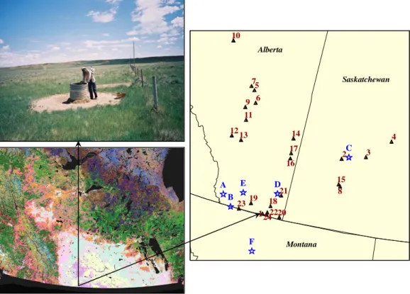
The study area of central and southern Alberta and south-central Saskatchewan is located entirely in the Western Canadian Sedimentary Basin. Figure 1 shows the ge-ographic location of the 24 wells. Figure 1 also shows an example photograph of a well site located in southern Alberta close to the Montana border and depicts a typical

5

surface landscape surrounding the majority of the sampled wells. All wells, with the ex-ception of well #10, are located within the Prairie Ecozone (Fig. 1) and are surrounded by either flat grassland used for grazing or flat agricultural cropland. Well #10 is lo-cated in north-central Alberta in the Boreal Plains Ecozone (Fig. 1) and is surrounded by boreal forest. Table 1 provides further information on well site name, location, initial

10

log and re-log years, and terrain type.

Repeated temperature logs were taken in twenty-four the wells shown in Fig. 1 and Table 1. All wells were initially drilled prior to 1980 for piezometric water level monitoring and have been left undisturbed for decades. Portable logging equipment was used with a thermistor probe calibrated to 0.01◦C (relative change) and 0.03◦C (absolute change)

15

with an error of depth reading of 0.1 m. The probe was attached to a 500 m cable on a portable manually operated winch and temperature was measured at discrete 2 m intervals (5 m for the oldest logs). This ensures that thermal equilibrium exists between the water in the well and the surrounding rock mass. The small well diameter relative to the length disallows any convection in the well bore significant enough to disturb the

20

thermal regime (Jessop, 1990), although circulation in an air column above the water level in the well likely exists. All measurements were taken in late Summer – early Fall. Figure 1 in the Appendix show the results of these measurements for all twenty-four wells.

The surface air temperature (SAT) data used in calculations of the synthetic response

25

for the comparison with temperature transients came from the Canadian Historical Cli-mate Network (HCN) database (Vincent and Gullett, 1999) with recent updates. The annual SAT time series used for northern Montana was an ensemble from seven USA

(7)

CPD

Full Screen / Esc

EGU

Historical Climate Network (USHCN) sites from the northern portion of the state used by Gosnold et al., 2005. Historical SAT data represent measurements originally made at airports or agricultural stations. Instrument compounds are located over natural grassed surfaces to maintain national observing consistency. Changes in the imme-diate vicinity of the instruments have been considered and adjustments have been

5

made to ensure time series homogeneity. In general, the surface characteristics imme-diately surrounding the instruments are not necessarily representative of the broader regional landscape characteristics that the temperature series are designed to repre-sent, especially in forested regions. In contrast, GST data have different site obser-vational characteristics. They are located in natural areas where use and

land-10

cover changes have occurred over the past century. The SAT pre-observational mean (POM) was used as input to the SAT-POM model of surface forcing. Snow cover data used to examine the effects of seasonal snow cover on subsurface temperatures were also taken from the Canadian Historical Climate Network (HCN) database (Mekis and Hogg, 1999). Daily snow amounts have been adjusted to account for site and

instru-15

ment changes, wind undercatch, evaporation, and trace amounts. Figure 1 shows the climate station locations used in this study. Table 2 provides further climate station information on name, location, and data used in this study.

3 Method

Rock chip and well log derived net rock lithology and rock conductivities of the Western

20

Canadian Sedimentary basin (Beach et al., 1987; Jessop, 1990) were used for ther-mal conductivity estimates (see Majorowicz et al., 1999 for details of the procedure). Transient subsurface temperature changes can be simulated by using the SAT series based on the assumption that the mean difference between the ground and air temper-atures is constant through time. Annual means (T_i) of SAT as a ground surface forcing

25

function are considered. A pre-observational mean (POM) SAT needs to be assumed for the period prior to SAT monitoring. In this study it is the average of annual SAT for

(8)

CPD

Full Screen / Esc

EGU

the 1895 to 1910 period, the earliest 16-year period of the SAT records.

The forcing function consists of a series of N jumps of amplitude ∆T_i=T_i−T_i₋₁ at times t_i before the borehole temperature measurement. The subsurface temperature response T to this forcing at depth z is

T (z)= N X i=1 ∆Ti ∗ erfc (z/ p 4kti ) 5

Where, k is thermal diffusivity and erfc is the complementary error function (Carslaw and Jaeger, 1959). This calculation depends on one free parameter, namely on the mean long-term temperature T_obefore the first change at time t₁. The parameter T_ois the pre-observational mean (POM).

Temperature differences between the repeated loggings in a well are plotted as the

10

calculated difference between the temperature profiles measured at the different times (such as 1986 and 2005). In addition, temperature differences are plotted, independent of the borehole measurements, as synthetic profiles based on the SAT – POM forcing model derived from the SAT data series at the nearby HCN stations. Transient com-ponents in boreholes are obtained as a posteriori FSI transients (for Functional Space

15

Inversion description see Shen and Beck, 1991), and as synthetic transients based on SAT time series from the nearby HCN station. The synthetic curves are calculated for assumed POM – equal to the 1895–1910 average. The thermal diffusivity used in cal-culating the synthetic curves was the same as for the FSI’s, 0.6–0.8×10−6m2s−1. The thermal conductivity model, based on lithology description and the literature (Jessop,

20

1990) assumes a thermal conductivity and specific heat of 2 MJ/(Km3). In-depth details of the method can be found in Majorowicz and Safanda (2005).

4 Results

Appendix Fig. 1 shows the results of the repeated measurements in the twenty-four southern Canadian Prairie boreholes. Four wells, Gull Lake (#11), Sundre (#12),

(9)

CPD

Full Screen / Esc

EGU

hurst T9C (#14) (also Fig. 5a), and Riverhurst T8C (#8) (also Fig. 5b) show differences much greater than 0.05◦C. Well TSA1 (#15) shows cooling from 1995 to 2005. Well TSA6 (#19) shows slight cooling from 1993 to 2005. The Gull Lake well (#11) shows very slight cooling in the proximity of the lake from 1991 to 2004. The Sundre well (#12) is a very shallow well and shows slight cooling from 1991 to 2004 likely due to

5

the hydrodynamic effect. The Saskatoon climate station is over 100 km away from the remote Riverhurst sites. SAT conditions around the well sites may be slightly modified in proximity to the man-made Lake Diefenbaker.

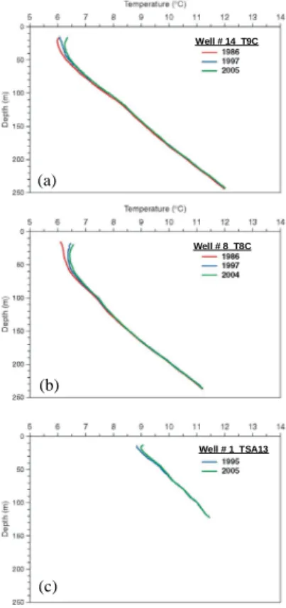
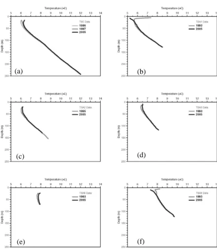
Figure 2 provides examples from deep (>100 m) re-logged wells in the semi-arid southern Canadian Prairies. Figure 2a (Well #14 T9C) is a grassland site located in

10

eastern Alberta near the Saskatchewan border and was logged first in 1986, again in 1997, and again recently in 2005. Figure 2b (Well #8 T8C) is also a grassland site and located in southern Saskatchewan and was logged first in 1986, again in 1997, and again recently in 2004. Figure 2c (Well #1 TSA13) is located in southern Alberta near the Montana border and was first logged in 1995 and again recently in 2005. These

15

wells are in thermal equilibrium as two to three decades passed since the initial drilling disturbance. There has been progressive warming with time in all three wells which is identified in accordance with conductive heat diffusion. All wells were drilled between 1977 and 1990, providing at least three years before the first temperature logs were taken. This is more than sufficient time to attain thermal equilibrium after the drilling

20

process which involved fluid circulation (Jessop, 1990). Changes in GST of 0.1–0.4◦C are observed between the measurements for the shorter (decade) and longer (close to two decades) time spans, respectively.

Figure 3 shows the annual surface air temperatures (sat) for four stations located in proximity to selected sample wells, for well #1 TSA13 to correspond to Pincher Creek,

25

Alberta (3a), an ensemble of five climate station records from Northern Montana (3b), Carway, Alberta (3c), and for well #8 T8C and well #14 T9C to correspond to Saska-toon, Saskatchewan (3d). Saskatoon was the closest high quality long range at series available is approximately 100 km distance from wells T8C and T9C these wells are

(10)

CPD

Full Screen / Esc

EGU

located in a grassland region of southern Saskatchewan in proximity to Lake Deifen-baker. Also shown in Fig. 3 are the 10-year running averages of annual SAT as well as the POM calculated for the 1895–1910 period in the case of Carway (3c) the early series was adjusted using the Pincher Creek record.

A synthetic T-z profile is calculated for the initial year (for example 1986) based on

5

assumed POM for an early portion of the SAT series before 1986 (1895–1910). A synthetic T-z profile is then calculated for POM-SAT until the most recent logging year (for example 2005) the difference between these two synthetic T-z profiles (2005–1986) is calculated to express the relative change and is compared with the measured change obtained between repeated logs. These comparisons show that the observed changes

10

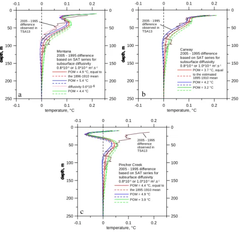
in temperature-depth are largely explained by the assumed SAT-POM forcing model. The TSA13 well #1 T-z transients can be explained by synthetic model based on the nearby SAT time series. The measured differences between the logs over the re-logging interval (2005–1995) are shown in Fig. 4 for the TSA13 Well #1 log located at Aden, in southern Alberta. The synthetic differences calculated from POM-SAT until

15

2005 minus POM-SAT until 1995 was done using SAT data from northern Montana (Fig. 4a), Carway (Fig. 4b), and Pincher Creek (Fig. 4c).

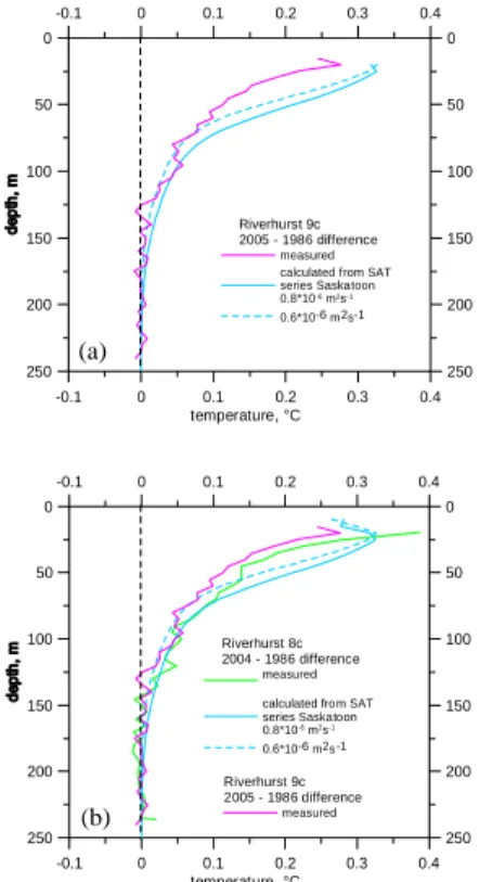
Figure 5a shows the differences between the logs over the re-logging interval for well T9C. The synthetic difference based on the SAT time series from the Saskatoon SAT station for the same time interval synthetic differences are shown for two diffusivity

20

values (0.6 and 0.8×10−6m2s−1) which cover the range of uncertainty in the estimate of the diffusivity for the clastic sediments. We also compare repeated logs for the T8C well and the T9C well (#8) which is located approximately 10 km from the T9C well the T8C well shows slightly greater warming between 1986 and 2004 than well T9C (by some 0.02◦C) (Fig. 5b) well T9C logs were taken at slightly different times (1986–

25

2005) both wells are located in southern Saskatchewan and the averaged synthetic difference was based on 1986–2004.5. The above experiment shows that the observed changes between repeated T-z logs and changes calculated from the model of SAT forcing and assumed POM compare well within the 0.03◦C error of temperature-depth

(11)

CPD

Full Screen / Esc

EGU

measurement (thermistor calibrations are typically 0.01◦C). For two wells, Gull Lake (#11 located close to a lake) and Sundrea (#12 located in the high recharge area of the Foothills), the simulated differences overestimate measured differences indicating that factors other than surface temperature change can influence the subsurface thermal regime. Twenty wells show warming in the initial logging and re-logging interval as

5

predicted from SAT-POM models. The average differences between measured and synthetic transients of T-z in the upper 100 m are smaller than 0.05◦C for nineteen wells.

4.1 Analysis of snow cover

Snow cover records from three stations in the southern Canadian Prairies are analyzed

10

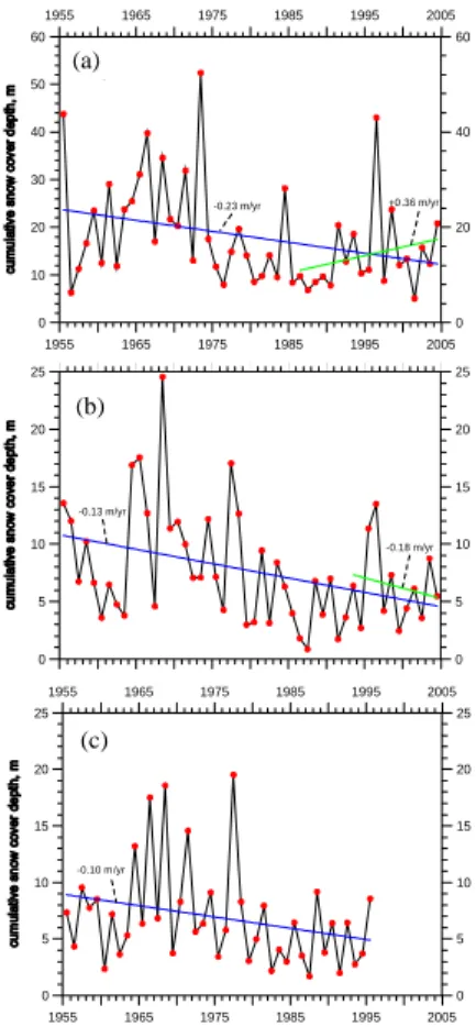
in conjunction with the period of well re-logging to provide more insight into the effects of snow cover on GST. Figure 6 shows the annual cumulative snow cover depth (from July to the next June) for three stations in the southern Prairies, Saskatoon Fig. 6a, Medicine Hat Fig. 6b, and Lethbridge Fig. 6c (Fig. 1 and Table 2). Variations of SAT-GST offset due to variations in the insulating properties of snow and variations in soil

15

moisture can be an important factor. According to Todhunter and Popham (2005), a snow cover index correlates very well with the thermal offset between SAT and GST. A downward trend in snow cover magnitude may provide some of the explanation for the misfit of climate station SAT and GST records. If the snow cover is thinning over time, there should be less effective insulation of heat stored in the soil, and thus a

20

reduced thermal offset during winter. Heat stored in the soil during the warm season would be lost during the cold season. This would produce a cooling of GST relative to SAT and introduce a cooling misfit in the GST for that period of observation. The southern Canadian Prairie stations have experienced a decrease in snow cover over the last 50 years. However, for the interval coinciding with the re-logging period (the

25

last two decades), changes in the snow index are of small magnitude and vary between stations. There is still a good fit between synthetic T-z differences based on SAT-POM model and measured differences. This supports findings of Bartlett et al., (2005) who

(12)

CPD

Full Screen / Esc

EGU

applied a snow-ground thermal model to a combined US-Canada-Alaska snow data set covering 1950–2002 and found a decrease in the influence of snow on ground temperatures over central Canada, due mainly to increased average winter SAT. 4.2 Comparison with northern Great Plains

Comparisons are made with T-z profiles from the geographically adjacent northern

5

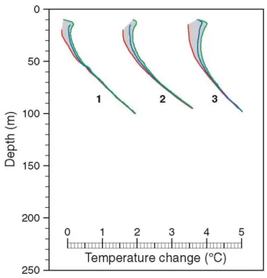
Great Plains of the USA (Gosnold et al., 1997). Table 1 in the Appendix provides well information on name, location, initial log and re-log years, terrain type, and GST warming calculated over the past century for all Canadian and USA wells used in this study. Figure 7 shows three examples of the well profiles in North Dakota that have been logged at least twice over a period of one or more decades. The scale allows for

10

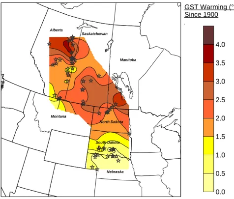
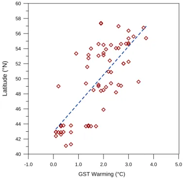
relative comparisons between logs. When combined with the Canadian data presented here, GST changes since 1900 can be shown spatially for the mid-western region of the continent. Figure 8 shows very large ground warming (1.5–4.0◦C) mainly in the southern Canadian Prairies and North Dakota where repeated logs analysed here also identify large warming over the past one to two decades. It is clearly evident that GST

15

has warmed over this period with a distinct south-to-north gradient to greater warming (Fig. 9). The measured GST warming over the past one to two decades can be largely explained by SAT forcing (Figs. 3 to 5). The warming over the previous century (Fig. 8) can also be explained by SAT forcing during the Industrial Age and post-Little Ice Age recovery (Majorowicz et al, 2006b).

20

5 Summary

The results presented here from repeated T-z measurements in boreholes in the south-ern Canadian Prairies show that SAT forcing is primarily responsible for the under-ground temperature changes diffusing with depth. It supports the borehole – tempera-ture paleoclimatology assumption that GST is systematically coupled with the surface

(13)

CPD

Full Screen / Esc

EGU

air temperature over the longer term (decades). The results also support the assump-tion that changes in GST diffuse mainly by conduction into the subsurface and impose a transient “climate” signal on the steady-state geothermal gradient. These assump-tions are limited to the sites where there is no hydrogeological disturbance. In the two cases where the differences between the synthetic and measured transients between

5

initial logging and repeated logging are higher than the error of measurement there is indication that factors other than SAT change can influence the subsurface thermal regime. An examination of cumulative snow cover depth from three Canadian Climate Network stations suggests there has been a decrease in the influence of snow cover on ground temperatures across the region during that re-logging interval. This is

co-10

incidental with increased winter SAT values. It is recommended that further repeated temperature logs from more northern locations in the Canadian Prairie provinces char-acterized by higher snowfalls be taken and compared to the SAT forcing as a borehole paleoclimatology testing method.

Acknowledgements. The first author would like to thank Environment Alberta and the

15

Saskatchewan Research Council for providing access to the well sites. Ed. J. Jaworski (S.R.C) and M. Magas (E.A. emeritus) assisted with guidance and removal of the piezometers for the time of logging of temperature. Support of NSF No. ATM – 0318384 (to W. Gosnold) and Environment is acknowledged.

References

20

Baker, D. G. and Ruschy, D. L.: The recent warming in eastern Minnesota shown by ground temperatures, Geophys. Res. Lett., 20, 371–374, 1993.

Bartlett, M. G., Chapman, D. S., and Harris, R. N.: Snow effects on North America ground tem-peratures, 1950–2002, J. Geophys. Res., 110, F03008 doi:10.1029/2005JF000293, 2005. Beach, R. D. W., Jones, F. W., and Majorowicz, J. A.: Heat flow and heat generation for the

25

Churchill of Western Canadian Sedimentary basin, Geothermics, 16, 1–16, 1987.

Carslaw, H. S. and Jaeger, J. C.: Conduction of Heat in Solids, Oxford Univ. Press, New York, 386 pp.,1959.

(14)

CPD

Full Screen / Esc

EGU

Ferguson, G. and Woodbury, A. D.: The effect of climatic variability on estimates of recharge derived from temperature data ground water, Ground Water Res., 43, 837–842, 2005. Gosnold, W. D., Todhunter, P. E., and Schmidt, W.: The borehole temperature record of climate

warming in the mid-continent of north America, Global Planet. Change, 15, 33–45, 1997. Gosnold, W., A., Dong, U., and Popham, J.: A test of borehole climatology, AGU Fall Meeting

5

abstract, AN:PP52A-0659, 2005.

Harris, R. N. and Gosnold, W. D.: Comparisons of borehole – depth profiles and and surface air temperatures in the northern plains of the USA Geophys. J. Int., 138, 541–548, 1999. Jessop, A. M.: Thermal Geophysics Developments in Solid Earth, Geophys., 17, Elsevier, 306

p., 1990.

10

Lewis, T.: The effect of deforestation on ground surface temperatures, Global Planet. Change, 18, 1–13, 1998.

Lewis, T. and Skinner, W.: Inferring climate change from underground temperatures: Apparent climatic stability and apparent climatic warming, Earth Interactions, 7, paper No. 9, 1–9, 2003.

15

Lachenbruch, A. H.: Permafrost, The active layer and changing climate, US Geol. Surv. Open-File Report 94-694 Menlo Park, CA, 1994, 43 pp., 1994.

Majorowicz, J. A. and Skinner, W. R.: Potential causes of differences between ground and sur-face air temperature warming across different ecozones in Alberta, Canada, Global Planet. Change, 15, 79–91, 1997.

20

Majorowicz, J. A. and Safanda, J.: Measured versus simulated transients of temperature logs, J. Geophys. Eng., 4, 291–298, 2005.

Majorowicz, J. A., Grasby, S., Ferguson, G., Safanda, J., and Skinner, W. R.: Paleoclimatic reconstructions in western Canada from borehole temperature logs: surface air temperature forcing and groundwater flow, Clim. Past, 2, 1–10, 2006a.

25

Majorowicz, J. A., Safanda J., Harris, R., and Skinner, W. R.: Large ground surface temperature changes of the last three centuries inferred from borehole temperatures in the southern Canadian prairies-Saskatchewan, Global Planet. Change, 20, 227–241, 1999.

Mann, M. E, and Schmidt, G. A.: Ground vs. Surface Air Temperature Trends: Implications for Borehole Surface Temperature Reconstructions, Geophys. Res. Lett., 30(12), 1607,

30

doi:10.1029/2003GL017170, 2003.

Mekis, E. and Hogg, W. D.: Rehabilitation and analysis of Canadian daily precipitation time series, Atmos.-Ocean, 37(1), 53–85, 1999.

(15)

CPD

Full Screen / Esc

EGU

Reiter, M.: Possible ambiguities in subsurface temperature logs – Consideration of ground – water flow and ground surface temperature change, Pure Appl. Geophys., 162, 343–353, 2005.

Shen, P, Yu and Beck, A. E.: Least squares inversion of borehole temperature measurements in functional space, J. Geophys. Res., 96, 19 965–19 979, 1991.

5

Schmidt, W. L., Gosnold, W. D., and Enz, J. W.: A decade of air-ground temperature exchange from Fargo North Dakota, Global Planet. Change, 29, 311–325, 2001.

Skinner, W. R. and Majorowicz, J. A.: Regional climatic warming and associated twentieth century land-cover changes in north-western North America, Clim. Res., 12, 39–52, 1999. Stieglitz, M., Romanovsky, V. E. and Osterkamp, T. E.: The role of snow cover in the warming

10

of arctic permafrost, Geophys. Res. Lett., 30, 1721, doi:10,1029/2003GL017337, 2003. Todhunter, P. E. and Popham, J. L.: Relationship Between Snow Cover and Thermal Offset

of Soil and Air Temperatures in the Great Plains of the United States, AGU Fall Abstracts, 2005.

Vincent, L. and Gullett, D. W.: Canadian historical and homogeneous temperature datasets for

15

climate change analyses, Int. J. Clim., 19, 1375–1388, 1999.

Zhang, X., Vincent, L. A., Hogg, D. W., and Niitsoo, A.: Temperature and precipitation trends in Canada during the 20th century, Atmos.-Ocean, 38, 395–429, 2000.

(16)

CPD

Full Screen / Esc

EGU

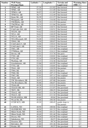
Table 1. Information on name, location, initial log and re-log years, and terrain type for 24 well

temperature logs in the southern Canadian Prairies.

Number Well Name Latitude (◦) Longitude (◦) Log Years Terrain 1 TSA13 49.08 111.33 1995, 2005 Grass 2 T967 52.01 107.11 1996, 2004 Grass 3 T964 52.26 105.52 1996, 2004 Grass 4 T965 53.06 103.95 1996, 2004 Grass 5 Sion 53.91 114.10 1992, 2004 Farmland 6 Devon 53.42 113.76 1992, 2004 Grass 7 Barhead 54.04 114.39 1992, 2004 Grass 8 T8c 50.88 106.87 1986, 2004 Grass 9 Warburg 53.13 114.36 1991, 2004 Grass 10 TPR2 55.61 116.68 1993, 2004 Forest 11 Gull Lake 52.63 114.05 1991, 2004 Farmland 12 Sundre 51.83 114.65 1991, 2004 Farmland 13 Olds 51.77 113.97 1991, 2004 Farmland 14 T9C 50.95 106.99 1986, 2005 Grass 15 TSA1 52.41 110.59 1995, 2005 Grass 16 TSA2 51.79 110.50 1995, 2005 Grass 17 TSA3 51.57 110.47 1993, 2005 Grass 18 TSA5 49.47 110.96 1993, 2005 Grass 19 TSA6 49.38 112.20 1993, 2005 Grass 20 TSA8 49.10 110.25 1995, 2005 Grass 21 TSA9 49.99 110.46 1995, 2005 Grass 22 TSA10 49.17 111.08 1995, 2005 Grass 23 TSA11 49.03 112.84 1995, 2005 Grass 24 TSA12 49.17 111.08 1995, 2005 GRASS

(17)

CPD

Full Screen / Esc

EGU

Table 2. Information on name, location, and element(s) used for six climate stations in the

study area.

Number Climate Station Latitude (◦) Longitude (◦) Climate Data A Pincher Creek 49.40 114.03 Air Temperature B Carway 49.00 113.37 Air Temperature C Saskatoon 52.12 106.65 Air Temperature

Snow cover D Medicine Hat 50.02 110.72 Snow cover E Lethbridge 49.70 112.85 Snow cover F Montana 7 station average Air Temperature

(18)

CPD

Full Screen / Esc

EGU

Number Well Name, Province/State

Latitude (°) Longitude (°) Terrain and Land Cover Warming Since 1900 (°C) 1 TFM2, AB 57.39 -111.82 flat forested 1.9 2 TFM1, AB 57.33 -111.69 flat forested 1.9 3 TFM14, AB 56.97 -111.85 flat forested 2.6 4 TFM15A, AB 56.77 -112.49 flat forested 3.6 5 Stony Mt., AB 56.39 -111.27 flat forested 3.0 6 Winagami, AB 55.61 -116.68 flat forested 3.2 7 T963Kirby, AB 55.39 -111.13 flat pasture 3.7 8 T962Wian, AB 55.35 -111.04 flat pasture 3.0 9 BP Triad, AB 54.74 -110.71 flat forested 3.0 10 Cold Lake 944, AB 54.65 -110.51 flat forested 2.9 11 TCL94, AB 54.62 -110.43 flat forested 2.7 12 TCL1, AB 54.61 -110.25 flat forested 1.8 13 TCL14, AB 54.57 -110.81 flat forested 3.0 14 TCL10Lessard, AB 54.48 -110.62 flat forested 2.3 15 TS941, SK 54.50 -109.87 flat forested 2.0 16 Cold Lake4-5, AB 54.06 -110.41 flat forested 2.6 17 Cold Lake3, AB 54.06 -110.41 flat forested 2.5 18 T961, AB 54.01 -113.18 flat cropland 1.5 19 T790Sion, AB 53.91 -114.11 flat cropland 2.1 20 Devon, AB 53.41 -113.76 flat grass 2.0 21 T765, AB 53.35 -110.01 flat cropland 0.9

22 T791,AB 53.16 -110.98 flat cropland 1.4 23 Warburg, AB 53.13 -114.36 flat,forested 2.0

24 Lloydminster, AB 53.06 -103.95 flat cropland 1.8 25 T754, AB 52.72 -110.85 flat cropland 1.4 26 TSA1, AB 52.41 -110.59 flat pasture 2.3 27 T964, SK 52.26 -105.52 flat grass 3.0 28 T966, SK 52.02 -107.12 flat cropland 2.8 29 T967, SK 52.01 -107.11 flat cropland 2.8 30 TSA3, AB 51.57 -110.48 flat prairie 1.4 31 T9C Rivenhurst, SK 50.95 -107.00 flat prairie 2.2 32 T8c Rivenhurst, SK 50.88 -106.87 flat prairie 2.3

33 TSA6,AB 49.38 -112.21 flat prairie 1.3 34 TSA10/10B, AB 49.18 -111.07 flat grassland 2.6

35 TKT1, SK 49.07 -106.25 flat grassland 2.7 36 TSA12, AB 49.02 -111.36 flat grassland 1.8 37 TSA13, AB 49.01 -111.32 flat grassland 0.2 38 WAWANESA, MB 49.60 -99.84 flat grassland 3.4 39 Wood Mt, SK 49.40 -106.40 flat prairie 2.3 40 CCDP-KT2, MB 49.20 -100.45 gentle slope to

flat pasture

1.8 41 LANDA, ND 48.90 -100.86 flat cropland 2.1 42 GLENBURN, ND 48.50 -101.33 flat cropland 2.0 43 Minot North, ND 48.50 -101.21 flat cropland 1.6 44 Minot South, ND 48.40 -101.46 flat cropland 1.9 45 Doyon, ND 48.20 -102.90 flat cropland 2.5 46 Sakakawea, ND 45.90 -96.97 flat grassland 2.0 47 Sisseton, SD 43.80 -99.74 flat grassland 0.3 48 Belvidere, SD 43.80 -101.26 flat grassland 0.7 49 Presho, SD 43.80 -99.57 flat grassland 0.4

Appendix Table 1.

15

Table A1. Temperature log information used for Fig. 8 warming since 1900 map for the

(19)

CPD

Full Screen / Esc

Printer-friendly Version Interactive Discussion EGU Figure 1. A B C Figure 1. D E 2 3 4 5 6 7 9 10 11 12₁₃ 15 14 17 18 19 20 21 23 22 8 16 24 1 F Alberta Saskatchewan Montana

Fig. 1. Twenty-four repeated well temperature logs locations, typical well site setting and the

remote sensing map of the Canadian Prairies (lighter colours show Prairie grasslands and farmland). Refer to Table 1 for more information on well sites. Also shown are the locations of the Canadian Historical Climate Network (HCN) and the USA Historical Climate Network (USHCN) sites used in the study. Refer to Table 2 for more information on the climate sites.

(20)

CPD

Full Screen / Esc

Printer-friendly Version Interactive Discussion EGU Well # 1 TSA13 Well # 14 T9C Well # 8 T8C (c) (b) (a) Figure 2. 2

Fig. 2. Examples from deep (>100 m) re-logged wells in the semi-arid southern Canadian

Prairies. Well #14(a) is a grassland site located in eastern Alberta near the Saskatchewan

border and was logged first in 1986 and again in 2005. Well #8(b) is also a grassland site and

located in southern Saskatchewan and was logged first in 1986 and again in 2004. Well #1

(c) is located in southern Alberta near the Montana border and was first logged in 1995 and

again in 2005. Note progressive warming with time in accordance with the basic assumption of conductive heat diffusion. All 24 sites temperature logs are shown Appendix Fig. 1.

(21)

CPD

Full Screen / Esc

Printer-friendly Version Interactive Discussion EGU 1890 1900 1910 1920 1930 1940 1950 1960 1970 1980 1990 2000 2010 1.0 2.0 3.0 4.0 5.0 6.0 7.0 8.0 9.0 A nn ua l S A T (° C)

Pre-Observational Mean (POM) 10-Year Running Average

(a) 1890 1900 1910 1920 1930 1940 1950 1960 1970 1980 1990 2000 2010 1.0 2.0 3.0 4.0 5.0 6.0 7.0 8.0 9.0 An n u al S A T (°C )

Pre-Observational Mean (POM) Ten-Year Running Average

(b) 1890 1900 1910 1920 1930 1940 1950 1960 1970 1980 1990 2000 2010 -1.0 0.0 1.0 2.0 3.0 4.0 5.0 6.0 7.0 8.0 9.0 An n u al S A T (°C )

(c) 1890 1900 1910 1920 1930 1940 1950 1960 1970 1980 1990 2000 2010 -3.0 -2.0 -1.0 0.0 1.0 2.0 3.0 4.0 5.0 6.0 7.0 A nn u a l S A T (° C)

(d)

Figure 3.

3

Fig. 3. Mean annual surface air temperatures (SAT) with their pre-observational means (POM)

and ten-year running averages for Pincher Creek(a), Alberta, northern Montana ensemble (b),

(22)

CPD

Full Screen / Esc

Printer-friendly Version Interactive Discussion EGU -0.1 0 0.1 0.2 temperature, °C 250 200 150 100 50 0 250 200 150 100 50 0 -0.1 0 0.1 0.2 Montana 2005 - 1995 difference based on SAT series for subsurface diffusivity 0.8*10- 6_{or 1.0*10}-6_m2_.s- 1 POM = 4.9 °C, equal to the 1896-1910 mean POM = 5.4 °C diffusivity 0.6*10-6 POM = 4.4 °C 2005 - 1995 difference observed in TSA13 -0.1 0 0.1 0.2 temperature, °C 250 200 150 100 50 0 250 200 150 100 50 0 -0.1 0 0.1 0.2 Carway 2005 - 1995 difference based on SAT series for subsurface diffusivity 0.8*10- 6_{or 1.0*10}-6_m2_.s- 1 POM = 3.7 °C, equal to the estimated 1895-1910 mean POM = 4.2 °C POM = 3.2 °C 2005 - 1995 difference observed in TSA13 -0.1 0 0.1 0.2 temperature, °C 250 200 150 100 50 0 250 200 150 100 50 0 -0.1 0 0.1 0.2 Pincher Creek 2005 - 1995 difference based on SAT series for subsurface diffusivity 0.8*10- 6_{or 1.0*10}- 6_m2_.s- 1 POM = 4.4 °C, equal to the 1895-1910 mean POM = 4.9 °C POM = 3.9 °C 2005 - 1995 difference observed in TSA13 a b c Figure 4.

Fig. 4. Comparison of the temperature difference between 1995 and 2005 with models based

on SAT forcing for TSA13 Well (#1) and northern Montana annual SAT ensemble(a), Carway

annual SAT(b), and Pincher Creek annual SAT (c), for a set of pre-observational means (POM

are given in the figures). Note good compatibility between observations and models considering uncertainties in POM assumption except for the Pincher Creek series (see Fig. 3a) where there has been local cooling close to the Rocky Mountain foothills over the past decade.

(23)

CPD

Full Screen / Esc

Printer-friendly Version Interactive Discussion EGU -0.1 0 0.1 0.2 0.3 0.4 temperature, °C 250 200 150 100 50 0 250 200 150 100 50 0 -0.1 0 0.1 0.2 0.3 0.4 Riverhurst 9c 2005 - 1986 difference measured calculated from SAT series Saskatoon 0.8*10-6 m2s-1 0.6*10-6 m2s-1 -0.1 0 0.1 0.2 0.3 0.4 temperature, °C 250 200 150 100 50 0 250 200 150 100 50 0 -0.1 0 0.1 0.2 0.3 0.4 Riverhurst 8c 2004 - 1986 difference measured calculated from SAT series Saskatoon 0.8*10-6 m2s-1 0.6*10-6 m2s-1 Riverhurst 9c 2005 - 1986 difference measured (a) (b) Figure 5. 5

Fig. 5. Comparison of the temperature difference between 1986 and 2005 for the Riverhurst,

Saskatchewan T9C well (#14)(a) with the synthetic temperature difference for the same time

period calculated from SAT forcing in Saskatoon SAT HCN station, and comparison of the temperature difference between 1986 and 2004 for the Riverhurst, Saskatchewan T8C well (#14)(b) with the synthetic temperature difference for the same time period calculated from

SAT forcing in Saskatoon SAT HCN station calculated for the 1986–2004.5 period. Calculations are done for two sets of diffusivity values (0.6 and 0.8×10−6m2s−1). The T8C well site warmed slightly more than T9C well site (0.02◦C) over similar time difference (18 years and 19 years respectively).

(24)

CPD

Full Screen / Esc

Printer-friendly Version Interactive Discussion EGU 1955 1965 1975 1985 1995 2005 0 10 20 30 40 50 60 0 20 40 60 1955 1965 1975 1985 1995 2005 -0.23 m/yr +0.36 m/yr a 0 5 10 15 20 25 0 5 10 15 20 25 -0.13 m/yr -0.18 m/yr b 1955 1965 1975 1985 1995 2005 time, year 0 5 10 15 20 25 1955 1965 1975 1985 1995 2005 0 5 10 15 20 25 -0.10 m/yr c (a) (b) (c) Figure 6. 6

Fig. 6. Cumulative annual snow cover for three long Canadian Historical Climate Network

sta-tions in the southern Canadian Prairies, Saskatoon, Saskatchewan(a), Medicine Hat Alberta (b), and Lethbridge, Alberta (c).

(25)

CPD

Full Screen / Esc

EGU

Figure 7.

Fig. 7. Repeated logs for three North Dakota, USA wells, Landa (1), Minot (2) and Glenburn

(3) (Gosnold et al., 2005). See Appendix Table 1 for the locations and well site information.

(26)

CPD

Full Screen / Esc

Printer-friendly Version Interactive Discussion EGU 0.0 0.5 1.0 1.5 2.0 2.5 3.0 3.5 4.0 GST Warming (°C) Since 1900 Alberta Saskatchewan Manitoba Montana North Dakota South Dakota Nebraska Figure 8.

Fig. 8. Ground warming (◦C) since 1900 derived from numerous well logs taken over last 2 decades (initial logs plus repeated logs) in the Canadian Prairies (J. A. Majorowicz logs – Environment Canada projects) and by the University of North Dakota. Refer to Appendix Table 1 for information on well sites used in contour map.

(27)

CPD

Full Screen / Esc

Printer-friendly Version Interactive Discussion EGU -1.0 0.0 1.0 2.0 3.0 4.0 5.0 GST Warming (°C) 40 42 44 46 48 50 52 54 56 58 60 Lat it ude (°N) Figure 9.

Fig. 9. GST warming since 1900 by latitude from North American well temperature logs listed

in Appendix Table 1.

(28)