HAL Id: hal-01457992
https://hal.sorbonne-universite.fr/hal-01457992
Submitted on 6 Feb 2017
HAL is a multi-disciplinary open access
archive for the deposit and dissemination of sci-entific research documents, whether they are pub-lished or not. The documents may come from teaching and research institutions in France or abroad, or from public or private research centers.
L’archive ouverte pluridisciplinaire HAL, est destinée au dépôt et à la diffusion de documents scientifiques de niveau recherche, publiés ou non, émanant des établissements d’enseignement et de recherche français ou étrangers, des laboratoires publics ou privés.
Large-Eddy Simulations of Dust Devils and Convective
Vortices
Aymeric Spiga, Erika Barth, Zhaolin Gu, Fabian Hoffmann, Junshi Ito,
Bradley Jemmett-Smith, Martina Klose, Seiya Nishizawa, Siegfried Raasch,
Scot Rafkin, et al.
To cite this version:
Aymeric Spiga, Erika Barth, Zhaolin Gu, Fabian Hoffmann, Junshi Ito, et al.. Large-Eddy Simulations of Dust Devils and Convective Vortices. Space Science Reviews, Springer Verlag, 2016, 203, pp.245 -275. �10.1007/s11214-016-0284-x�. �hal-01457992�
Large-Eddy Simulations
of dust devils and convective vortices
Aymeric Spiga
∗1, Erika Barth
2, Zhaolin Gu
3, Fabian Hoffmann
4, Junshi Ito
5,
Bradley Jemmett-Smith
6, Martina Klose
7, Seiya Nishizawa
8, Siegfried Raasch
9,
Scot Rafkin
10, Tetsuya Takemi
11, Daniel Tyler
12, and Wei Wei
131
Laboratoire de M´et´eorologie Dynamique, UMR CNRS 8539, Institut Pierre-Simon Laplace, Sorbonne Universit´es, UPMC Univ Paris 06, Paris, France
2SouthWest Research Institute, Boulder (Colorado), USA 3Xi’an Jiaotong University, Xi’an, China
4Institute of Meteorology and Climatology, Leibniz Universit¨at Hannover, Hannover, Germany 5Meteorological Research Institute, Ibaraki, Japan
6Institute of Climate and Atmospheric Science, University of Leeds, Leeds, United Kingdom 7Institute for Geophysics and Meteorology, University of Cologne, Cologne, Germany
8RIKEN Advanced Institute for Computational Science, Kobe, Japan
9Institute of Meteorology and Climatology, Leibniz Universit¨at Hannover, Hannover, Germany 10SouthWest Research Institute, Boulder (Colorado), USA
11Disaster Prevention Research Institute, Kyoto University, Kyoto, Japan 12Oregon State University, Corvallis (Oregon), USA
13Wuhan University of Technology, Wuhan, China
Published: Space Science Reviews, 203:245-275, 2016
Abstract
In this review, we address the use of numerical computations called Large-Eddy Simulations (LES) to study dust devils, and the more general class of atmospheric phenomena they belong to (convec-tive vortices). We describe the main elements of the LES methodology. We review the properties, statistics, and variability of dust devils and convective vortices resolved by LES in both terrestrial and Martian environments. The current challenges faced by modelers using LES for dust devils are also discussed in detail.
1
Introduction
In this chapter, we describe dust devils as events worthy of interest in atmospheric fluid dynamics. A dust devil is a particular case of a more general dynamical phenomenon, the convective vortex, occurring in the Planetary Boundary Layer (PBL), the part of the atmosphere directly influenced by the presence of the planetary surface. Convective vortices form during daytime hours when the warm surface causes strong convective instabilities to occur in the PBL, giving rise to the Convective Boundary Layer (CBL). A dust devil appears when one convective vortex has the ability (for a variety of reasons, one being the availability of dust particles at the surface) to lift and advect dust in its swirling circulation structure. A given area might be prone to the occurrence of convective vortices, but devoid of visible dust devils.
Herein we specifically describe the numerical modeling of dust devils by turbulence-resolving simulations called Large-Eddy Simulations (LES). In LES, the equations of motion for the atmo-spheric fluid are integrated on a gridded mesh with a typical spacing of tens of meters or less in order to resolve the larger turbulent eddies that are responsible for most of the energy transport within the CBL. Thus, LES are capable of resolving dust devils, which have diameters smaller than 1 km (see Murphy et al. (2016), Fenton et al. (2016), and Lorenz and Jackson (2016) in this issue), in contrast to simulations carried out by either Global Climate Models (GCM, in which mesh spacing is a couple hundreds of kilometers) or Regional Climate Models (RCM, in which mesh spacing is typically several kilometers) (Figure 1). Furthermore, in LES, convective vortices possibly leading to dust devils are explicitly resolved. This is in contrast to other modeling work described in this special issue, where either dust transport by dust devils is predicted without resolving the individual structure (see Rafkin et al. (2016) in this issue), or pre-existing vortical structures are prescribed (see Kurgansky et al. (2016) in this issue). It shall be emphasized, how-ever, that the smallest-diameter dust devils observed on both the Earth and Mars (a couple meters accross) are still challenging to resolve with LES.
An important aspect to bear in mind in this chapter is that the occurrence of convective vortices is inseparable from the growth and mature stage of the CBL in daytime. Hence, reproducing convective vortices is only one of the overarching goals of LES which, in a broader sense, aim at exploring the whole range of atmospheric phenomena associated with the CBL growth: convective cells, plumes, vortices, and the resulting mixing of heat and momentum. In addition to CBL dynamics, LES offer interesting modeling perspectives for the stable and neutral PBL.
In this chapter, we review what LES brought to the study of dust devils and convective vortices. LES have been instrumental in broadening the knowledge of the properties, evolution, and statistics of dust devils. The LES modeling approach is highly complementary to measurements (see Murphy et al. (2016) and Fenton et al. (2016) in this issue) to study dust devils, since all properties of modeled vortices (wind speed, temperature, pressure, stability), as well as local environmental conditions, are accessible with LES.
We discuss LES performed in the context of both the Earth and Mars. Comparing the two environments gives insight into the mechanisms and characteristics of convective vortices in general, with Mars’ strong near-surface gradients of temperature making the Red Planet an interesting extreme counterpart to the Earth for CBL studies.
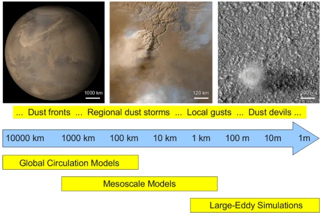
Figure 1: Typical dust lifting events (top images + yellow strip), relevant spatial scales (middle blue arrow) and meteorological models suitable for their analysis (bottom yellow strips). Left: Dust front observed through Mars Orbiter Camera (MOC) imagery. Middle: Dust regional storm observed with MARs Color Imager (MARCI). Right: Dust devil observed with HIgh Resolution Imaging Science Experiment (HIRISE). Note that: 1. the lower bound of the GCM mesh spacing continues to decrease as computational capability and modeling techniques improve; 2. mesoscale modeling and (turbulence-resolving) Large-Eddy Simulations can be often carried out with the same non-hydrostatic dynamical core; 3. the horizontal scale is neither unique nor the best possible choice by which to classify dust events: obviously meteorological origin (fronts, deep convection, turbulence, . . . ) allows for a better understanding, although this criterion may be less straightforward for a broader audience to understand. Figure published in Spiga and Lewis (2010), used with permission.
2
LES methodology
2.1
Dynamical integrations
LES consist of four-dimensional (horizontal+vertical+temporal) numerical integrations of atmo-spheric fluid dynamics equations, usually the fully compressible, non-hydrostatic Navier-Stokes equations. While the vast majority of GCM simulations are performed under the approximation of hydrostatic balance between gravity and pressure forces in the vertical, such an approximation is not appropriate in LES because vertical wind accelerations in CBL turbulent structures might become comparable to the acceleration due to gravity. For hydrodynamical integrations, Martian LES are based on similar solvers as terrestrial LES: e.g., for their Martian studies, Rafkin et al. (2001) (see Section 4.1) used the RAMS terrestrial model (Pielke et al., 1992), and Spiga and Forget (2009) used the WRF model (Moeng et al., 2007; Skamarock and Klemp, 2008), also used by Klose and Shao (2013) to simulate terrestrial CBL vortices (see Section 3 and Tables 1 and 2). A remaining cornerstone for the proper simulation of dust devils, even in high-resolution LES, is the application of suitable numerical schemes. The numerical approximations used by the schemes cause characteristic numerical errors due to their specific construction (e. g., Durran, 2010, Chapter 3). Numerical diffusion is usually caused by schemes of odd order of accuracy, whereas numerical dispersion is caused by schemes of even order. Numerical dispersion is triggered by strong gradients of the advected quantities, which typically exist in the center of dust devils. The resulting wiggles are cumbersome for the development and evolution of dust devils. By comparing a standard advection scheme to a scheme which is especially designed to avoid these errors, Weißm¨uller et al. (2016) showed that the average central pressure drop intensity increases by 8 % if the latter scheme is used.
Generally speaking, every LES model is capable of carrying out dynamical integrations at very high horizontal resolution. However, the increasing number of simulated grid points is accompanied by increasing demands on the model’s high-performance computing capabilities, such as its efficient parallelization, which is necessary to distribute the simulation on up to thousands of computing nodes, and the optimized handling of data, simply because a higher number of grid points produces more data, which has to be processed and analyzed.
2.2
Domain extent
LES integrations are carried out on a limited-area horizontal domain. LES are often qualified as idealized simulations, for this limited domain is associated with uniform surface conditions (e.g. topography, albedo, thermal inertia, solar forcing, roughness) and doubly periodic boundary con-ditions, effectively resulting in a simulation of an infinite flat plane. It is an open question whether this is a valid approach in the strictest sense to LES either for the Earth or for Mars: the approx-imation is probably satisfactory for a large enough flat area, but cannot properly address items such as the formation of dust devils near slightly larger-scale topographical or albedo contrasts (Renno et al., 2004). Furthermore, periodic lateral boundaries prevent LES from accounting for any gradients in regional or large-scale circulations.
the LES domain must be both deep enough and wide enough to contain at least several of the largest polygonal cells that develop in the CBL (an aspect ratio of three, width/depth, is minimally sufficient as is discussed in Mason, 1989). Otherwise, a single (or, in the worst-case scenario, half a) polygonal cell might be aliased by the periodic boundary conditions, leading to unrealistic results. For Mars, following the deeper CBL mixing layer (up to 10 km deep vs. a few kilometers deep on the Earth, see Spiga, 2011, and references therein), horizontal convective cells are larger in both dimensions by at least a factor of two, whereas the actual size of dust devils can be very similar to those on the Earth. This leads to a very large computational burden when performing LES on Mars, at least an order of magnitude larger cost when taking into consideration the lower timestep necessary to resolve the more vigorous vertical velocities encountered on Mars compared to the Earth. The state-of-the-art LES for the Martian CBL has not yet surpassed this obstacle, an aspect that should be kept in mind when further discussing convective vortices and dust devils in Martian LES.
This issue on the size of the LES domain, quite specific to the Martian environment, is also encountered in terrestrial LES when computationally demanding high-resolution LES are carried out. A proper representation of the fundamental boundary layer dynamics, i. e., the cellular pattern of convection, is as important as the highest possible resolution for the successful simulation of dust devils (e. g., Raasch and Franke, 2011). Since the cells’ vertices are one of the main dust devils’ point of origin (see Section 3.2), dust-devil LES should not only feature a grid spacing in the order of meters for the successful simulation of the dust devil microstructure, but also a model domain adequate to well-represent larger-scale CBL dynamics – generally multiple kilometers or more in all directions, depending on the location and time-of-day.
2.3
Treatment of sub-grid scale processes
Turbulence is the dominant mechanism of vertical atmospheric mixing. As mentioned in the introduction, the mesh spacing typically used for the LES horizontal grid is from a few tens of meters to a few meters, i.e. suitable to resolve the largest turbulent eddies responsible for about 80%-90% of the energy transport in the CBL (hence the name LES, cf. Lilly, 1962; Sullivan and Patton, 2011). Contrary to what is done in GCMs and RCMs, LES resolve the large turbulent eddies, i.e. convective plumes and vortices. Hence the mixing of heat and momentum they produce does not need to be parameterized. In other words, LES allow for a more fundamental study of the CBL. Still, LES lack the mixing produced by the unresolved small-scale eddies. This includes any turbulent phenomena at smaller scales than the adopted LES grid spacing, part of which can be the smallest convective vortices (and related dust devils). The treatment for this small-scale mixing in LES can be achieved by computing the eddy diffusivity (i.e., turbulent mixing coefficients) from either the local velocity and temperature gradients (Smagorinsky, 1963), or subgrid Turbulent Kinetic Energy (TKE) prognosed from a high-order closure equation Deardorff (1972). The latter strategy is usually adopted in LES (see e.g. Moeng et al., 2007), while the former is more typical of GCM and RCM (though it is also used in LES, e.g. Kanak et al., 2000). The treatment of subgrid-scale mixing in Martian LES is similar to terrestrial LES, although the latest developments on TKE-based schemes for terrestrial LES Mirocha et al. (2010) are yet to be considered for use in Martian LES.
The Surface Layer (SL) is the part of the PBL immmediately adjacent to the surface. The SL thickness is several meters to tens of meters on Earth (and on Mars, although this is yet to be confirmed by direct measurements Petrosyan et al., 2011). The whole SL thickness is thus usually enclosed in the 1−2 lowermost atmospheric levels in LES. Furthermore, turbulent motions in the SL develop at lower spatial and temporal scales than what is achievable by LES. Hence, SL processes are in need to be parameterized in LES, as is the case in GCMs and RCMs. This basically means developing a simple model for the surface-atmosphere transfer of heat, momentum, and tracers. For instance, the quantity related to heat transfer from the surface to the atmosphere via the SL is the sensible heat flux Hs. The simplest SL parameterization for Hs is a bulk parameterization
in which Hs is simply proportional to the specific heat capacity of the surface, the atmospheric
density, the wind stress exerted by the atmosphere on the surface, and the surface-atmosphere temperature contrast. Under simplifying assumptions, the last two quantities can be calculated respectively from the wind and temperature predicted at the lowermost atmospheric model layer. More accurate SL parameterizations account for the variation of the surface-atmosphere transfer coefficient (both for heat and momentum) with nighttime stable vs. daytime unstable conditions (e.g. Haberle et al., 1993).
2.4
Coupling dynamical integrations with physical processes
Within the CBL, the mixing of heat through turbulent motions (adiabatic heat transfer) typi-cally dominates the atmospheric thermal structure. Diabatic processes (such as radiative transfer, molecular conduction with the surface, and volatile phase change) also modulate the static stability profile within and above the CBL, hence the intensity and vertical extent of convective motions. The phase change of volatiles is often insignificant for the arid areas/seasons that exhibit dust devil activity. Radiative forcing includes the absorption of incoming solar flux (by aerosols, i.e. dust particles in deserts) and the absorption/re-emission of infrared flux outgoing from the surface (by greenhouse gases and aerosols). Accounting for radiative forcing in LES may be separated into three categories, which illustrate major differences in the predominance of radiative processes between Mars and the Earth.
• Category 1 If the radiative heating rates can be neglected, typically in hour-long terrestrial LES aimed at investigating a particular phenomenon, no radiative processes are included, and a fixed sensible heat flux value is imposed at the bottom of the atmosphere. For in-stance, Klose and Shao (2013) investigated CBL dynamical stuctures leading to particle lifting through 90-minute long LES runs using 200 × 200 horizontal grid points with 10 m mesh spacing. The combination of both idealized character and short duration for this LES setup reflects the limitations imposed by the timestep of 0.05 seconds; neither performing a longer run nor including radiative processes would have been crucial for the scientific objec-tives of Klose and Shao (2013) (other examples are e.g. Zhao et al., 2004; Kanak, 2006). • Category 2 If radiative heating cannot be neglected, but radiative timescales are larger than
typical convective timescales, precalculated (offline) time-varying radiative heating rates are employed. This setting is typically employed for daytime terrestrial LES – although Category 1 LES also yields correct results (to first order) in this configuration. Category 2 LES appears
to yield acceptable results for Mars (Sorbjan, 2007; Gheynani and Taylor, 2011), although this remains to be tested more thoroughly.
• Category 3 If radiative heating is significant, and radiative timescales are smaller than typ-ical convective timescales, the dynamtyp-ical integrations must be coupled with time-marching (online) radiative computations – usually associated with a ground model to account for subsurface heat transfers. This setting is typically employed for Martian LES because the thin CO2 atmosphere loaded with dust on Mars leads to both fast radiative timescales and
a predominance of the divergence of infrared radiative flux over sensible heat flux within near-surface atmospheric levels (Haberle et al., 1993; S¨avijarvi, 1999; Spiga et al., 2010). Category 3 LES also emerged recently for the Earth, to study areas particularly prone to the radiative influence of airborne dust, with a model coupling radiation and land-surface schemes (Shao et al., 2013).
Whether or not such modeling assumptions change the predictions for convective vortices in LES remains an open question, both for the Earth and for Mars.
Initializing LES is usually handled with a prescription of the same initial temperature and background wind profiles at every horizontal grid point. Temperature profiles are usually extracted from GCM or RCM simulations; on terrestrial LES, atmospheric soundings are also being used as initial conditions. Prescribing at all vertical levels the exact same temperature for the entire horizontal domain imparts a symmetry that does not exist in reality – small-scale, low-amplitude temperature fluctuations are ever-present in a real atmosphere. Random (noise) temperature perturbations of about 0.1 K are therefore added to the initial temperature field to break the horizontal symmetry of this initial field, and help trigger convective motions. Often LES are run without prescribing a background wind profile, in what is called “free convection” LES. Somewhat more realistic scenarios, where the horizontal wind is forced by the geostrophic wind derived from a mesoscale model, have been performed for Mars (e.g., Tyler et al., 2008). Such a strategy was primarily employed to account for the strong diurnal cycle of synoptic and regional winds on Mars, driven by thermal tides and slope flow. In terrestrial LES, experiments which include the Coriolis force to simulate the effect of background wind rotation were performed by Ito et al. (2011).
It is commonly assumed in the various published studies that the first half-hour / hour of a simulation should be considered as a spin-up from the initial state to the resolved LES state. Except for the finest resolutions, which clearly limit the total duration of the LES integrations, or LES driven by the same forcing throughout the simulation, most LES are usually started very early in the morning (local time 6 to 8 AM) to allow for this spin-up to occur before the CBL starts to develop and grow in earnest as the sun rises higher.
2.5
Dust particles
Thus far, the vast majority of LES studies have been used to study convective vortices rather than true dust devils. In other words, the emphasis has been put on the dynamics and statistics of CBL vortices, with neither dust lifting nor dust transport processes included to form realistic dust devils. LES for Mars typically use a uniform background dust opacity; on the Earth, LES are often conducted without explicit dust treatment.
Progress has been made recently by including a representation for the full dust cycle (i.e. emission, transport, and deposition of dust particles) into terrestrial and Martian LES (Klose and Shao, 2013). The first efforts towards this goal date back to the terrestrial LES study of Zhao et al. (2004), in which sand particles are injected into their dust-devil scale simulation to study dust transport and deposition, although no explicit formulation for dust entrainment is used. The first LES investigation to include a saltation bombardment scheme is the Martian study by Michaels (2006). The author uses the LES friction velocities to calculate bulk fluxes of dust and sand (partitioned according to a predefined particle-size distribution), that are then removed from the ground, transported within the modeled atmosphere, and ultimately fall back to the ground. The focus of Michaels (2006) was on the formation of dust devil tracks though – and not on the dust emission fluxes generated by dust devils. This was more the focus of Ito et al. (2010a), who included dust lifting in their LES model by using the empirical formulation of Loosmore and Hunt (2000). According to this formulation, dust emission is proportional to friction velocity, u∗. However,
Loosmore and Hunt (2000) have obtained their formulation for background dust lifting in the absence of saltation and without focus on convective turbulence. The fluxes obtained by Ito et al. (2010a) in their simulation of the convective boundary layer are thus relatively low. To overcome this limitation, Klose and Shao (2013) included a physics-based dust emission scheme (Klose and Shao, 2012) in their LES model and simulated dust emission due to convective turbulence (see Neakrase et al. (2016) in this issue). After further model developments and calibration against field measurements for dust emission, Klose et al. (2014) were the first to explicitly simulate size-resolved dust entrainment by dust devils.
This move towards more realistic prediction of the feedbacks between CBL dynamics and dust lifting – and thus the formation of spontaneous dust devils in LES – is still being more fully developed for both terrestrial and Martian LES. In the latter case, assessing the radiative effect of dust carried within a dust devil (as suggested by Fuerstenau, 2006) would be an interesting open question to address through LES. This would relate to a new Category 4 (see section 2.4) where radiative transfer and dynamical transport are fully coupled.
3
LES for the Earth
3.1
First LES studies for convective vortices
As pointed out by Kanak (2006), Mason (1989) may have been one of the first to present evidence of convective vortices in LES for the terrestrial CBL, but those were not the focus of his study, nor were they discussed. Experimental and computational efforts in the early 1990s allowed the gathering of robust evidence of spiraling updrafts in Rayleigh-B´enard convection (e.g. Cortese and Balachandar, 1993), but the applicability of this body of work to CBL convective vortices and dust devils was only considered after the first LES studies on this topic (Fiedler and Kanak, 2001).
It is generally accepted that the first work to report three-dimensional high-resolution LES capable of spontaneously generating convective vortices on scales similar to dust devils is Kanak et al. (2000), later complemented by Kanak (2005) (Figure 2). The importance of convective tilting of horizontal vorticity in dust devil formation is demonstrated by simulations that show
vortices forming within convergent branches of convective cells (and not only at cell vertices). The convective vortices modeled in LES agree well with field measurements (see Murphy et al. (2016) in this issue), showing similar velocity structure and diurnal behavior as actual dust devils (Table 1). However, some differences from observations were noted in the vortex intensity in terms of the central pressure deficit, where the simulated vortices are weaker than the observations: Kanak (2005) found that the central pressure drop deviated from measured values in Sinclair (1973) by nearly a factor of 5. This difference may be due to the effects of the spatial resolutions used in the simulations. Nevertheless, even a horizontal mesh spacing of 2 m in Kanak (2005), a significant increase from the resolution of 35 m in Kanak et al. (2000), did not improve the intensity of simulated dust devils because the diameters of the simulated vortices in Kanak (2005) were still larger than those observed (and thus insufficiently resolved). In spite of the deficiencies in LES pointed out in Kanak (2005), qualitative analyses on the dynamics and mechanisms of dust devils have been conducted in subsequent studies and have permitted the knowledge of those phenomena to progress.
Figure 2: Convective vortices in terrestrial LES. Horizontal cross-sections 2 m above the surface of velocity vectors from 2 m LES simulations after 1000 simulated seconds. Left: vectors at every fourth grid point over the total domain of 740 × 740 m2. Right: expanded vortex of interest on 80 × 80 grid points, with a vector plotted at every grid point. Figure published in Kanak (2005), used with permission.
3.2
Mechanisms for vortex formation in LES
Kanak (2006) emphasizes that LES demonstrate that no source of ambient angular momentum / wind shear is required to be imposed in order for vertical vortices to form: those occur even in LES devoid of background wind (cf. also Rafkin et al. (2016) in this issue). The mechanisms by which convective vortices and dust devils appear in LES are still being debated. Raasch and
Paper Dyn. dx Nx,y Z Nz w0 v0 P0 ζ core (m) (km) (m/s) (m/s) (Pa) (s−1) Kanak00 specific 35 86 2.1 48 0.15 5 18 0.1 Kanak05 specific 2 370 1.2 86 < 0.1 6 43 2.5 Ohno10a WRF 3 333 1.5 185 1.5 - 64 2 Ohno10b WRF 10 200 1.5 70 - - 70 0.8 Ito10 specific 50 90 3 60 4 6 40 0.3 Raasch11 PALM 2 2000 1.7 449 2 4 72 6.8 Ito13 specific 5 360 1.6 320 0.5 4.5 - 1.0
Table 1: Properties of modeled convective vortices in published LES studies in terrestrial conditions. Maximum values are reported, and shall be compared only to the order of magnitude level, given the differences in grid settings and prescribed background winds (for the latter point, cf. text for a more extended discussion). dx is the horizontal mesh spacing employed in LES, Nx,yis the number of grid points in the horizontal (x- and y-axis), Z is the altitude above the surface of the adopted model top, Nz is the number of grid points in the vertical (note that the vertical resolution changes with height, with higher resolution closer to the surface), [w0, v0] are respectively the updraft velocity and tangential velocity within a simulated convective vortex, [P0, ζ] are respectivey the pressure drop and the magnitude of vertical vorticity associated with the vortex.
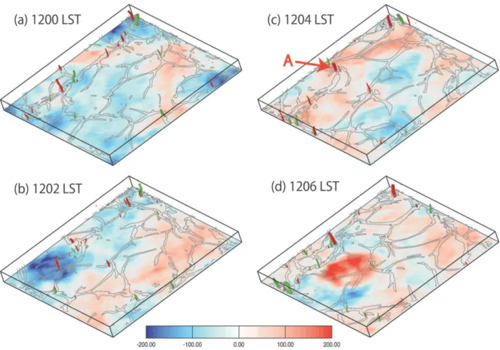
Franke (2011) studied the generation of dust devils by examining the vorticity budget, which has been directly derived from LES. They found that the vorticity of dust devils is mainly produced by twisting the vorticity generated by shear close to the surface from a horizontal to a vertical direction – a conclusion similar to the one reached by Kanak (2005) with coarser-resolution LES. In other words, those studies highlight the prominent role played by updrafts in CBL cells close to the surface. The LES study of Ito et al. (2013) indicated, however, that the origin of vorticity structures could also be traced back to downdrafts in CBL cells, and that the circulations can be originally generated by tilting of baroclinically generated horizontal vorticity within the CBL mixed layer, rather than closer to the surface (Figure 3). This apparent discrepancy between the two studies (Raasch and Franke, 2011; Ito et al., 2013) might simply reflect the variety of possible initial vorticity sources for the formation of dust devils in the CBL. At any event, Ohno and Takemi (2010a) demonstrated that, once formed, a vortex with a significant intensity will be further intensified through the merger with surrounding vortices (Figure 4).
3.3
Influence of environmental conditions on convective vortices
How environmental conditions impact the properties of convective vortices is addressed in detail in Rafkin et al. (2016) in this issue. Here we review the main results obtained through LES on this topic. Takemi (2008) examined the influence of atmospheric stability on the development of daytime CBL and vertical dust transport by conducting high-resolution RCM simulations (with an horizontal resolution of 100 m, which makes it coarse-resolution LES) and found that an early morning stable stratification strongly regulates the temporal evolution and the vertical growth of convection and therefore the amount of dust emission and transport. Ohno and Takemi (2010b) investigated the effects of background wind speed on the generation of vortices and found that
Figure 3: The origin of convective vortices resolved by terrestrial LES. Time series of vertical vorticity iso-surfaces of 0.25 (red) and -0.25 s−1 (green) from (a) 1200 to (d) 1206 local time, at 2-min intervals. The lower domain at heights < 100 m is displayed. Circulation, calculated only for downdraft regions within a horizontal circle of radius 300 m at each grid point at z = 2.5 m, is shown by color shading (m2 s−1). Regions where vertical velocities are > 0.1 m s−1 at the lowest model level are shown by gray isolines. The horizontal domain shown is 1.8 km accross. Figure published in Ito et al. (2013), used with permission.
Figure 4: Merging of two convective vortices simulated by terrestrial LES. Horizontal sections of wind vectors, vertical velocity (shaded) and vertical vorticity (contoured at 0.3 s−1 interval from 0.15 s−1) at the 1.5 m height. Figure published in Ohno and Takemi (2010a), used with permission.
vortices are generated most preferably in medium-wind conditions in terms of their number, in-tensity, and lifetime. Ohno and Takemi (2010b) also indicated that a stability condition controls the generation of dust devils, as was identified by Takemi (2008) and from field observations (see Murphy et al. (2016) in this issue).
Other LES modeling studies confirmed and complemented those findings. In the sensitivity experiment of Ito et al. (2010b), the strong vorticity extrema corresponding to convective vortices – and thus possible dust devils – are more frequent when both the background wind is weaker (as is also found by Ohno and Takemi, 2010b) and sensible heat flux is stronger. Those findings are consistent with observations (see Murphy et al. (2016) and Rafkin et al. (2016) in this issue). Ito et al. (2010b) compared experiments with nearly calm environmental wind (0.5 m s−1) and those with much stronger winds (5 − 15 m s−1). Other studies (e.g., Raasch and Franke, 2011) suggest that an intermediate, moderate background wind of a couple m s−1 is the most propitious condition for the formation of convective vortices.
3.4
Influence of horizontal resolution adopted in LES
Although relatively coarse-resolution LES (e.g. 50 m horizontal resolution in Ito et al., 2010b) are able to resolve the characteristic structure of dust devils at least qualitatively, there is still much room for improvements by performing high-resolution LES. When the mesh spacing is such that vortical structures are resolved by only a couple of grid points, the interpretation of LES results should consider the impact of numerical errors, which are known to affect, in particular, phenomena with a size close to the grid spacing (e. g., Sagaut, 2006, Chapter 7). As is shown in Figure 5, LES agree well with the observed spectrum of kinetic energy for the largest scales (small wavenumbers), but increasingly deviate from the observed spectrum as the wavenumber approaches the grid spacing – which is, incidentally, the spatial range where dust devils occur (a similar result is described in the broader study about CBL turbulence by Nishizawa et al., 2015). Hence the solution illustrated in Figure 5 to further decrease the mesh spacing to move the poorly resolved scales to higher wavenumbers, away from the spatial scale of dust devils.
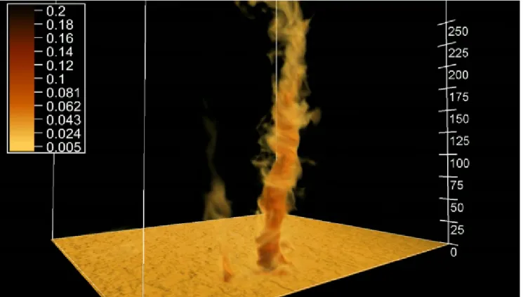
Refining the horizontal resolution in LES mostly impacts the size of simulated vortices (which become smaller), and the number of detected vortices (with more detections at higher resolutions; Raasch and Franke, 2011). However, Ito et al. (2013) showed that the results of Ito et al. (2010b) on the influence of background wind on dust devil formation, and the intensity of simulated dust devils, are basically left unchanged by refining the horizontal resolution from 50 m to 5 m. Weißm¨uller et al. (2016), using the model of Raasch and Franke (2011), showed that LES with mesh spacing of 1 m (cf. Figure 6) yielded dust devils with central pressure drops comparable to observed values. This result could not be obtained in the 2 m LES of Kanak (2005), and appears different from the results obtained by Ito et al. (2013). It is still unclear, nevertheless, if refining horizontal resolution alone is the only factor needed for obtaining realistic dust-devil-like vortices through LES. The simulations of Weißm¨uller et al. (2016) include a higher-order advection scheme and background winds, which might explain the differences with results reported in Kanak (2005). Furthermore, it still a matter of active research to determine the resolution at which the LES spectrum starts to significantly deviate from the theory, and what is the impact of the choice of the advection scheme on this resolution.
E(k)%
k%
π%/%Δ%
dust%%
devils%
Figure 5: The required horizontal resolution for dust devils in LES. Idealized spectrum of kinetic energy (E) as a function of wavenumber (k) as measured in the boundary layer (black line) or derived from LES (blue line). The red line denotes the wavenumber corresponding to the LES grid spacing ∆; the shaded area marks the typical size range of dust devils. Figure provided by co-authors Hoffmann and Raasch.
3.5
Considerations on vortex structure
The flow structure of well-developed dust devils was investigated in Kanak (2005) through theo-retical models of vortices, i.e., the Rankine and the Burgers-Rott models which consist in linking tangential velocity in the vortex to the radial distance from the vortex center (see Kurgansky et al. (2016) in this issue for further details). It was found that the Burgers-Rott model matches the convective vortices arising spontaneously in LES better than the Rankine model, because the internal flow structure within the vortex core cannot be approximated as a simple solid body rotation within the core (which is assumed in the Rankine model). Nevertheless, the findings of Kanak (2005) seem to indicate that the Rankine vortex is a good approximation for the simulated vortices at least within the radius of maximum wind. Thus, Ohno and Takemi (2010a) employed the Rankine vortex model to identify the near-surface flow structure within the vortex core. Most of the radii of maximum wind are within 1 – 2 horizontal grid points (with a mesh spacing of 3 m), with major ones being greater than 3 grid points. These large vortices have more substantial pres-sure deficits and enhanced vorticities on the order of 1 s−1. While the Burgers-Rott model appears more appropriate than the Rankine model to represent the flow structure within the vortex, Ohno and Takemi (2010a) shows that the latter is sufficient to conduct a statistical analysis from a large number of vortex samples.
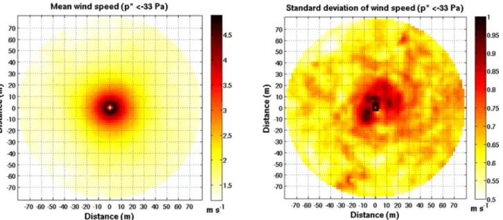
The question of the applicability of the Rankine model was also addressed recently using the high-resolution LES by Weißm¨uller et al. (2016) (see section 3.7). Figure 7 suggests that the tangential winds of vortices beyond the vortex wall are rarely as tangential, and the fall-off as steep or as uniform, as the Rankine model would suggest. Similar limitations of the Rankine model can
Figure 6: High-resolution terrestrial LES for dust devils. Animation of dust devils in the convective boundary layer using a virtual dust source. LES of dust devils performed by Weißm¨uller et al. (2016) using the model of Raasch and Franke (2011). This figure is extracted from a movie which can be found by following the link http://dx.doi.org/10.5446/9352
Figure 7: The structure of a convective vortex obtained with high-resolution terrestrial LES. Compos-ite of mean and standard deviation of 5 m wind speeds for 111 of the strongest vortices (central pressure < −33 hPa) using the high-resolution LES with no background wind in Weißm¨uller et al. (2016). Figure produced by co-author Jemmett-Smith (personal communication).
also be diagnosed from in-situ observations (Lorenz, 2014). Those are due to the interactions of the vortices with the convective ambient atmosphere, since convective vortices are mostly observed at the branches of the convective cell patterns (Kanak, 2005; Gheynani and Taylor, 2010), which generate local winds. Subsequently, only when vortices are mature (or on the rare occasions when they form in a locally weak wind region before moving away from those areas) are they likely to closely follow a Rankine model.
Interestingly, if the vortex intensity is increased, the vortex structure will change its form from a circular, single-celled flow to another regime (e.g. Rotunno, 2013). In the LES of Ohno and Takemi (2010a) and Ito et al. (2010b), it was demonstrated that an intense vortex has a celled structure which includes a downdraft at the vortex center – this type of double-celled structure was identified in observed dust devils (Bluestein et al., 2004, see also Murphy et al. (2016) and Fenton et al. (2016) in this issue). Thus, a transition from a single-celled to a double-celled structure is found for intense dust devils in both observations and LES – quite similar to what occurs in tornadoes, which are much stronger atmospheric vortices than dust devils (Rotunno, 2013). This suggests a similarity between high-intensity dust devils and low-intensity tornadoes from a viewpoint of vortex properties. This analogy could help to explain the “spiral-arm” structure of some convective vortices resolved by LES, see e.g. Figure 4, although this item is seldom discussed in the literature (Kanak, 2005). However, the analogy does not extend to intense tornadoes which undergo an additional transition from double-celled to multiple vortices, which most likely does not occur in the weaker CBL vortices that become dust devils.
3.6
Dust particles and convective vortices
Recently, the gap between simulating convective vortices versus predicting actual dust devils started to be overcome by LES coupled to dust emission schemes (Klose and Shao, 2012, see Section 2.5). Using this new modeling perspective, Klose and Shao (2013) adopted a systematic approach with a set of 15 LES with various background wind (initialized with logarithmic wind profiles for u∗ = 0.15, 0.3, and 0.5 m s−1) and atmospheric stratification settings (as specified by
constant surface sensible heat fluxes, Hs=-50, 0, 200, 400, and 600 W m−2, with the highest value
chosen to mimic strongly heated desert surfaces). The model runs were not set up with a particular focus on dust devils, but with the broader goal to investigate convective turbulent dust emission, of which convective vortices are a component. Klose and Shao (2013) found that the largest CBL dust emissions occur in micro-convergence lines, micro-downdrafts, and in the area of convective vortices (Figure 8). In a follow-up work, Klose and Shao (2016) repeated the model runs with a further developed and calibrated dust emission scheme (Klose et al., 2014), this time with a focus on dust entrainment by dust devils detected through a tracking algorithm based on a range of criteria for pressure drops (∆p = 0.05 − 0.25 hPa) and vorticity (0.1 − 1.0 s−1). Statistical analysis of dust emission in dust devils shows that dust devils occurring in a similar setting (i.e. same model run) can exhibit a wide range of dust fluxes. The maximum values reached in dust devils are determined by atmospheric stability. Dust devils occur most frequently at highly negative Richardson numbers (e.g. unstable stratification and weak mean winds) and exhibit a relatively longer duration than under other conditions. Although of shorter duration and less frequent, dust devils at weakly negative Richardson numbers (i.e. unstable stratification and relatively strong mean winds) can have larger dust emissions, as the stronger mean wind shear contributes to the lifting (see Rafkin et al. (2016) in this issue).
The simulations show that turbulent dust emission in dust devils is typically of the order of magnitude 102µg m−2s−1 (Figure 9), but can reach the order of magnitude 103µg m−2s−1, similar to that typically generated by saltation bombardment (Klose and Shao, 2016) and at the lower edge of that measured in dust devils in the field (Metzger et al., 2011, and see Chapter Murphy et al. (2016) in this issue). The additional inclusion of intermittent saltation (e.g., Dupont et al., 2013) in the turbulent dust emission scheme would lead to even larger fluxes, closer to those measured in the field (see Klose et al. (2016) in this issue for further discussion on fluxes associated with dust devils). The recent study of Klose and Shao (2016) shows that modeling dust devils through LES is possible, provided an appropriate dust emission scheme is included.
To complement those LES studies of dust emission, steady-state vortex models can be employed to address the transport of dust particles within the convective vortex. For instance, Gu et al. (2006) studied the trajectories of sand particles (diameter 100 to 300 µm) injected within a mature-stage swirling flow bearing similarities with dust devils. The resulting spatial distributions for the different grain sizes are summarized in Figure 10. The small particles move along with the main streamline of the updraft, while the large ones deflect outward from, and deposit beyond, the main core of the dust devil. In addition to the drag in the updraft, the centrifugal force exerted on the solid particles in the swirling air flow of dust devils is another key force component on the horizontal plane, which might explain the deflection of larger particles. Some of the ejected larger particles may be re-entrained into the rapid near-surface inflow, and be returned to the vortex. In effect,
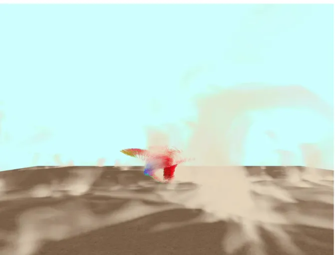
Figure 8: Turbulent dust emission simulated in a terrestrial LES, including the effect of a dust devil. Modeled dust concentration is visualized with a volume rendering approach. A particle-tracing is applied to illustrate a dust devil occurring in the simulation. Colors indicate the direction of particle movement. Modeling results are described in Klose and Shao (2013). This figure is extracted from a movie which can be found by following the link http://dx.doi.org/10.5880/SFB806.5.
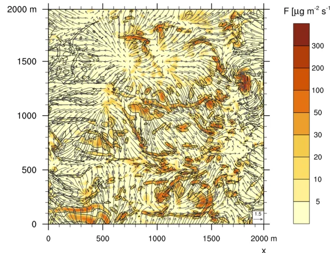
Figure 9: Flux of dust particles associated with turbulent structures resolved in terrestrial LES. Turbulent wind speed (vectors, in m s−1) and instantaneous turbulent momentum flux (black contour lines at 1 N m−2) at 10 m height together with turbulent dust emission F (shaded, in µg m−2s−1). The strongest turbulent dust emissions occur at micro-convergence lines (e.g. at coordinates x = 850 m, y=800 m), micro-bursts (e.g. at coordinates x = 800 m, y=1700 m), and vortices (e.g. at coordinates x = 1800 m, y=1400 m). Figure published in Shao et al. (2015), used with permission.
Figure 10: Dust lifting patterns in a dust devil. 1-track of fine dust grains; 2-track of medium grains; 3-track of large grains; 4-small vortices induced by the interaction of different sized grains; 5-general pattern of interactions. Figure published in Gu et al. (2006), used with permission.
such particles may move circularly on the flanks of the dust devil until the updraft decays and the drag is not enough to lift them. Large particles thus draw the “outer boundary” of the dust devil, while smaller-size particles spiral up within the dust devil core and draw an “inner boundary”. Medium-sized particles adopt an intermediate behavior. This implies that size discrimination is at play within dust devils (as was hypothesized by Ferrel in 1881, see Lorenz et al. (2016) in this issue), and that mostly smaller particles are being helically raised within (or even above) the CBL. LES has not yet reached the level where high-resolution dynamical integration can be coupled to reliable dust emission scheme, in order to produce a very detailed simulation of the inner workings of dust devils. However, this goal is within reach in the near future given the recent body of work on this topic (e.g. Klose and Shao, 2016). This will confirm the conclusions drawn from the aforementioned idealized vortex modeling with particle injection (Gu et al., 2006), which does not account for a complete distribution of particle sizes, and lacks smaller-scale turbulent components that can be resolved in high-resolution LES. Nevertheless, LES would still not be appropriate to resolve the individual dynamics of transported particles (and collisions between them), for which idealized modeling with a pre-existing vortex will still be of great value.
3.7
A dust-devil parameterization based on LES?
The preceding discussions make clear that LES studies for the terrestrial CBL recently progressed from reproducing spontaneous convective vortices towards obtaining predictions for real dust devils,
i.e. convective vortices that have gained the capability to lift and transport dust particles (e.g. Klose and Shao, 2013). Since obtaining in-situ field observations for a population of dust devils remains a difficult task (Lorenz, 2014, and see Murphy et al. (2016) and Lorenz and Jackson (2016) in this issue), the relative success of LES in representing dust devil-like vortices in recent years highlights a unique point in dust devil research, where LES can be used as a tool to improve our understanding and representation of these phenomena.
It is now possible to envision the use of LES to design a physical model (“parameterization”) to account for the effects of dust devils, notably on the dust cycle, in GCM and RCM which cannot resolve those phenomena – and are unlikely to do so within the foreseeable future. This approach is distinct from the earlier dust devil parameterizations based on thermodynamical arguments (Renno et al., 1998, see also Klose et al. (2016) in this issue). Using relatively large domains (on the order of 4 km in the horizontal) and high resolutions (down to 2 m in the horizontal), a population of dust devil-like vortices, with different sizes and strengths, can be investigated under different initial conditions (Weißm¨uller et al., 2016). Moreover, Klose and Shao (2016) showed that relating to the Richardson number the dust-devil emission and counts predicted through LES is a valuable means to estimate regional and global dust transport by dust devils. A fully mature dust devil parameterization based on LES has yet to emerge, however. One has to represent a full range of dust devil behaviour changes caused by different meteorological (i.e., ambient wind, temperature profile) and surface conditions (i.e, soil properties, terrain and roughness). This requires numerous, computationally expensive simulations to fully explore these effects. To further complicate matters, an interplay of mechanisms contribute to dust emission by dust devils: saltation bombardment, ∆P effect (see Neakrase et al. (2016) in this issue), direct emission by CBL gusts (see Section 3.6), and electrification of sand and dust particles (e.g., Huang et al., 2008, and see Harrison et al. (2016) in this issue for further details). Each of these phenomena warrants further investigation – some of them possibly with LES – before a dust devil parameterization could be used in GCM and RCM, leading to improved estimates of their contribution to the global mineral dust budget, which is a key component of the Earth system (Knippertz and Stuut, 2014).
4
LES for Mars
4.1
First LES studies and properties of simulated vortices
As is summarized in the introduction, studying convective vortices and dust devils on Mars through LES was part of a broader body of work aiming to understand CBL dynamics on Mars: daytime CBL growth, polygonal cells, thermal up/downdrafts and convective vortices (Rafkin et al., 2001; Toigo et al., 2003; Michaels and Rafkin, 2004; Sorbjan, 2007; Richardson et al., 2007; Tyler et al., 2008; Spiga and Forget, 2009; Spiga et al., 2010; Gheynani and Taylor, 2011). Here we only review LES studies where the properties of modeled convective vortices are discussed (Table 2). Those modeling studies of the CBL started when quantitative in-situ and orbital measurements complemented the early detection of dust devils structures in imagery (Thomas and Gierasch, 1985; Schofield et al., 1997; Malin and Edgett, 2001, see Murphy et al. (2016) and Fenton et al. (2016) in this issue for detailed discussions, and Figure 1 upper right for an example image of a
dust devil).
The pioneering two-dimensional Martian LES by Odaka et al. (1998) provided insight into CBL growth and associated vertical velocities, but was not suitable to study the emergence of convective vortices (because, e.g., vortex stretching is not being permitted in two-dimensional dynamical integrations). The first successful attempt by Rafkin et al. (2001) to perform three-dimensional LES on Mars reports the emergence of convective vortices (Figure 11) at the boundaries of open polygonal cells formed by narrow updrafts (and broad downdrafts in the middle of each cell, dictated by the conservation of mass). The behavior of convective vortices with time was discussed in more detail in Michaels and Rafkin (2004). Convective vortices are predicted from morning (local time 08 : 30) to late afternoon when the CBL collapses (local time 17 : 00). In the early afternoon, when the convection is at its most vigorous, LES show numerous convective vortices of diameter 100 − 1000 m in the first hundred meters above the surface. However, only a small fraction of these vortices resolved through LES evolved into structures in cyclostrophic equilibrium comparable to the observed dust devils, which have a vertical extent of 60% of the CBL and exhibit no preferred direction of rotation.
Using the LES model of Michaels and Rafkin (2004), and accounting for dust lifting and aerosol transport (see section 2.5), Michaels (2006) was able to show that convective vortices would indeed be conducive to the formation of dust devils, if dust material is available at the surface. This would indeed account for the observed tracks along the ground of darker material, where bright dust is removed by vortices (see Figure 12, and Reiss et al. (2016) in this issue). Michaels (2006) relates the cycloidal path followed by the simulated dust devil in Figure 12 to the dynamically-evolving convective motions being similar in magnitude to the weak background wind set in his simulation; LES with stronger background wind predict a more uniform rate of translational motion for the simulated convective vortices.
Toigo et al. (2003) dedicated their paper to an in-depth analysis of convective vortices in Mar-tian LES (Figure 13), by means of a model using a distinct dynamical core than Rafkin et al. (2001) and Michaels and Rafkin (2004). They noticed a great similarity with the equivalent terres-trial phenomena (Kanak et al., 2000; Kanak, 2005), including the formation of vortices preferably at the intersection of the convective cells. A plausible scenario to account for this is the tilting into the vertical of the horizontal vorticity resulting from temperature contrasts in the lowermost levels of the CBL (the same diagnostic is proposed in Michaels and Rafkin, 2004). The detailed LES analysis enabled Toigo et al. (2003) to distinguish the contribution of each term in the TKE equation. Convective vortices result from an equilibrium between production of TKE by buoyancy and removal of TKE via both advection and dissipation towards the smaller eddies. Toigo et al. (2003) found a high sensitivity of the activity of the dust devil-like vortices to the background wind. Once formed, a convective vortex in LES obeys a structure that can be described to first order by the thermodynamic theory of Renno et al. (1998) (see Rafkin et al. (2016) and Kurgansky et al. (2016) in this issue).
The properties of modeled convective vortices in the aforementioned LES studies are summa-rized in Table 2. Despite the range of simulated values obtained in the various studies, they agree at the order of magnitude level: simulated convective vortices exhibit updraft velocities up to about 10 m s−1, tangential velocities from 10 to 20 m s−1 (compliant with the orbital measure-ments of Choi and Dundas, 2011), and central pressure drops of about a couple Pascal (consistent
Figure 11: Convective vortices in Martian LES. Dust-devil-like circulations captured during the Large-Eddy Simulation of Rafkin et al. (2001). Fields are shown on a portion of the horizontal domain at about 10 m above the surface: vertical vorticity and vector winds (top), wind speed and vector winds (bottom). The prescribed background wind velocity has been substracted to obtain the displayed wind vectors. Figure published in Rafkin et al. (2001), used with permission.
Figure 12: Dust devil track predicted by Martian LES. Simulated track made by a clockwise rotating dust devil (movement is from left to right; approximately 1100 local time; the x-axis and y-axis represent the indices of horizontal grid points). Depth of net surface dust reservoir change is shaded (mm; negative values denote dust removal). Red markers indicate the approximate position of the surface center of the vortex (shown every 75 seconds), and black contours indicate the approximate surface radial extent of the vortex core walls (updrafts; the small, unassociated contour near the figure center is a separate, smaller vertical convective vortex). Figure published in Michaels (2006), used with permission.
Figure 13: The vertical structure of one convective vortex obtained in Martian LES. High-resolution Large-Eddy Simulation (∆x = 10 m) of the “no wind” simulation dust devil of Toigo et al. (2003). Here is plotted a vertical slice through the center of the dust devil. Background color shows the tangential wind speed. Black contours show the pressure perturbation in Pa, reaching a maximum difference near the surface of about 1 Pa less than the background. Yellow contours show potential temperature in K, and the warm core of the dust devil. White contours show upward wind velocity in m s−1. Upward wind velocity peaks at the walls of the dust devil, and the decrease in upward velocity can be seen in the center of the dust devil core. Figure published in Toigo et al. (2003), used with permission.
Paper Dyn. dx Nx,y Z Nz w0 v0 P0 ζ core (m) (km) (m/s) (m/s) (Pa) (s−1) Rafkin01 RAMS 100 180 9 36 10 10 2 0.3 Toigo03 MM5 10 200 6 140 7 9 1 0.06 Toigo03b MM5 100 100 7.5 57 7 5 - -Michaels04 RAMS 30 200 2.3 61 5 10 2 0.2 Michaels06 RAMS 25 102 8 120 12 19 6.5 -Spiga09 WRF 100 150 9.5 71 8 10 1.5 -Spiga10b WRF 50 145 12 201 12 10 2 -Gheynani11 NCAR 25 200 10 60 4 15 2.5 0.7 Nishizawa16 SCALE 5 4000 21 4000 10 20 4.2 2
Table 2: Same table as Table 1 for published LES studies in Martian conditions. The LES by Rafkin01, Toigo03, Michaels04, Michaels06 were run for environmental conditions typical of Meridiani Planum; Toigo03b and Spiga09 of the plain within Gusev crater; Spiga10b of Amazonis Planitia; Gheynani11 of Vastitas Borealis; and LES by Nishizawa16 were run with idealized Martian radiative forcing.
with measurements on board the Martian landers, e.g. Schofield et al., 1997; Ellehoj et al., 2010, although the pressure drops > 5 − 10 Pa required to form dust devil tracks and to cause solar panel clearing events according to Lorenz and Reiss (2015) are not reproduced by existing LES). Comparing Table 2 with Table 1 appears to confirm that Martian dust devils are more intense than their terrestrial counterparts, when considering velocities and presure drop scaled to the mean surface pressure on each planet. Those estimates have been bolstered by other LES studies performed with distinct models and in distinct locations (Toigo and Richardson, 2003; Spiga and Forget, 2009; Spiga and Lewis, 2010; Gheynani and Taylor, 2011). Not all the studies report the duration of convective vortices in LES, but the most distinctive and extreme predicted vortices are estimated to last about a few thousands of seconds (Toigo and Richardson, 2003; Spiga and Forget, 2009).
An interesting complement to this whole body of work based on Category 3 LES (see section 2.4) is provided by the Category 1 LES for Mars reported by Kanak (2006) who investigated the minimum physical requirements for vortex formation in the Martian CBL. Despite the arguably very idealized setting compared to usual Mars LES (no radiative processes, simpler surface layer and sub-grid scale parameterizations, little to no background wind), Kanak (2006) showed that convective vortices still arise with similar properties as those predicted by more sophisticated LES – and that the mechanism by which they acquire rotation is, as discussed by others, deeply rooted in the CBL dynamics (i.e. dust devils do not develop independently from the CBL growth, but as a part of it). The fact that every Martian lander (see Murphy et al. (2016) in this issue) was able to detect pressure drops characteristic of convective vortices supports their ubiquitous presence in Mars LES. This confirms that studying convective vortices is a means to more generally study CBL processes, because those develop wherever the CBL grows deep enough.
4.2
Regional variability
Determining tendencies for the regional variability of dust devils from the LES studies reported in Table 2 is difficult. First and foremost, as is indicated in Table 2, LES settings in various studies are too different (horizontal resolution, background wind). But even keeping this caveat in mind, the actual regional variability in dust devils – e.g. what makes Amazonis Planitia such a propitious place for dust devil occurrence (Fisher et al., 2005), or the fact that the Spirit rover witnessed far more dust devils than the Opportunity rover (Greeley et al., 2006) – remains an open question that LES has not addressed yet. A plausible explanation for this is the regional variability of dust availability, which is not accounted for in existing Martian LES. Another possibility is that the occurrence of dust devils, as well as their height and spacing Fenton and Lorenz (2015), somehow relates to the intensity of convective vortices – which makes it possible for existing LES to solve this scientific issue. Although this problem remains unsolved thus far, recent studies were able to draw a few preliminary conclusions or perspectives.
Radio-occultation measurements showed that the Martian CBL appeared to extend to higher altitudes over high plateaus than in lower altitude plains, despite similar surface temperatures in the considered regions (Hinson et al., 2008). Spiga et al. (2010) showed that these dramatic regional variations of CBL depth are qualitatively and quantitatively predicted by LES by accounting for the regional differences in the surface properties and incoming sunlight. Those regional variations of CBL depth arise because the prominent radiative control of the Martian CBL (as opposed to sensible heat driving the terrestrial CBL) makes the intensity of convective motions correlated with the inverse surface pressure: the LES of Spiga et al. (2010) hence predict stronger near-surface horizontal winds and CBL vertical winds over high plateaus than over lower plains. This led to a plausible explanation as to how dust devils would be found at the Martian volcanoes’ summit where atmospheric density would be too low to allow for dust to be lifted from the surface (Reiss et al., 2009).
Most Mars LES models are still rather idealized (see section 2.2) and, without the forcing of the regional and large-scale circulation, should not be assumed too representative for any specific location on the planet – especially if the region is characterized by uneven topography or strong contrasts in surface thermophysical properties. For terrestrial LES, neglecting the larger-scale cir-culation is typically seen as a reasonable approach, although similar caveats apply if significant mesoscale circulations are present. For LES on Mars, although the CBL depth is primarily con-trolled by incoming sunlight and surface thermophysical properties, both the regional circulations (e.g. slope winds) and the strong atmospheric thermal tides can play very important roles in the diurnal growth of the CBL:
• Strong atmospheric thermal tides produce large diurnal and semidiurnal amplitudes in the surface pressure cycle. This leads to large and rapid variations in the atmospheric horizontal pressure gradient. When this rapidly varying forcing interacts with the growth of a deep Martian CBL, the result can vary greatly when compared to a case without such forcing. Using a prescribed time- and height-dependent geostrophic wind (a theoretical wind that would exist in an exact balance between the pressure gradient force and the Coriolis effect) computed from RCM for the Phoenix landing site, Tyler et al. (2008) showed that daytime convection was stronger than with a fixed uniform background wind, which leads to the
formation of a deeper CBL. Regional circulation can produce sizeable differences in LES results, but the effect thereof on dust devil activity remains to be quantified.
• Whether convergence/divergence exists in the local circulation is another important aspect. In crater circulations, daytime convergence at the height of the surrounding terrain above the floor of the crater produces a temperature inversion due to the adiabatic warming of widespread subsidence (Tyler and Barnes, 2013; Tyler and Barnes, 2015). This provides a plausible explanation for the small CBL depths assessed by imagery from the Curiosity rover operating within Gale Crater (Moores et al., 2015). Given the topography of Mars, and the strong slope flows that develop, this reality poses an additional problem to LES on Mars for specific locations. One investigative path forward may be to add a heating term in the LES that mimics the adiabatic warming of subsidence. As is the case for the preceding point, the impact of this on dust devil activity (and a possible explanation for the lack of observed dust devils by Curiosity, see Murphy et al. (2016) in this issue) is yet to be determined.
4.3
Sensitivity exploration
Recent work on LES for Mars has explored the sensitivity of earlier results to various modeling parameters. This was discussed notably by Fenton and Michaels (2010), although the aim of their set of LES experiments at two distinct seasons, and using different conditions of background wind, was to determine the velocity distribution of near-surface CBL winds, rather than to focus on con-vective vortices alone. However, the tail of the wind distribution provides direct information on the strength of near-surface winds imposed by convective vortices, and possibly dust devils since maximum wind speeds in the LES of Fenton and Michaels (2010) do exceed the stress threshold to mobilize sand grains on Mars. Fenton and Michaels’ LES show that maximum friction velocities increase with incoming sunlight and background wind, although simulations without background wind also produce a high speed wind tail that exceeds the local saltation stress threshold. Interest-ingly, the LES using strong uniform winds with superimposed wind shear yield a wind distribution which departs significantly from the Weibull distribution (unlike the LES with lesser background winds). Since convective vortices are associated with the tail of the wind distribution, those results could indicate, similarly to terrestrial studies (Section 3.3), that a significant rise in large-scale and regional winds could impact the occurrence of dust devils.
A notable sensitivity study on convective vortices predicted by Martian LES was carried out recently by Gheynani and Taylor (2011), who used a higher resolution of 25 m (see Table 2). Gheynani and Taylor (2011) performed LES with various background wind speeds (0,4,8 m s−1) and two distinct assumptions on radiative forcing (comparing Category 1 LES vs. Category 2 LES, as defined in Section 2.4). Their study shows a decrease of vortex populations in windy conditions, finding that mean vortex tangential velocity increases accordingly with both pressure drop and vorticity. Gheynani and Taylor (2011) add to the current knowledge the result that smaller and more intense vortices form in LES with larger background wind. This indicates that background wind destroys weak vortices – or limits their formation, and only vortices with enough momentum will survive in windy conditions (see Rafkin et al. (2016) in this issue for detailed discussions on the relationship of background wind to dust devil size and number). The LES
Figure 14: Properties of simulated convective vortices in Martian LES with distinct model assump-tions. Vortices’ maximum (square) and minimum (diamond) property values, and the average (circle) of (a) vorticity (b) diameter (c) pressure drop (d) temperature increment (e) tangential velocity (f) vertical velocity, dur-ing the last 45 min (1100–3800 s) of simulation time at 20 m above the surface. Blue stands for clockwise vortices, red stands for counter-clockwise vortices. Figure published in Gheynani and Taylor (2011), used with permission.
of Gheynani and Taylor (2011) with and without radiative forcing (Category 1 vs. Category 2 LES) indicate that vortices’ vertical velocities slightly increase when radiative forcing is taken into account. The differences between both cases in vorticity, pressure drops, and tangential velocities is only about 1 − 5 % (Figure 14). Thus, the effect of including radiative forcing in Gheynani and Taylor (2011) was relatively insignificant, if not negligible (confirming the results in Kanak, 2006, cf. section 4.1). This implies that, while radiative forcing is key on Mars to obtain appropriate CBL structure and dynamics (see e.g. Spiga et al., 2010), it is less of a requirement to obtain correct dust devil properties and statistics on Mars. This also suggests a closer similarity than expected with terrestrial LES (see also Gheynani and Taylor, 2010). However, further investigation is warranted since the LES of Gheynani and Taylor (2011) were only hour-long runs which did not account for CBL growth during the day, and no radiatively active dust was being advected into the simulated vortices.
4.4
Perspectives and challenges
The ability of Martian LES to reproduce convective vortices that bear resemblance to actual dust devils opens interesting perspectives. One of them is the possibility to simulate electrostatic dis-turbances and the electric field induced by dust devils through triboelectric charging of saltating and colliding sand and dust particles (e.g. Renno et al., 2003, see also Harrison et al. (2016) in this issue). Following Michaels (2006), Barth et al. (2014) coupled a detailed aerosol model (operating on discrete mass bins) to the LES model of Rafkin et al. (2001) run at an improved horizontal resolution of 33 m, and incorporated dynamic spatial redistribution of initially charged dust par-ticles in order to evaluate the possibilities for electric fields generated within the dust devils in their LES. Using the Microscopic Triboelectric Simulation (MTS; see Harrison et al. (2016) in this issue for further description), they added tracers to represent the moments of a distribution of particle charges across each mass bin. As the dust was lifted and redistributed spatially by both convective vortices and gravitational settling, the charge density at each grid point would also evolve. They found consistency with observations of terrestrial dust devils in that the smaller, negatively charged particles tended to almost exclusively occupy the top portions of the vortex, while the larger, positively charged particles were more likely to fall to the surface. This charge separation allowed for the calculation of electric fields using Poisson’s equation. In addition to electric fields generated by the dust devils, Barth et al. (2014) also noted that gust fronts along the boundaries of the convective cells could lift substantial amounts of dust and thus result in larger-scale electric fields. Given an initial grid box size of 100 m2 in the horizontal, these gust front E-fields tended to overwhelm anything produced within the dust devil. The above mode of grain moving, mixing and collision could develop a small-size (lighter) grain domain aloft and a near-surface large-size (heavier) grain domain (i.e. grain mass stratification), and thus produce strong electric fields within dust devils. The dust cloud has a macroscopic electric dipole moment oriented in the nadir (downward) direction, which might play a significant role in dust sourcing.
In a more general scope, perspectives and challenges for Martian LES somewhat mirror those for terrestrial LES (Section 3.7), although observational limitations in the Martian case prevent dust emission schemes as sophisticated as the Earth’s (Klose et al., 2014, see Section 3.6) to be calibrated. As is the case on the Earth, progress is being made that may soon lead to