HAL Id: hal-01622160
https://hal.archives-ouvertes.fr/hal-01622160
Submitted on 25 Oct 2017
HAL is a multi-disciplinary open access
archive for the deposit and dissemination of
sci-entific research documents, whether they are
pub-lished or not. The documents may come from
teaching and research institutions in France or
abroad, or from public or private research centers.
L’archive ouverte pluridisciplinaire HAL, est
destinée au dépôt et à la diffusion de documents
scientifiques de niveau recherche, publiés ou non,
émanant des établissements d’enseignement et de
recherche français ou étrangers, des laboratoires
publics ou privés.
Tools for Robustness in Dynamic Dial-a-Ride Problem
Samuel Deleplanque, Alain Quilliot
To cite this version:
Samuel Deleplanque, Alain Quilliot. Tools for Robustness in Dynamic Dial-a-Ride Problem. Studies in
Computational Intelligence, Springer Verlag, 2015, Recent Advances in Computational Optimization.,
580, pp.35-51. �10.1007/978-3-319-12631-9_3�. �hal-01622160�
Tools for Robustness in Dynamic Dial-a-Ride
Problem
Samuel Deleplanque1and Alain Quilliot1
LIMOS CNRS Laboratory, LABEX IMOBS3, Clermont-Ferrand 63000, France
Abstract. The Dial-a-Ride Problem (DARP) models an operation re-search problem related to the on demand transport. This paper intduces one of the fundamental features of this type of transport: the ro-bustness. This paper solves the Dial-a-Ride Problem by integrating a measure of insertion capacity called Insertability. The technique used is a greedy insertion algorithm based on time constraint propagation (time windows, maximum ride time and maximum route time). In the present work, we integrate a new way to measure the impact of each insertion on the other not inserted demands. We propose its calculation, study its behavior, discuss the transition to dynamic context and present a way to make the system more robust.
1
Introduction
Today, the Dial-a-Ride Problems are used in transportation services for elderly or disabled people. Also, the recent evolution in the transport field such as connected cars, autonomous transportation, and the emergence of the shared service might need to use this type of problem at much larger scales. But this type of transport is expensive and the management of the vehicles requires as much efficiency as possible, however the number of requests included in the vehicles planning can vary depending on the resolution used.
In [15], we solve the DARP by using constraint propagation in a greedy insertion heuristic. This technique obtains good results, especially in a reactive context, and is easily adaptable to a dynamic context. But, each demand is inserted one after another and the process does not take into account the impact of each insertion on the other not inserted demands, and so, in a dynamic context, the future demands. In this work, we present a measure of an insertion capacity named Insertability.
We introduce its calculation by integrating indirectly the impact of an inser-tion on the time constraints (time windows, maximum route time and maximum ride time) of the other demands.
This measure may be used in different steps of the resolution: selection of the demand to insert, selection of the insertion parameters, taking the decision to exclude a demand, and in the process making the service time. These four uses may be related to static as well as dynamic contexts. The main goal is to insert the current demand in a way to create routes which will be able to insert the future demands.
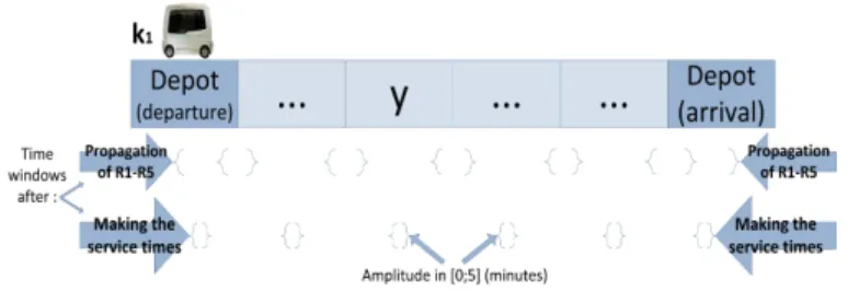
This paper is organized in the following manner: after a literature review, the next section will propose a model of the classic DARP. Then, we will review how to handle the temporal constraints with a heuristic solution based on insertion techniques using propagation constraints. We will continue by explaining the way to measure the Insertability, a calculation based on the evolution of the time windows after an insertion. Then, we will give some other uses of this measure including the setting of the service times which minimize the time windows (cf. Figure 1). In the last part of the paper, the computational results will show the efficiency of our Insertability’s measure and we will report the evolution of the number of demands inserted in a resolution of some instances’ sets.
Fig. 1. Times windows contraction
2
Literature review
The first works of the transportation optimization problem are related to the Traveling Salesman Problem ([9]). Since that time, other transportation prob-lems have emerged as the vehicle routing and scheduling probprob-lems, and also the Pick-up and Delivery Problem (PDP). Based on the PDP, the DARP which has been studied since the 1970’s. The Dial-a-Ride problem is related to the on de-mand transportation which is more often manage in a dynamic context, unlike the PDP.
There are a number of integer linear programmings [6], but the problem complexity is too high for using it in a real context. Indeed, it is an NP-Hard because it also generalizes the Traveling Salesman Problem with Time Windows (TSPTW). The optimal solution can be find only for small instances [8]. There-fore, and more specially for the dynamic context, the problem must be handled through heuristic techniques.
For the static DARP, [4] is an important study on the subject. In this work, they use the Tabu search metaheuristic to solve the problem. Starting from an initial solution, the resolution process moves from a solution to another in a neighborhood. The operator which executes these moves will take a demand already assigned to vehicle k and insert it in another vehicle k0. The Tabu list saves each application of the operator in order to avoid cycling. The insertion
parameters of the demand (for the origin and the destination) are chosen in order to minimize the total distance. They don’t take in account all the constraints of the DARP during the process. They reach a feasible solution by integrating penalties in the performance criteria.
Other techniques are efficient for the static DARP. Dynamic programming (e.g. [10] and [3]) or variable neighborhood searches (VNS) (e.g. [11] and [12]) gived good solutions.
A basic feature of DARP is that it usually derives from a dynamic context. Therefore, algorithms for static DARP should be designed in order to take into account the fact that they will have to be adapted to dynamic and reactive contexts, which means synchronization mechanisms, interactions between the users and the vehicles, and uncertainty about for-coming demands ([7]).
[13], and [14] later, developed the most used technique in dynamic context or in a real exploitation is heuristics based on insertion techniques. These techniques give good solutions even if the people’s requests have to be taken into account in a very short period of time.
[1] adapt the Tabu search of [4] to the dynamic DARP and a parallel en-vironment. Indeed, each replication is independent in order to be executed on different CPU cores ([1]). In fact, the operator moving from a solution to another uses simple insertion technique. Other recent works are made on the dynamic Dial-a-Ride problem, and in particular about the problems of reactivity. For in-stance, in [2], they develop an algorithm able to take in account requests in real time. The requests are given directly to the driver, thus the decision is made immediately. Therefore, they describe the resolution process launched each time a new request appears in the system.
3
Mathematical model
We first introduce the standard mathematical model for a single criterion DARP. The objective here is the minimization of the total distance. The DARP is defined by a transit network G = (V, E), which contains at least two nodes Depot (depar-ture and arrival), and whose arcs e ∈ E are endowed with riding times equal to the Euclidean distance between two nodes of V , i and j, DIST (i, j) ≥ 0. A fleet VH of K vehicles k with a capacity CAP and a Demand set D = (Di, i ∈ I). Any demand (or request) Diis defined as a 6-uple Di= (oi, di, Di, F (oi), F (di), Qi), where:
– oi∈ V is the origin node of the demand Di and the set of all the oi is DE . di∈ V is the destination node of the demand Di and all the di are gathered in AR;
– F (oi) and F (di) are respectively the time windows for oi and oi of the demand Di. F .MIN and F .MAX are the two bounds of a window;
– ∆i≥ 0 is an upper bound on the ride time of the demand i; – Qi is the Di’s load such that qoi = Qi= −qdi.
We denote by tk
x the time at which the vehicle k begins service in x, x ∈ V . Also, δj, j ∈ V , is the non-negative service time necessary at the node j and ∆k is the maximum route time for the vehicle k.
Then, we consider in G = (V, E) all the nodes corresponding to the oi ∈ V and di∈ V such that V = DE ∪ AR ∪ {0, 2 |D| + 1} with {0, 2 |D| + 1} the two depot nodes respectively for the departure and the arrival, oi ∈ {1.. |D|}, and di∈ {(|D| + 1)..(2 |D|)}. Moreover we denote by V0the set V without the depot nodes (i.e. V0= DE ∪ AR) and by ζk
j the total load of the vehicle k leaving the node j, j ∈ V .
Dealing with such an instance means planning the handling demands of D, by the fleet VH , while taking into account the constraints which derive from the technical characteristics of the network G, of the vehicle fleet VH , and of the 6-uples Di= (oi, di, Di, F (oi), F (di), Qi), and while optimizing some performance criterion which is usually minimizing the total distance or a mix of an economical cost (point of view of the fleet manager) and of QoS criteria (point of view of the users).
Let xk
ij a boolean equals to 1 if the vehicle k travels from the node i to the node j. Then, based on [5], the mathematical formulation is the following mixed-integer program : MinX k∈K X i∈V X j∈V DIST (i, j)xkij (1) subject to X k∈K X j∈V0 xkij = 1, ∀i ∈ V0 (2) X j∈V0 xkij − X j∈V0 xk|D|+i,j = 0, ∀i ∈ DE , k ∈ K (3) X j∈DE xk0j= 1, ∀k ∈ K (4) X j∈V0 xkji− X j∈V0 xkij = 0, ∀i ∈ V0, k ∈ K (5) X i∈AR xki,2|D|+1= 1, ∀k ∈ K (6) tkj ≥ (tk
i + δi+ DIST (i, j))xkij, ∀i ∈ V, j ∈ V, k ∈ K (7) ζjk ≥ (ζk
i + qj)xij, ∀i ∈ V, j ∈ V, k ∈ K (8) DIST (i, |(D)| + i) ≤ tk|(D)|+i− (tki + δi) ≤ ∆i, i ∈ DE (9) F .MINi≤ tki ≤ F .MAXi, ∀i ∈ V, k ∈ K (10)
tk2|D|+1− tk 0 ≤ ∆
ζik ≤ CAPk (12) xkij ∈ {0; 1}, t ∈ R+ (13) The program above is a three index formulation (report to [5] for more expla-nations about the objective function (1) and the constraints (2)-(13)), it exists in literature several other mathematical formulations for the DARP, even some with two index formulation [6]. But, the complexity of all these linear programs doesn’t allow finding an exact solution with a solver, the operation is too time consuming.
All along this work, we are going to deal with homogeneous fleets and with nominal demands, and we shall limit ourselves to static points of view but our insertion process allows flexibility for using it in a dynamic context. Still, we shall pay special attention to cases when temporal constraints are tight.
4
A greedy insertion algorithm
This section explains the techniques used to solve a static DARP instance. In our framework, the routes are saved in lists Γk surrounding by two depot nodes (one for the departure on the other for the arrival) with k a vehicle of the fleet V H (cf. Figure 1). For any sequence (or list) Γk we set:
– for any z in Γk, Succ(Γk, z) = Successor of z in Γk and Pred(Γk, z) = Predecessor of z in Γk ;
– for any z, z0 in Γk, z k z0 if z is located before z0 in Γk and z =k z0 if z k z0 or z = z0.
We also defined the T win function such that, for any node oi (respectively di) which appears in Γk, the node T win(oi) = di(and T win(di) = oi). The twin of a depot node is the other depot node in the same list.
In [15], we present an insertion greedy algorithm based on constraint prop-agation in order to contract time windows according to the time constraints of the DARP.
An insertion which does not imply constraint violation is said valid if Γ = ∪k∈KΓk, the resultant collection of routes, if load-valid and time-valid. A route is load-valid if the capacity is not exceed, so, the load-validity is obtained if ChTk(x) ≤ CAP with ChTk(x) =Py =
kxqy, x and y nodes in the route k. The
time-validity is obtained if there is no violation of the time constraints modeling by, for each demand i, i ∈ D, ∆i the maximum ride time, ∆k, k ∈ K the maximum route time and the constraints modeled by each time window F (oi) = [F .min(oi), F .max (oi)] and F (di) = [F .min(di), F .max (di)]. The service time δj of each node j ∈ V and origin of an arc e ∈ E is added in the DIST matrix, but without considering the departure depot nodes. Checking the load-validity on Γ = ∪k∈KΓkis easy, and we show the efficiency of the constraint propagation in order to prove to time-validity after each planned insertion once the load-validity is proved. According to a current time window set FP = {FP (x) = [ FP .min(x),
FP .max(x)], x ∈ Γk, k = 1..K} the time-validity may be performed through propagation of the five following inference rules Ri, i = 1..5 in a given route Γk: for each (x,y) pair of nodes such that y = Succ(Γk, x):
– R1 :
FP .min(x) + DIST (x, y) > FP .min(y) |=
(FP .min(y) ← FP .min(x) + DIST (x, y)); (FNodeModif ← y)
– R2 :
FP .max (y) − DIST (x, y) < FP .max (x) |=
(FP .max (x) ← FP .max (y) − DIST (x, y)); (FNodeModif ← x)
if (y = Twin(x)) and (x Γ y):
– R3 :
FP .min(x) < FP .min(y) − ∆i |=
(FP .min(x) ← FP .min(y) − ∆i); (FNodeModif ← x)
– R4 :
FP .max (y) > FP .max (x) + ∆i |=
(FP .max (y) ← FP .max (x) + ∆i); (FNodeModif ← y)
and for each x, x ∈ Γk, k = 1..K:
– R5 : FP .min(x) > FP .max (x) |= REJ ET ← true.
These 5 rules are propagated in a loop while there no time windows exists FP modified at the last iteration, i.e. once F N odeM odif is empty. In the R3 and R4 rules, the ’∆i’ is replaced by ’∆k’ if the pair of nodes (x,y) are depots. The tour Γk, k = 1..K, is time-valid according to the input time window set FP if and only if the REJET Boolean value is equal to false as initialized at the beginning of the process. In such a case, any valid -time value set t related to Γk and FP is such that: for any x in Γk, t(x) is the service time in FP (x).
The greedy insertion algorithm includes this propagation constraint tech-nique in order to evaluate each possible insertion. Each iteration of the algorithm selects one demand according to the number of vehicle able to integrate it. Once a demand is selected, the process chooses the best insertion’s parameters that are the vehicle and the location of the origin and destination nodes. These pa-rameters are chosen according to the smaller evolution of the routes costs (like the total distance in the mathematical model). The selection of the demand and
the parameters are made in a non-deterministic way (among a small set of the best variables). Then, we are allowed to include our process in a Monte Carlo scheme. The Figure 2 summarizes the general algorithm with P the number of replications resolving a DARP instance.
Fig. 2. The Monte-Carlo Process
5
Insertability optimization
In the above algorithm, each iteration selects a demand, and then, it finds the way to insert while minimizing the total cost. This greedy algorithm does not take in account the impact of this actual insertion on the future demands inte-gration, but only the effect on the demands already inserted. In this section, we introduce a Insertability calculation by integrating this impact of an insertion re-lated to the time constraints (time windows, maximum ride time and maximum route time).
During the insertion process, the state of the system is given by:
– a set of demands D − D1 already integrated in the routes, and D1 is the set of demands not inserted,
– a collection Γ = ∪k∈KΓk of routes including a list of nodes related to the Depot, origin and destination nodes,
– a exhaustive list of insertion’s parameters sets. Each set gathers 5 elements : k the vehicle, i the demand, (x, y) the pair of insertion nodes (locating respectively oi between x and the successor of x, and di between y and the successor of y), and v the evolution of the collection Γ = ∪k∈KΓk ’s cost.
5.1 The Insertability measure
Given that the difficulty of the instances’ problem is linked to the time con-straints, we introduce an Insertability calculation related to the times windows contractions. During an insertion’s assessment, these reductions appear once the inference rules are propagated. Here, we try to find a good triple (k, x, y), the vehicle and the location of the origin/destination nodes, in order to give enough ”time space” to the future demands (which have to be integrated in Γ = ∪k∈KΓk).
We set INSER(i, Γ ) the Insertability measure of the demand I. The quantity Uk
n(z) denotes the vehicle k time windows’ amplitude of the node n once it has been inserted to the right of node z. INSER is calculated as follows:
– INSER(i, Γ ) =P
k∈KINSER1 (i, Γk) ;
– INSER1 (i, γ) = Max(x,y)INSER2 (i, γ, x, y), γ a tour of Γ ; – INSER2 (i, γ, x, y) = Uγ
oi(x).U
γ di(y).
INSER2 is the product of the time windows amplitude resulting to the inser-tion of the demand i in the scheduling of the tour γ. The origin oi is inserted to the right of x and the destination di to the right of y. The product was chosen in order to penalize the Insertability if the time windows of the origin or the destination is tight and also to have INSER2 equals to zero if one of the two nodes can not be inserted.
INSER1 gives us the maximum of INSER2 over the possible insertion po-sitions x and y in the route γ. When INSER1 is equal to 0, the new route γ resulting to the new insertion is not time-valid.
Finally, INSER makes the sum of all the INSER2 for each vehicle of the fleet V H. If INSER equals to zero, the demand can not be inserted in all cases.
We set Inserted (Γ, i0, k, x, y) the updated collection of tours Γ with the in-sertion of the selected demand i0 at the locations x and y in the vehicle k.
The INSER(i, Γ ) measure allows us to write the Optimization Insertability Problem which consists to find the best insertion parameters in order to keep the vehicles’ scheduling more flexible (in a sense to let enough possibilities of insertions for the future demands):
Optimization Insertability Problem.
Find the optimal parameters (k,x,y) inserting i0 and maximizing the value Mini∈D1 −i0INSER(i, Inserted (Γ, i0, k, x, y)).
For instance, the value Mini∈D1 −i0INSER(i, Inserted (Γ, i0, k, x, y)) may be
used if all the demands have to be inserted. Another optimization may be process as the maximization of the sumP
i∈D1 −i0INSER(i, Inserted (Γ, i0, k, x, y)). The
choice is made according to the homogeneity of the demands and if the problem requires to insert all the set D.
This problem only optimizes the variation of the Insertability values and does not include other performance (or costs) criteria like the minimization of the ride times, waiting times or distances. The Insertability criterion can be integrated in a mix of economical cost (point of view of the fleet manager) and of QoS criteria (point of view of the users). Then, the process maximizes the function Perf = µ.P
i∈D1 −i0INSER(i, Inserted (Γ, i0,k, x, y)) − v(Inserted (Γ, i0,k, x, y))
with µ a criterion coefficient and v the cost value function mixing the costs related to the both points of view.
5.2 Other uses of the Insertability measure
So far, we select the demand i0 according to the number of vehicles available (taking in account all the time and load constraints). The Insertability measure INSER( i0, Γ ) may be also used in order to select the next request i1 to insert. This application could be used in a context where all the demands of D have to be integrated. The selection is based on the smallest Insertability measure. Once a demand is selected, the problem may solve the Optimization Inserta-bility Problem. Here, the two steps may be written in a non-deterministic way. The demand may be selected randomly through a set of N1 elements with the smallest INSER value. The same scheme may be applied on a set of a inser-tion parameters of N2 elements with a best (k, x, y) elements maximizing the quantity Mini∈D1 −i0INSER(i, Inserted (Γ, i0, k, x, y)).
Also, INSER(i0, Γ ) may be useful for a larger set D. If the instance does not have any solution integrating all the set D, it is preferable to identify re-quests to exclude as soon as possible. The exclusion of a demand i0 may be set up if its insertion results in Γ not enough flexible to include the other ele-ments of D1 . In other words, the demands excluded will be those that will have the most impact of future insertions. The difference P
i∈D1 −i0(INSER(i, Γ ) −
INSER(i, Inserted (Γ, i0, k, x, y))) of the inequality (14) takes in account the In-serabilty measure of D1 − i0before and after the insertion of i0in the routes of Γ . If this difference is larger than the threshold ξ, the demand is excluded. In the experimentation’ section, we will discuss the fact this threshold should be dynamic and decreases over the execution.
X i∈D1 −i0
5.3 The Insertability optimization suited to the greedy insertion algorithm
The calculation of INSER(i, Γ ), i ∈ D, begins to be time consuming starting from a medium size of D, while the INSER2 value is based on the time windows amplitude obtained after the propagation of the time constraints. Therefore, this is important to spot each step of the process where the Insertability measure does not have to be updated. When i0is selected, INSER2 (i, Γk, x, y), INSER1 (i, Γk) and INSER(i, Γ ) are known for all demand in D1 − i0 and all k = 1..K. Once i0 is about to be inserted, the process computed the value H(i), i ∈ D1 − i0 (cf. formulation (15)). Then, the algorithm tries the insertion of each i from D1 − i0 in Inserted (Γ, i0, k, x, y) and deduce the value K(i) given in formula (16) for all i ∈ D1 − i0and ultimately the quantity Val (k, x, y) = Mini∈D1 −i0(K(i) + H(i)).
H(i) = INSER(i, Γ ) − INSER1 (i, Γk) (15)
K(i) = INSER(i, Inserted (Γ, i0, k, x, y))
= H(i) + INSER1 (i, Inserted (Γ, i0,k, x, y)k) (16)
Other calculations may be avoided. First, we set the variable W1 such that W1 = Mini∈D1 −i0INSER (i, Γ ). If the quantity INSER(i, Γ ) − INSER1 (i, Γk)
is larger than W1, there is no need to test the impact of the insertion of i0 on i. Finally, we are able to use INSER(i, Γ ) once we integrate the future demands presented in the next section. In a dynamic context, the Insertability measure helps the routes to be enough flexible for the next insertion process. Moreover, the service time have to be set with the same purpose and INSER(i, Γ ) is able to help to do it.
6
Future demands in the Dynamic DARP
The problem may have to be handled in a dynamic way and the greedy insertion algorithm is easily adaptable to this context. Once the Insertability measure is included in the performance criteria, the system may increase its robustness and we need to exploit knowledge about future demands for that. In our case, this knowledge is related to the type of on demand transportation service. In this paper, we will use a simple extrapolation of this probable demand based on the demand already broadcasted.
We will not take into account the way the system supervises its various com-munication components with the users. In reality, there are eventual divergences between the data which were used during the planning phases and the situation of the system.
We set D-V the virtual demands, D-R the real demands, and D-Rejet the set of the ones excluded from the insertion algorithm. The D-V formulation is
given in (17). pi gives us the number of times the future demand Df will appear for each period of each discrete planning horizon.
D-V = X i∈Df
Di.pi (17)
Then, we are able to update the formula (18) giving the performance function Perf.
Perf = α. X i∈Df
piINSER(i, Inserted (Γ, i0,k, x, y))
+µ. X i∈D1 −i0
INSER(i, Inserted (Γ, i0, k, x, y)) − v(Inserted (Γ, i0, k, x, y)) (18)
As in the previous sections, the process may exclude some demands taking in account the future requests. We updated the inequality (14) by the (19). α is a coefficient based on the importance of the future demands.
α. X i∈Df
pi.(INSER(i, Γ ) − INSER(i, Inserted (Γ, i0,k, x, y)))
+ X i∈D1 −i0
(INSER(i, Γ ) − INSER(i, Inserted (Γ, i0, k, x, y))) > ξ (19)
7
Discussion about the service times and the dynamic
context
Most works on vehicle scheduling problems including time window studies how to integrate a set of demands in the vehicle planning. Making a service time anticipating the future is especially rare.
Once routes are built and integrated a first set D, the users expect the date when the vehicle selected will pick them up. In the lists forming the K routes, each node has a time window. After the service time is set, each time window becomes tight with zero amplitude or equals a very small delay. How the service times are made is very important for the next insertion’s process.
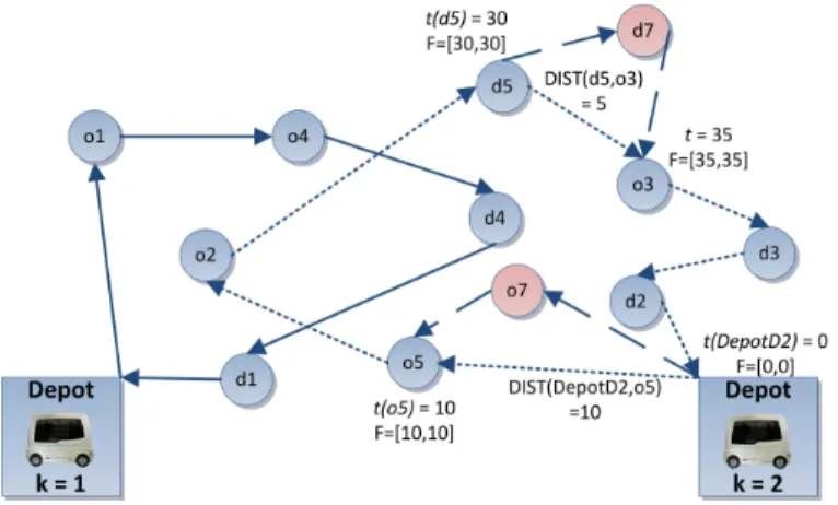
For instance, we consider a fleet of 2 vehicles with two schedules made by a first resolution of the DARP minimizing the total distance. The date of each service time has already given to the users. Once these dates are created, the system has to reduce the time windows to 0 like in the Figure 3. While the vehicles are not already left from the depots, the system needs to integrate one more demand in a second resolution process. Then, each new demand such as (o6,d6) will not be able to be inserted. Indeed, for the origin node we have: t(DepotD2)+ DIST (DepotD2, o5) = t(o5) which make the insertion of o6 impossible.
One more time, the INSER(i, Γ ) values may be used in order to set the service time without to have the problem above. The service time may be calculated
once the process have inserted the virtual demands D-V and the real demands D-R.
Fig. 3. New insertions after the first set of service times
The previous section shows the way to anticipate the future demands D-V . These demands are related to a dynamic context. Note again that our greedy algorithm is easily adaptable to this context. More specifically, the technique does not change unlike the state of each route. The first node is not a depot node anymore but a dynamic node related to the vehicle’s location. The entire constraint propagation process is applied on these new routes. A simulation will be necessary to evaluate the anticipation of the future demands including in the dynamic context.
8
Computational Experiments
In this section, we study the behavior of our Insertability measure used in the resolution of Dial-a-Ride instances. The algorithms were implemented in C++ and compiled with GCC 4.2. In [15], we solve the [4]’s instances by our greedy insertion algorithm based on constraint propagation. We obtained good results in the majority of instances, but, only 1% of the replications gave us a feasible solution on the tenth instance (R10a). The CPU time was smallest or equal to the best times in the literature; we do not work on this feature for this experiment.
8.1 First experimentation: the optimization of the selection of the demand to insert
INSER used in the selection of a demand We note by RDARP the rate of 100 replications which give us a feasible solution obtained by using the solution of [15]. Here, the selection of the demand is based on the lowest number of cars
which are able to accept it. RDARP
Rob is the rate obtained with the same process except that each demand is selected at each iteration by the lowest Insertability value INSER.
The Insertability measure is already efficient once it’s used in the selection of the demands to insert. The rate obtained for the pr08, pr09, pr10 and pr19 are clearly more interesting as shown in table 1 (e.g. for the instance pr08, the rate increases by 56% to 91% of success).
Inst. RDARP RDARPRob
pr01 99 100 pr02 100 100 pr03 97 100 pr04 100 100 pr05 100 100 pr06 100 100 pr07 90 96 pr08 56 91 pr09 18 21 pr10 1 7 pr11 100 100 pr12 100 100 pr13 99 100 pr14 100 100 pr15 100 100 pr16 100 100 pr17 98 100 pr18 99 100 pr19 64 99 pr20 43 56 Av. 83,2 88.5 Table 1. RDARP Vs RDARP Rob
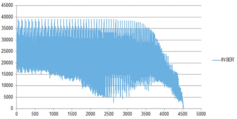
INSER behaviour Each time a replication cannot integrate all the request, the INSER value of the demands not inserted has to be null. In Figure 4, while the resolution process applied to the R10a instance, we note the evolution of more than 4500 INSER’s demands not inserted. The technique used is the second approach selecting the demand by the smallest Insertability. The values noted are from a failed replication.
One can observe big gaps between the different INSER until the 4000 first values. After that, for the remaining requests, the Insertability values decrease strongly because the routes begin to be not flexible. Between the 2500th and the 3500th, for some demands, the values are very low at the beginning just before increasing strongly. This is explained by the fact the process inserts the demand with the lowest INSER but their insertion do not make a big impact on the other
Fig. 4. INSER values on the not inserted demands
demands not inserted. This impact is related to the Optimization Insertability Problem studied below.
8.2 Second experimentation: the optimization of the insertion parameters
In a second experimentation, we compare the [15]’s approach and another algo-rithm based on the optimization of the parameters (x,y,k). The selection of the re-quest to insert is the same for both solutions. For the second one, once a demand i0 is selected, we maximize the sumPi∈D1 −i0INSER(i, Inserted (Γ, i0, k, x, y))
in order the find the best parameter (x,y,k) which will integrate i0in the route k. We do not optimize Mini∈D1 −i0INSER(i, Inserted (Γ, i0, k, x, y)) because we
create instances especially with a set D too large for inserting all the requests. Therefore, the demand with the smallest value INSER for a given parameters (x,y,k) could never be integrated into the routes.
The two algorithms were applied to five sets of 5 randomly generated in-stances. All the instances have their time constraints related to the interval [0;400] and all the load was unit. We set by eF (o) and eF (d)the amplitude of the time windows at the origin and the destination given by the users, respectively. The other parameters are given in table 2.
K eF (o)eF (d) ∆ CAP
10 35 10 ∞ 10 Table 2. Parameters’ instances
We generate 5 different sets of 5 instances with a variation of the number of demands |D|. We set by TInsert and by TInsertRob the demand inserted’s rate
the first resolution and the second technique, respectively. Finally, GapInsert is the gap in percentage between each rate. Its calculation is given by GapInsert= 100.(TInsertRob− TInsert)/TInsert. We launched 100 replications of each technique
on the 5 sets. The results are provided by the table 3.
|D| 50 75 100 150 200 TInsert 100 93.2 78.9 64.2 52.6
TInsertRob 100 96.8 85.3 66.4 54.1
GapInsert 0 3.86 8.11 3.43 2.81 Table 3. Gap between the INSERT rates
In future work, we could integrate the usual performance criterion (like the total distances) in the P erf value in order to choose each best insertion parame-ters. Here, we are just taken into account the INSER values in order to integrate the most requests possible. The results show us that the larger of |D| defines if the system needs to optimize the Insertability measure. For |D| = 50, all the requests are able to be inserted easily, so, the INSER values does not have any interest. When the set is composed of 100 demands, we obtained a GapInsert of 8,11% meaning there are more than 8% more requests inserted by the second approach.
For this set of instance, we also tried to integrate a new feature in our algo-rithm: we’ve added the ability to exclude a request if the impact of one insertion involving a significant drop of the general Insertability’s demands from D1 − i0. Before that, we study the threshold which limits the variation of Insertability.
i0is excluded if P
i∈D1 −i0(INSER(i, Γ ) − INSER(i, Inserted (Γ, i0, k, x, y)))
> ξ is true with ξ a threshold. The calculation of the threshold is not easy. In the figure 8.2, we report Variation which is the difference IN SERav − IN SERap with INSERav and INSERap the valuesP
i∈D1 −i0INSER(i, Γ ) and
P
i∈D1 −i0INSER(i, Inserted (Γ, i0, k, x, y)), respectively. This figure shows us that
the threshold ξ have to be calculated dynamically according to the average of INSER.
We used this type of dynamic threshold for the third set of instances with 100 demands. We exclude an request if the current ξ is exceeded, and only this feature is added in the second approach. We obtained a gain of 1,3% in average (from 85,3% to 86,6%) meaning approximately one more demand is able to be inserted.
Fig. 5. Variation of the Insertability values between each insertion
9
Conclusion
The Dial-a-Ride Problem is one of the transport problems with the highest number of hard constraints like time windows. The insertion techniques are able to obtain a good solution in a reasonable time. Their adaptability to a dynamic context is easy but a lack of robustness could appear once the goal is to integrate requests as much as possible.
We have introduced a way to measure the impact of each insertion on the other demands not inserted. This Insertability measure could be used in order to exclude a demand, to select a demand to insert and also to calculate the best insertion parameters. This value, named INSER, leads to a large amount of work opportunities. We have introduced a simple way to make the model of the future demands, and how to adapt our greedy insertion algorithm based on the constraint propagation to the dynamic context. In future work, we will develop a simulation which is necessary to show the efficiency of the demands anticipation. The final goal will be to adapt these techniques to a real case.
Acknowledgment
This work was founded by the French National Research Agency, the European Commission (Feder funds) and the Region Auvergne in the Framework of the LabEx IMobS3.
References
1. A. Attanasio, J.-F. Cordeau, G. Ghiani, G. Laporte, Parallel Tabu search heuristics for the dynamic multi-vehicle dial-a-ride problem, Parallel Computing, Volume 30, Issue 3, 2004, Pages 377-387.
2. L. Coslovich, R. Pesenti, W. Ukovich, A two-phase insertion technique of unexpected customers for a dynamic dial-a-ride problem, European Journal of Operational Re-search, Vol. 175, Issue 3, 16 December 2006, Pages 1605-1615.
3. R. Chevrier, P. Canalda, P. Chatonnay, D. Josselin, Comparison of three algorithms for solving the convergent demand responsive transportation problem, 2006, Intel-ligent Transportation Systems, Toronto, Canada, 1096-1101.
4. J.-F. Cordeau, G. Laporte, A tabu search heuristic algorithm for the static multi-vehicle dial-a-ride problem, 2003, Transportation Research B 37, 579-594.
5. J-F Cordeau, A Branch-and-cut Algorithm for the Dial-a-Ride, 2006, Operation Research. Vol, 54, 573-586.
6. J.F. Cordeau, G. Laporte, The dial-a-ride problem: models and algorithms, 2007, Annals of Operations Research,153(1):29-46.
7. J.F. Ehmke, Integration of Information and Optimization Models for Routing in City Logistics, 2012, International Series in Operations Research and Management Science, Vol 177. Book.
8. M. Gendreau, J.Y. Potvin, Dynamic vehicle routing and dispatching. In: T.G. Crainic, G. Laporte (Eds.), Fleet Management and Logistics, 1998, pp. 115126. 9. K. Menger, Das botenproblem, 1932, Ergebnisse eines mathematischenkolloquiums
2, 11-12.
10. H. Psaraftis, An exact algorithm for the single vehicle many-to-many dial-a-ride problem with time windows, 1983, Transportation Science 17, 351-357.
11. S.N. Parragh, K.F. Doerner, R.F. Hartl, Variable neighborhood search for the dial-a-ride problem, 2010, Computers & Operations Research, 37, 1129-1138.
12. P. Healy, R. Moll, A new extension of local search applied to the dial-a-ride prob-lem, 1995, European Journal of Operational Research 83, 83-104.
13. H. Psaraftis, N. Wilson, J. Jaw, A. Odoni, A heuristic algorithm for the multi-vehicle many-to-many advance request dial-a-ride problem, 1986, Transportation Research B 20B, 243-257.
14. O. Madsen, H. Ravn, J. Rygaard, A heuristic algorithm for the a dial-a-ride prob-lem with time windows, multiple capacities, and multiple objectives, 1995, Annals of Operations Research 60, 193-208.
15. S. Deleplanque, A. Quilliot, Constraint Propagation for the Dial-a-Ride Problem with Split Loads, 2013, Recent Advances in Computational Optimization. Studies in Computational Intelligence, Vol. 470, Springer, 31-50.