The Accuracy of Radar Estimates of Ice Terminal Fall Speed from Vertically Pointing Doppler Radar Measurements

HAL Id: hal-00598735

https://hal.archives-ouvertes.fr/hal-00598735

Submitted on 22 Nov 2020

HAL is a multi-disciplinary open access

archive for the deposit and dissemination of

sci-entific research documents, whether they are

pub-lished or not. The documents may come from

teaching and research institutions in France or

abroad, or from public or private research centers.

L’archive ouverte pluridisciplinaire HAL, est

destinée au dépôt et à la diffusion de documents

scientifiques de niveau recherche, publiés ou non,

émanant des établissements d’enseignement et de

recherche français ou étrangers, des laboratoires

publics ou privés.

Speed from Vertically Pointing Doppler Radar

Measurements

Alain Protat, Christopher R. Williams

To cite this version:

Alain Protat, Christopher R. Williams. The Accuracy of Radar Estimates of Ice Terminal Fall Speed

from Vertically Pointing Doppler Radar Measurements. Journal of Applied Meteorology and

Clima-tology, American Meteorological Society, 2011, 50 (10), pp.2120-2138. �10.1175/JAMC-D-10-05031.1�.

�hal-00598735�

The Accuracy of Radar Estimates of Ice Terminal Fall Speed from Vertically

Pointing Doppler Radar Measurements

ALAINPROTAT

Centre for Australian Weather and Climate Research, Melbourne, Victoria, Australia, and Laboratoire Atmosphe`re, Milieux, Observations Spatiales, Guyancourt, France

CHRISTOPHERR. WILLIAMS

Cooperative Institute for Research in Environmental Science, Boulder, Colorado (Manuscript received 17 December 2010, in final form 19 May 2011)

ABSTRACT

Doppler radar measurements at different frequencies (50 and 2835 MHz) are used to characterize the terminal fall speed of hydrometeors and the vertical air motion in tropical ice clouds and to evaluate statistical methods for retrieving these two parameters using a single vertically pointing cloud radar. For the observed vertical air motions, it is found that the mean vertical air velocity in ice clouds is small on average, as is assumed in terminal fall speed retrieval methods. The mean vertical air motions are slightly negative (downdraft) between the melting layer (5-km height) and 6.3-km height, and positive (updraft) above this altitude, with two peaks of 6 and 7 cm s21_{at 7.7- and 9.7-km height. For the retrieved hydrometeor terminal}

fall speeds, it is found that the variability of terminal fall speeds within narrow reflectivity ranges is typically within the acceptable uncertainties for using terminal fall speeds in ice cloud microphysical retrievals. This study also evaluates the performance of previously published statistical methods of separating terminal fall speed and vertical air velocity from vertically pointing Doppler radar measurements using the 50-/2835-MHz radar retrievals as a reference. It is found that the variability of the terminal fall speed–radar reflectivity relationship (Vt–Ze) is large in ice clouds and cannot be parameterized accurately with a single relationship. A

well-defined linear relationship is found between the two coefficients of a power-law Vt–Zerelationship, but

a more accurate microphysical retrieval is obtained using Doppler velocity measurements to better constrain the Vt–Zerelationship for each cloud. When comparing the different statistical methods to the reference, the

distribution of terminal fall speed residual is wide, with most residuals being in the 630–40 cm s21range about the mean. The typical mean residual ranged from 15 to 20 cm s21, with different methods having mean residuals of ,10 cm s21at some heights, but not at the same heights for all methods. The so-called Vt–Ze

technique was the most accurate above 9-km height, and the running-mean technique outperformed the other techniques below 9-km height. Sensitivity tests of the running-mean technique indicate that the 20-min av-erage is the best trade-off for the type of ice clouds considered in this analysis. A new technique is proposed that incorporates simple averages of Doppler velocity for each (Ze, H) couple in a given cloud. This technique,

referred to as DOP–Ze–H, was found to outperform the three other methods at most heights, with a mean

terminal fall residual of ,10 cm s21_{at all heights. This error magnitude is compatible with the use of such}

retrieved terminal fall speeds for the retrieval of microphysical properties.

1. Introduction

Ice clouds are crucial components of the earth’s ra-diative balance. Properly representing ice clouds in numerical models is a major challenge because cloud

parameterizations in climate models represent the largest source of spread among future climate projections (e.g., Bony et al. 2006; Dufresne and Bony 2008; Sanderson et al. 2008; Mitchell et al. 2008). Representing clouds in models also significantly affects the quality of weather forecasts (e.g., Jakob 2002), especially where observations are sparse. Large-spatial-domain models are increasing in complexity, often embedding several smaller-spatial-scale models to capture complex processes, making the evaluation and improvement of models difficult (Jakob

Corresponding author address: Alain Protat, Laboratoire At-mosphe`re, Milieux, Observations Spatiales (LATMOS), 11, Bou-levard d’Alembert, 78280 Guyancourt, France.

E-mail: alain.protat@latmos.ispl.fr DOI: 10.1175/JAMC-D-10-05031.1 Ó 2011 American Meteorological Society

2003). One particularly challenging aspect for models is correctly representing the cloud life cycle, which, in reality, is the result of complex microphysical processes, radiative processes, dynamic processes, advection pro-cesses, and the interactions between these processes.

Two crucial cloud parameters for the ice cloud life cycle are the terminal fall speed of the hydrometeors and the ambient air motion that advect the hydrome-teors through its environment. A recent climate-model sensitivity study showed that ice cloud terminal fall speed had the second largest model impact behind en-trainment rate in deep convection (Sanderson et al. 2008). Decreasing the ice cloud terminal fall speed in Sanderson et al. (2008) was related to an increase in both cirrus cloud cover and longwave cloud forcing. In a similar way, Jakob (2002) found that changes in the ice fall speed in the European Centre for Medium-Range Weather Forecasts model led to large changes in cirrus cloud ice water path and longwave cloud forcing. Get-ting the sedimentation of ice correct in models appears to be an important problem as well as an opportunity for improvement.

There are several ice cloud hydrometeor sedimenta-tion parameterizasedimenta-tions currently used in climate models (e.g., Heymsfield and Donner 1990; Sundqvist 2002; Wilson and Ballard 1999; Rotstayn 1997; Morrison and Gettelman 2008). Combining the sensitivity of models to ice cloud terminal fall speed parameterization with the variety of ice cloud sedimentation parameterizations, the previously discussed large spread in climate projections may be due to how clouds are represented in models. It is believed that observations of ice clouds and their statis-tical properties, which include time–height variability and relationship to the large-scale environment, will help to model ice cloud sedimentation parameterization. Ob-servations of ice particles from in situ aircraft and labo-ratory measurements have been used to characterize the terminal fall speed of different ice particle types, with the most recent results being presented in Heymsfield and Westbrook (2010). Although there has been work done to document the transition from the terminal fall speed of individual particles to that of an ensemble of particles found in a model or a radar volume (e.g., Heymsfield et al. 2007), there is still a need for a better character-ization of the vertical variability (or variability as a func-tion of ambient temperature). Ground-based vertically pointing radars are ideal for studying the temporal and vertical variability of cloud systems.

Deng and Mace (2008) recently produced a statistical characterization of the properties of terminal fall velocity in cirrus clouds from long-term ground-based observa-tions from the U.S. Department of Energy’s Atmospheric Radiation Measurement Program (ARM; Ackerman and

Stokes 2003) at midlatitudes and in the tropics. They developed a robust relationship among mass-weighted terminal fall speed, ice water content, and ambient tem-perature, resulting in a parameterization for cirrus in large-scale models. In the study of Deng and Mace (2008) though, the retrieved terminal fall speed is not directly related to the observed cloud radar Doppler velocity but is derived from a parameterization of particle fall velocity as a function of maximum particle diameter (Heymsfield and Iaquinta 2000) with an assumption on particle habit.

Vertically pointing Doppler cloud radars can in principle provide information about the reflectivity-weighted terminal fall speed of ice cloud hydrometeors and the ambient air motion. One difficulty with vertically pointing cloud radars, however, is that the Doppler measurement is the sum of the reflectivity-weighted ter-minal fall speed and the vertical air velocity, which must be separated using retrieval methods. Statistical methods (which will be reviewed in section 4) have been proposed in the literature to separate the two vertical motions when using a single cloud radar (e.g., Orr and Kropfli 1999; Matrosov et al. 2002; Protat et al. 2003; Delanoe¨ et al. 2007; Plana-Fattori et al. 2010), but these methods have not been thoroughly validated using an independent and presumably more accurate vertical air motion estimate. In situ aircraft observations would appear as attractive validation datasets, but these measurements also require some assumptions (e.g., zero mean vertical air motion for a given level flight path segment) that prevent an independent validation of previously proposed statis-tical methods.

In this paper, recent observations from multiple ver-tically pointing radars collected near Darwin, Northern Territory, Australia (described in section 2), are processed with innovative techniques generating simultaneous in-dependent estimates of reflectivity-weighted terminal fall velocities (which will be referred to as ‘‘terminal fall velocity’’ throughout the paper) and vertical air mo-tions within ice clouds (section 3). Previously proposed statistical methods to isolate the vertical air motion from single-frequency cloud radar observations are presented in section 4, and the new Darwin observations are used to characterize the errors of these statistical retrieval methods (section 5). A new method is also proposed in section 6, which is found to outperform statistically the existing statistical methods. Conclusions are given in section 7.

2. The radar observations around Darwin

In the 1980s and early 1990s, the National Oceanic and Atmospheric Administration (NOAA) developed

wind profilers operating at 50 and 915 MHz to study the tropospheric wind motions associated with El Nin˜o (Carter et al. 1995). The 50-MHz profiler can directly observe the vertical air motion from Bragg scattering from turbulent inhomogeneities in refractive index caused by gradients in humidity and temperature throughout the troposphere (Balsley and Gage 1982). The 50-MHz wind profiler can also resolve the Rayleigh scattering processes due to hydrometeors (Fukao et al. 1985). Simultaneously observing the ambient air mo-tion and hydrometeor momo-tion enables the 50-MHz profiler to be used in studying the vertical structure of precipitating cloud systems (Wakasugi et al. 1986). The 920-MHz profiler predominantly observes the Rayleigh scattering from the hydrometeors in the radar pulse volume and has been used in several tropical precipi-tation research projects (Rogers et al. 1993a,b; Gage et al. 1994, 1996; Ecklund et al. 1995; Williams et al. 1995). When the radar beam is pointed off vertical, these radars are called wind profilers and can estimate the horizontal wind in ‘‘clear air’’ using the Bragg scat-tering feature (Gage and Gossard 2003). NOAA also developed a profiler operating at 2835 MHz (S band) to study the vertical structure and the evolution of precipitating cloud systems using short dwell periods (;10–30 s) (Ecklund et al. 1999).

The observations used in this study come from radars operating at the three frequencies discussed previously and have been collected as part of the Tropical Warm Pool–International Cloud Experiment (TWP-ICE; May et al. 2008). As discussed in May et al. (2008), the Dar-win area hosts an extensive ground-based observational network that includes long-term components as well as instruments deployed specifically for campaigns. Long-term components included Australian Bureau of Mete-orology instrumentation such as scanning Doppler radars and radar wind profilers, as well as the U.S. Department of Energy Atmospheric Cloud and Radiation Facility (ACRF) site (Ackerman and Stokes 2003).

Of particular interest to this study are the three wind profilers operating at three frequencies: very high fre-quency (VHF) (50 MHz; Vincent et al. 1998), UHF (920 MHz; Carter et al. 1995), and S-band (2835 MHz; Ecklund et al. 1999). This profiler site was also hosting a Joss–Waldvogel disdrometer and two tipping-bucket rain gauges. The 920- and 2835-MHz radars have been intercalibrated and calibrated against the disdrometer measurements. This profiler site is located 8 km south-east of the Darwin ACRF site, which hosts (among other instruments) a 35-GHz cloud radar (Moran et al. 1998) and a cloud lidar (Clothiaux et al. 2000) for the characterization of the vertical distribution of cloud properties.

3. Vertical air velocity and terminal fall velocity retrieval using 50-/920-MHz Doppler radar spectra and Doppler S-band radar measurements As discussed in the previous section, both Rayleigh and Bragg scattering processes can simultaneously be resolved in 50-MHz profiler Doppler velocity power spectra. The two scattering processes will appear in two regions of the Doppler velocity spectra with the Rayleigh scattering from hydrometeors always falling downward relative to the Bragg scattering. Figure 1 illustrates the two scattering processes using a vertical profile of Doppler velocity power spectra from the Darwin 50-MHz profiler (Fig. 1a) and 920-MHz profiler (Fig. 1b) during a con-vective event at 0000 UTC on 20 January 2006. The color scales show relative backscattered power scaled to reflectivity spectral density [dBZ (m s21)21]. In Fig. 1a, the two dominant peaks between 2 and 5 km represent the vertical air motion (ranging between 2 m s21 down-ward at 3.5 km and 6 m s21upward at 5 km) and the hydrometeor motion that is about 6 m s21 downward relative to the vertical air motion. In Fig. 1b, the 920-MHz profiler is only sensitive to the backscattered energy of the hydrometeors and thus shows the hydrometeor mo-tion, which is the combination of the hydrometeor fall speed and the vertical air motion. The retrieved vertical air motions are displayed in Fig. 1b to show the relative position of the 920-MHz profiler hydrometeor motion.

Although our eyes can identify the two scattering processes in the 50-MHz observations (Fig. 1a), a dual-frequency technique was developed to help to isolate the Bragg scattering signal in the 50-MHz profiler Doppler velocity power spectra (C. R. Williams 2011, unpublished manuscript). To simply describe the dual-frequency tech-nique, the 920-MHz profiler Doppler velocity power spectra are used to mask out the hydrometeor signal in the 50-MHz profiler spectra to better highlight the ver-tical air motion signal. A dominant-peak-picking routine is applied to the filtered 50-MHz profiler spectra identi-fying the vertical air motion, and the first three moments are calculated: signal-to-noise ratio (SNR), mean radial velocity, and spectrum width. The mean radial velocity and spectrum width are shown in Figs. 1a and 1b. When there is no 920-MHz signal but still a 50-MHz signal, it is assumed in the method that the 50-MHz signal is due to Bragg scattering, which allows for the retrieval of vertical air motion from the 50-MHz signal.

The 920- and 50-MHz wind profilers are used for op-erational weather forecasting and are designed to mea-sure the winds from 200 m to 10 km in near–real time. Thus, the 920-MHz profiler was not designed to observe ice clouds above the freezing level near 6 km. There-fore, during TWP-ICE a 2835-MHz vertically pointing

radar (S-band radar) was installed next to the 920- and 50-MHz profilers. The S-band radar was absolutely calibrated with a surface Joss–Waldvogel disdrometer, and the reflectivity and mean Doppler velocity for the 20 January 2006 event are shown in Figs. 2a,c, with the same color scale as the same measurements from the 920-MHz profiler (Figs. 2b and 2d, respectively). Note that the S-band radar observed higher heights than the simultaneous 920-MHz profiler (Fig. 2a), owing to better sensitivity, but that the reflectivity and Doppler veloci-ties are very similar in the common sample volume. Because the S-band profiler is more sensitive than the 920-MHz profiler, it has been chosen in this study to derive the terminal fall speed by subtracting the vertical air motions derived from the 50–920-MHz pair to the S-band Doppler velocities. This allows for terminal fall speed retrievals at higher heights than when using the 920-MHz profiler data.

One key parameter in evaluating the cloud radar statistical retrievals of terminal fall speed and vertical air

velocity will be the uncertainty of both the dual-frequency profiler vertical air motions and the S-band radar radial velocities. Worker C. R. Williams (2011, unpublished manuscript) shows using Monte Carlo sim-ulations that radial velocity uncertainties are dependent on the measured SNR and spectrum width. The errors overall primarily increase with spectrum width. When reaching the lowest SNRs, however, at cloud edges for instance, the errors will increase primarily because of low SNR. For the ice clouds observed in this study, the vertical air motion uncertainty ranged from about 0.02 to 0.20 m s21 _{typically, and the S-band radar radial}

velocity uncertainties ranged from as low as 0.005 to 0.05 m s21typically, except at ice cloud tops (charac-terized by small SNR) where uncertainties can reach 0.1 m s21. Although the details of estimating the radial velocity uncertainty are given in C. R. Williams (2011, unpublished manuscript), the uncertainties for differ-ent ice cloud regimes iddiffer-entified in this study will be presented in section 4.

FIG. 1. Radial velocity power spectra collected near Darwin during TWP-ICE at 0000 UTC 20 Jan 2006. The vertical axis is height (km), and the horizontal axis is radial velocity with more downward motions to the right of zero velocity. (a) Observations from a 50-MHz profiler; the dual-frequency technique radial velocity peak is identified with a black asterisk, the spectrum width is shown with a black horizontal line, and the start and end integration points for the moment calculations are shown with red times signs. (b) Observations from a collocated 920-MHz profiler with the asterisks, horizontal lines, and times signs that are shown in (a) also shown for clarity.

FIG. 2. Illustration of the dual-frequency radar retrieval of terminal fall speed and vertical air velocity on the 23 Jan 2006 stratiform precipitation case over Darwin. (a) S-band radar reflectivity (dBZ), (b) 920-MHz radar reflectivity (dBZ), (c) S-band radar radial velocity (positive is upward; m s21_{), (d) 920-MHz radar radial velocity (positive is}

upward; m s21_{), (e) vertical air velocity retrieved using the 920/50-MHz radar combination (positive is upward;}

m s21_{), (f) retrieved terminal fall velocity using S-band radar radial velocity and retrieved 920/50-MHz radar}

combination vertical air velocity (m s21_{), (g) vertical air velocity retrieval uncertainty (m s}21_{), and (h) S-band radar}

radial velocity uncertainty (m s21_{). Note that the terminal fall velocity uncertainty is very close to the vertical air}

velocity uncertainty and is therefore not displayed here.

To illustrate the multiple steps needed to retrieve the ice cloud terminal fall speeds from multiple radar ob-servations, Fig. 2 shows observations and retrievals of a stratiform precipitation case that passed over the Dar-win profiler site on 23 January 2006 during the active monsoon phase of the TWP-ICE experiment (May et al. 2008). The S-band profiler reflectivity and radial velocity are shown in Figs. 2a and 2c, respectively. Typical signatures of stratiform precipitation are found, with a well-marked transition between the ice phase and the liquid phase, separated by the so-called radar bright band just below the melting layer (or 08C isotherm alti-tude). The ice phase is characterized by much smaller downward radial velocities than in the liquid phase, which is predominantly due to the terminal fall speed contri-bution. Cloud tops up to 17-km height are measured for this case with the S-band radar, but the 920-MHz profiler only observed up to 10 km (Fig. 2b). The vertical air velocity retrieved from the dual-frequency spectra tech-nique is shown in Fig. 2e. It is striking to see how variable the vertical air motion field is even in stratiform pre-cipitation, with well-defined updraft–downdraft struc-tures of 60.5–0.8 m s21. The S-band radar radial velocity uncertainty is shown in Fig. 2h and is less than 0.02 m s21 in most of the ice part and increases near the ice cloud edges (up to 0.05 m s21), showing the increase of errors only for lowest SNRs (C. R. Williams 2011, unpublished manuscript). Figure 2f shows the ice cloud and liquid precipitation terminal fall velocity estimated by sub-tracting the vertical air motion from the S-band radial velocity. Typical values from 29 to 25 m s21are found in the liquid phase, and the ice cloud terminal fall velocities are typical (from 22 to 20.4 m s21) and will be discussed further in the following sections. The estimated vertical air velocity uncertainty is displayed in Fig. 2g. Note that because of smaller errors on S-band radar radial velocity, the resulting error on terminal fall speed is primarily due to the errors on vertical air velocity. In ice phase, these errors rarely exceed 0.15 m s21but can be larger in liquid phase (up to 0.25 m s21). These errors are primarily due to regions of high spectrum width (not shown), as also dis-cussed in C. R. Williams (2011, unpublished manuscript).

4. Terminal fall speed retrieval using Doppler cloud radar measurements

Doppler cloud radars do not measure the reflectivity-weighted terminal fall velocity of ice particles directly. The Doppler radar measurement is the sum of the reflectivity-weighted velocity of the ice particles Vtand

the vertical air motion w. All of the following techniques aim to separate these two contributions by applying dif-ferent assumptions to cloud radar observations. Recall

that these methods have not been evaluated and com-pared with any kind of ground truth so far, yet they have been applied to Doppler cloud radar measurements to estimate the terminal fall speeds so as to retrieve micro-physical and radiative properties of ice clouds.

a. The Vt–Zetechnique

A first statistical approach to estimate Vt(hereinafter

referred to as the Vt–Zetechnique) was used to study

frontal cyclones and nonprecipitating ice clouds (i.e., clouds that do not produce precipitation at the ground; Orr and Kropfli 1999; Protat et al. 2003; Delanoe¨ et al. 2007). The method consists of developing for each cloud under study a power-law relationship between Doppler velocity and radar reflectivity:

V_D 5aZ_eb(m s21), (1) where Zeis radar reflectivity expressed in millimeters

to the sixth power per cubic meter and a and b are the coefficients of VD–Ze relationship obtained by linear

regression.

Within nonprecipitating clouds, the vertical air mo-tions are generally small, in contrast to convective sys-tems. In any case, however, the vertical air motions are not negligible with respect to the ice particle terminal fall speed. For a long dwell period, however, the mean vertical air motions should vanish (or average to zero) with respect to the mean terminal fall speed, which is much less fluctuating. Under this approximation, the use of Eq. (1) allows directly for the retrieval of terminal fall speed. Following this approach, the scatter around the fitted curve is attributed to vertical air-motion fluctua-tions and not to fluctuafluctua-tions in terminal fall velocities.

The implicit assumption of this approach is that the cloud microphysical characteristics do not change within the cloud (the nature of the Vt–Zerelationship is the

same everywhere in the cloud). It is clear that this ap-proach is not perfect; in particular, it is expected that the Vt–Zerelationship will change in the vertical direction as

the dominant particle habit and particle density change in response to microphysical growth processes. Despite this possible shortcoming, however, the potential ad-vantage of this method is that the Vt–Zerelationship is

not fixed once for all clouds [e.g., as is the case implicitly in Deng and Mace (2006)] but is retrieved for each cloud from the Doppler velocity–reflectivity measurements. The importance of using adaptive Vt–Zerelationships

will be discussed and illustrated further in section 5. b. The Vt–Ze–H technique

To overcome the potential problem of the Vt–Ze

re-lationship changing with height, Plana-Fattori et al. (2010)

proposed a formulation that includes the height H as an additional input parameter. The mathematical relation-ship among Vt, Ze, and H is assumed to have the form

V_D5a₁₁Ha12_Z(b111b12H) _{(m s}21_{). (2)}

Apart from specifying the height, the Vt–Ze–H

technique makes the same assumptions as the Vt–Ze

technique. The mathematical formulation of the de-pendency with height H has been chosen for the sake of simplicity because the parameters can easily be solved using a simple least squares fit, as for the Vt–Ze

tech-nique. It must be noted, however, that the use of a pre-scribed mathematical shape may introduce errors that have not been characterized so far. This will be studied further in section 5. Note also that, when applied to millimeter-wavelength radar observations, the Vt–Ze

and Vt–Ze–H techniques are sensitive to non-Rayleigh

scattering, which will tend to modify the relationship between terminal fall speed and reflectivity for the larger reflectivities.

c. The running-mean technique

A simple alternative approach to the two statistical methods described previously has been proposed by Matrosov et al. (2002) and estimates the terminal fall velocities by averaging 20 min of radar observations. This technique assumes that the averaged residual ver-tical air motion is negligible relative to the averaged terminal fall speed. This approach has been refined by using 20-min running means at the full resolution of the radar measurements (Delanoe¨ et al. 2007), allowing for some small-scale variability due to possible small-scale changes in the cloud microphysical characteristics to be retained. This method will be referred to as the ‘‘running mean’’ technique in the following.

The running-mean technique has advantages over the statistical methods by assuming ‘‘steady’’ microphysics for a shorter time scale of 20 min horizontally and avoiding any assumption in the vertical direction. When applied to millimeter-wavelength radar observations, it is not expected to be sensitive to non-Rayleigh scatter-ing because it does not rely on a relationship between reflectivity and fall speed. One possible drawback, though, is that the vertical air motion could be less ac-curately filtered out by using this relatively small time span (our experience is that this technique can even produce upward fall speeds in the upper part of the ice clouds where fall speeds are typically small). Another potential problem with this method is that a 20-min averaging window is an arbitrary duration that has never been evaluated thoroughly. Sensitivity tests will be presented in section 6b.

5. The statistical properties of terminal fall speed and vertical air velocity

Using multiple-frequency radars to identify and quan-tify the vertical air motion and ice cloud terminal fall velocity as presented in section 3 is a more direct way to isolate the two velocities than the single-frequency radar techniques presented in section 4. This section uses the multiple-frequency radar-derived vertical air motion and terminal fall speeds to characterize the statistical prop-erties of the single radar techniques in tropical ice clouds. This analysis includes 20 case studies collected during the 2005/06 wet season over Darwin. The dual-frequency vertical air motion w and S-band-radar-retrieved termi-nal fall speed Vtwere available for all 20 cases. All

pe-riods of convective rain were systematically discarded, because the statistical methods of section 4 cannot be applied to those cases. Table 1 provides more information about the retained cases, time intervals used, and type of ice clouds sampled. A simple visual classification divided the cases into four categories: stratiform precipitating systems, thick anvil clouds produced by deep convection, cirrus clouds (base and top higher than 7–8 km), and al-tostratus clouds (base and top lower than 7–8 km). This dataset does not include high-altitude cirrus clouds or the upper part of stratiform precipitation and thick anvil clouds, because the sensitivity of the 50-MHz radar does not allow for the retrieval of vertical air motions at alti-tudes greater than 10–11 km.

TABLE1. The cases processed for this study: nine stratiform precipitation cases (36.2 h of observations), six thick nonpreci-pitating anvils (15.2 h of observations), four cirrus clouds (8.8 h), and one altostratus cloud (2.2 h).

Date Hours (decimal)

Type of ice cloud sampled

13 Nov 2005 17.9–22.0 Thick nonprecipitating anvil

14 Nov 2005 7.0–10.0 Thick nonprecipitating anvil

17 Nov 2005 15.0–19.0 Stratiform precipitation

20 Nov 2005 4.5–10.0 Stratiform precipitation

20 Nov 2005 12.0–14.2 Altostratus

20 Nov 2005 14.7–20.0 Stratiform precipitation

21 Nov 2005 22.0–24.0 Thick nonprecipitating anvil

22 Nov 2005 0.0–3.0 Thick nonprecipitating anvil

23 Nov 2005 11.0–12.5 Stratiform precipitation

24 Nov 2005 4.0–7.0 Cirrus

25 Nov 2005 7.9–10.0 Cirrus

2 Dec 2005 3.5–6.0 Cirrus

4 Dec 2005 20.0–21.2 Cirrus

4 Dec 2005 21.2–22.6 Stratiform precipitation

4 Dec 2005 22.6–24.0 Thick nonprecipitating anvil

20 Jan 2006 1.0–5.0 Stratiform precipitation

22 Jan 2006 12.0–18.0 Stratiform precipitation

23 Jan 2006 11.0–15.5 Stratiform precipitation

23 Jan 2006 20.0–24.0 Stratiform precipitation

10 Feb 2006 14.3–16.0 Thick nonprecipitating anvil

a. The natural variability of terminal fall speed as a function of reflectivity

A main assumption in the Vt–Zeand Vt–Ze–H

tech-niques is that the variability of terminal fall velocity due to changes in microphysical properties inside a given cloud (dominant particle habit, particle density, cross-sectional area, etc.), which we will refer to as the ‘‘nat-ural’’ variability in what follows, is much smaller than the variability of vertical air velocity for a given value of reflectivity. This terminal fall speed variability as a function of reflectivity due to microphysics has not been investigated from direct measurements of terminal fall speed, however. It has been so far mostly investigated from in situ particle size distribution measurements in tropical ice clouds (e.g., Heymsfield et al. 2007), but these estimates do rely on assumptions about particle habit, density, and fall speed–diameter relationships, which al-lows for this natural variability to be characterized.

The terminal fall speed variability as a function of reflectivity can be estimated using the S-band radar-derived terminal fall speed, the S-band radar reflectivity, and the vertical air velocity from the dual-wavelength observations (see section 3) as the reference and calcu-lating the standard deviation of the terminal fall velocity s_V

t(zj) in each reflectivity bin zjas

s_V t(zj) 5 1 N_p(z_j)

å

where Np(zj) is the number of samples in each

re-flectivity bin, V_t

iis the ith S-band radar-derived terminal

fall speed sample in the reflectivity bin, and V_t

fit is the

terminal fall speed from one of the statistical methods presented in section 4.

The standard deviation of the terminal fall velocity has been calculated for all 20 cases of Table 1 and as an ensemble to provide an estimate of the natural vari-ability from a large number of points and a large variety of ice cloud types. However, different factors contribute to the variance of Vtas a function of Zein addition to the

microphysics component. First, owing to the vertical stratification of air density in the troposphere (decreasing exponentially with height), the same ice particle will not fall at the same terminal fall speed at different heights in the troposphere. To remove this variability that is not related to microphysics, all individual terminal fall speed estimates have been ‘‘referenced’’ to ground level before calculating the standard deviation of Vtas a function of

Ze, using a multiplying correction factor f(H) 5 [r(H)/

r(0)]0.4, where r(H) is air density at altitude H (Foote and Du Toit 1969; Protat et al. 2003). Once this correction is done, the remaining contributions to the variance refer-enced to ground level (denoted as s2

V_t(zj)jG in the

fol-lowing) are the variance due to microphysics s2V_t(zj)jM

(which is what we are trying to characterize) and the variance due to the uncertainty of the terminal fall speed retrieval method s2

V_t(zj)jU(which has been estimated for

each case, as discussed in section 3). The natural vari-ability of terminal fall speed as a function of reflectivity due to microphysics is then finally calculated as

s_V t(zj)jM 5[s 2 V_t(zj)jG2 s 2 V_t(zj)jU] 1/2_{. (4)} This s_V

t(zj)jM term is shown over the [210, 30]

re-flectivity range in Fig. 3, both when all cases are included

FIG. 3. Natural standard deviation of terminal fall speed as a function of S-band radar reflectivity: when all cases of Table 1 are included and terminal fall speeds are referenced to the ground level (solid black line) or taken at their altitude (dotted black line), and for different ice cloud categories: cirrus (blue line), thick anvils (green line), and stratiform precipitation (red line). The dashed line corresponds to the mean terminal fall velocity uncertainty in each radar reflectivity bin.

and when data are split into the three ice cloud cate-gories (thick anvils, stratiform precipitation, and cirrus). First, when all cases are included it is obtained that the natural variability of terminal fall speed referenced to ground level is of about 0.25 m s21(thick black line in Fig. 3)—relatively constant over the reflectivity range. Note that when terminal fall velocities are not refer-enced to ground level the variability is much larger (from 0.30 to 0.40 m s21), which is due to the variation of the density of air as a function of height (Fig. 3). This variability of about 0.25 m s21is relatively small when considering possible changes in dominant particle habits from cloud top to cloud base as a result of microphysical growth processes and corresponding changes in the Vt–Ze

relationship (see, e.g., Heymsfield and Iaquinta 2000; Heymsfield et al. 2007). From Fig. 3 it is also seen that there are some differences between the ice cloud cate-gories: smallest variability in stratiform precipitation (typically 0.15–0.20 m s21), intermediate in thick anvils (0.25 m s21), and much larger in cirrus clouds (from 0.35 up to 0.45 m s21). The s_V

t(zj)jU term (variability

due to the uncertainty of the terminal fall speed re-trieval; dashed line in Fig. 3) has also been estimated and is smaller than the natural variability. This term decreases as a function of reflectivity, ranging from 0.13 (for the lowest reflectivities) to 0.10 (for the largest re-flectivities) m s21.

An important conclusion of this work is that because the natural variability of terminal fall speed in reflec-tivity bins is relatively small, it does validate the idea that there is a tight relationship between terminal fall speed and radar reflectivity in tropical ice clouds [which is the basic assumption of methods such as that pre-sented in section 4a and in Orr and Kropfli (1999); Protat et al. (2003); Delanoe¨ et al. (2007)], at least for the rel-atively optically thick ice clouds included in this analysis. The variability of this relationship from one ice cloud to another has not been evaluated, however. It will be studied in the next section.

Delanoe¨ et al. (2007) presented sensitivity tests of their method for the retrieval of the ice microphysical properties by assuming errors of about 10 cm s21for Vt

(either a Gaussian noise or a bias due to the presence of vertical air motions). These authors showed that the root-mean-square (rms) errors on ice water content and extinction can reach about 15%–30% for ice water content and 45% for visible extinction. It is therefore expected that the natural variability of terminal fall speed will introduce a random component of this same order of magnitude (15%–30% for IWC, 45% for visible extinction) using this type of Doppler radar method. This result also highlights the importance of accurately separating out the terminal fall speed and vertical air

velocity components from the Doppler velocity mea-surements. We will go back to that point in section 6. b. The variability of the terminal fall

speed–reflectivity relationship

In some Doppler radar retrieval methods (e.g., Babb et al. 1999; Deng and Mace 2006), the contribution of terminal fall speed is directly subtracted from the Doppler velocity measurement using a relationship between in-dividual fall speed and maximum dimension of each ice particle (e.g., Heymsfield and Iaquinta 2000; Mitchell 1996) integrated over an assumed ice particle size distri-bution. An ice particle habit, which is considered to be the same inside a given cloud and for all types of ice clouds, needs to be assumed. We can check this hypothesis with our multiple-frequency radar observations.

To do so, a Vt–Zepower-law relationship [i.e., Eq. (1),

but replacing VDby Vt] has been derived for all 20 cases

of Table 1 using the direct terminal fall speed estimates (using the method described in section 3) and the S-band reflectivities. Let us recall that the terminal fall speeds have also been referenced to ground level, as discussed in the previous section. The a and b coefficients of these Vt–Zerelationships have been plotted against each other

in Fig. 4. There are several things to note in this figure. First, it is interesting to see that there is a well-defined relationship between the two coefficients of the Vt–Ze

relationship (at least for the tropical ice clouds included in this analysis). This relationship can be approximated by a linear function (b 5 20.44a 1 0.41). This result is

FIG. 4. The relationship between the a and b coefficients of the V_t5aZb

e relationship [Vt: m s21; Ze: linear units (mm6m23)].

Numbers refer to cases of Table 1, and color code is the same as in Fig. 3, with the addition of the altostratus category in light blue. The coefficients for five particle habit assumptions described in Hong (2007) are shown with the labels COL, ROS, AGG, PLA, and DRO, as defined in the text. The terminal fall speeds are ref-erenced to ground level in this figure.

reminiscent of the study of the coefficients of the power-law relationship between ice particle fall speed and maximum particle dimension y(D) at the scale of in-dividual ice crystals by Matrosov and Heymsfield (2000). When plotting the coefficients of y(D) for the different ice particle habits of Mitchell (1996), they indeed found that the two coefficients were linked as well. This in-teresting property of the Vt–Zerelationship will

proba-bly be useful for further development of ice microphysical retrieval methods using Doppler radar observations, but it is out of the scope of this study.

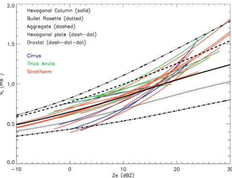
Figure 4 also shows a wide range of a and b values even in the limited tropical ice cloud sample used here, with a ranging from 0.35 to 0.80 and b ranging from 0.01 to 0.26. This is further illustrated in Fig. 5, with all ter-minal fall speeds derived from the cases of Table 1 dis-played as a function of their respective measured radar reflectivity ranges. From Fig. 5, it is found that the maximum differences in terminal fall speed produced by these different relationships in any reflectivity bin do not exceed 0.4 m s21 and are typically of about 0.3 m s21. Although it is obtained from a very different approach, this number is very similar to the natural variability found in the previous section (Fig. 3).

For the sake of comparison, the five sets of (a, b) co-efficients that can be used in the Deng and Mace (2006)

Doppler radar retrieval method [corresponding to five particle habit assumptions described in Hong (2007): hexagonal columns (COL), bullet rosettes (ROS), ag-gregates (AGG), hexagonal plates (PLA), and droxtals (DRO)] are also shown in Fig. 4, as are the corresponding five Vt–Zerelationships in Fig. 5. It is interesting to see

that these five relationships derived from the y(D) of Heymsfield and Iaquinta (2000) and using the radar backscattering coefficients of Hong (2007) for the calcu-lation of the radar backscattering cross section from the assumed ice particle size distribution do bound the measured Vt–Zerelationships for the different ice cloud

types (Fig. 5). This result suggests that the use of these five habits is sufficient to represent the natural variability. It is also observed in Fig. 4, however, that the (a, b) of these five relationships are not all aligned along the pa-rameterized linear relationship between a and b, except for the hexagonal columns and the aggregates (Fig. 4). The fact that the Vt–Zerelationships for hexagonal plates

and bullet rosettes—which are ice particles typically found in thin cirrus clouds that are not included in our analysis—are relatively far from the parameterized re-lationship probably indicates that the parameterized lin-ear relationship between the a and b coefficients should not be used to describe the Vt–Ze relationship in thin

cirrus. Also, assuming the hexagonal column or aggregate

FIG. 5. The variability of the Vt–Zerelationship in ice clouds. Color code is as in Fig. 3. Five

relationships derived using typical particle habits (see text for details) are also given: hexagonal columns (solid), bullet rosettes (dotted), aggregates (dashed), hexagonal plates (dash–dotted), and droxtals (dash–dot–dot). The terminal fall speeds are referenced to ground level in this figure.

habits in Doppler radar methods such as in Deng and Mace (2006) would be appropriate for the cloud types included in our analysis. In examining Fig. 5 again, it is clear, however, that if a single relationship must be as-sumed in retrieval methods then typically the aggregates relationship will tend to produce a general overestimation of fall speed except for reflectivities of larger than 20 dBZ. In contrast, the hexagonal column relationship would be the best trade-off for reflectivities of lower than 20 dBZ but will tend to underestimate terminal fall speed for re-flectivities larger than 20 dBZ. This result also suggests that the use of the statistical terminal fall speed retrieval techniques reviewed in section 4 are probably more ap-propriate (e.g., Matrosov et al. 2002; Delanoe¨ et al. 2007; Plana-Fattori et al. 2010) than the assumption of a single particle habit for any given ice cloud or for all ice clouds. As discussed previously, the accuracy of these techniques has not yet been documented, however. The performance of these terminal fall speed retrieval techniques will therefore be assessed in section 6.

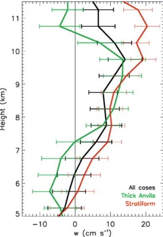
c. The vertical air velocity in tropical ice clouds The combined effect of particle fall speed and in-cloud vertical air velocity is a crucial factor influencing the life cycle of clouds and convection. It is presumed that the long-lived cloud systems are those characterized by sufficiently large upward vertical motions to com-pensate for particle fall speed, allowing for particle growth in ice phase. In this section we examine the mean vertical profiles of vertical air motions for the case studies listed in Table 1 and for different ice cloud cat-egories. Because there are not many cases of altostratus and cirrus clouds, mean vertical profiles of vertical air velocities have been derived only for the thick anvils and stratiform categories, however.

Figure 6 shows the mean vertical profiles of in-cloud vertical air velocity for thick anvils, stratiform, and all cases, as well as the mean uncertainties of vertical air motion at each height. From the uncertainty estimates, it appears that most updraft/downdraft signatures are statistically significant (i.e., the error is smaller than the peak values observed), except maybe the downdraft signature just above the melting layer when all cases are considered. From this figure, it is seen that, when all ice clouds of Table 1 are included, the mean vertical air motions are slightly negative between the melting layer (5-km height) and 6.3-km height and are positive above this altitude, with two peaks of 9 and 14 cm s21at 7.7- and 9.7-km height. The stratiform precipitation cases are characterized by mean upward motions above 5.5-km height, peaking at 20 cm s21 in the 9.5–11-km height layer. The structure of the mean vertical profile of Fig. 6 validates results obtained from indirect velocity–azimuth

display (VAD) and dual-Doppler analyses of vertical air motion in the trailing stratiform part of tropical squall lines (e.g., Gamache and Houze 1982; Chong et al. 1987), as well as other direct estimates using the large VHF Doppler radar located in western Sumatra Island (Nishi et al. 2007), although the mean vertical air motions are slightly smaller in our case. This is probably due to different geographical regions (West Africa, northern Australia, and Indonesia). It has indeed been shown recently that the morphological structure of stratiform anvils could be different in different regions of the tropical belt (Cetrone and Houze 2009). This regional difference in morphological structure is probably as-sociated with different updraft/downdraft magnitudes. On average, the thick anvils are characterized by an updraft signature from 7.5 to 10.5 km, but at other alti-tudes the environment is characterized by downward air motions, with peak downdrafts of 27 and 25 cm s21at 5.7- and 10.7-km height, respectively. This result is consistent with downdrafts induced by sublimation/ cooling below the anvil cloud base and above cloud tops,

FIG. 6. The mean vertical profile of vertical air velocity (positive is upward). Color code is as in Fig. 3, but without cirrus. Error bars give the mean vertical air velocity uncertainty at each height.

explaining the progressive thinning of the anvils pro-duced by deep convection as they proceed through their life cycle.

6. The accuracy of the terminal fall speed retrieval technique

In this section, the terminal fall speed and vertical air velocity retrieved from the combination of VHF and S-band vertically pointing measurements (section 3) are used as references to evaluate for the first time the performance of the statistical methods to separate these two quantities from measurements made by a vertically pointing Doppler cloud radar. As discussed previously, these statistical methods have been widely used for re-trieving ice cloud microphysical properties (e.g., Matrosov et al. 2002; Mace et al. 2002; Deng and Mace 2006; Delanoe¨ et al. 2007; Plana-Fattori et al. 2010) but have never been evaluated against a reference because such data were not available. In the following analysis, the statistical methods are evaluated using probability dis-tribution function (PDF), mean vertical profile, and height-dependent PDF (HPDF) of the residual terminal fall speed calculated as the difference between terminal fall speeds retrieved using a given method and the fall speeds derived from the S-band–VHF combination. The quality of the Vt–Zeand Vt–Ze–H methods is also

evalu-ated by comparing the Vt–Zeand Vt–Ze–H fits with the

same fits using the reference terminal fall speed. a. Accuracy of the Vt–Ze, Vt–Ze–H, and

running-mean methods

The performance of the three methods is first illus-trated for the stratiform case shown in Fig. 2 (Fig. 7). From this figure it is clearly seen that for this particular case all methods reproduce fairly well the reference fall speed (Fig. 7a) and vertical air velocity (Fig. 7b), although all estimates are smoother than the reference fields. This is due to the fact that such methods use fits or running means to estimate the terminal fall speeds, which tends to filter out small-scale variability.

Some noticeable differences are, however, found in Fig. 7 between the methods. First, it is clearly seen that at ;1400 UTC the running-mean approach tends to largely overestimate terminal fall speed in the downdraft area and underestimate it in the updraft area (Fig. 7e), with the opposite seen for vertical air velocity (Fig. 7f). This illustrates a main limitation of this type of method for cases in which the 20-min average is not sufficient to filter out an updraft or downdraft. In contrast, the two statistical methods (Vt–Ze, Figs. 7c,d; Vt–Ze–H, Figs. 7g,h)

clearly outperform the running-mean approach for this particular cloud region, because the mean vertical air

motion is assumed to be constant throughout the whole cloud volume and not just for 20-min intervals.

We now turn to a statistical evaluation of these methods. Figure 8 shows the HPDFs of residual terminal fall ve-locity (residual is defined as method minus reference) for each method when all 20 cases of Table 1 are included. The mean vertical profile of the residual is also shown in Fig. 8. From this figure it is observed that the terminal fall velocity residuals are characterized by a wide distribution for all methods (most residuals being found in the 630 cm s21interval about the mean value), the widest distribution being that of the running-mean approach (Fig. 8b). This distribution is only slightly larger than the natural variability estimated in section 5. Therefore, it can be mostly attributed to that natural variability and also to some extent to (expected) retrieval errors. The distribution also gets slightly wider at greater heights for all methods, but this is presumably due to the much smaller number of points above 9–10 km rather than to a degra-dation of the accuracy of the methods at these heights or a natural increase in variability.

The mean vertical profiles of the residuals indicate that on average the mean errors at each height are less than 15–20 cm s21(depending on the method). This result is very encouraging, because this is the order of magnitude found in section 5 for the natural variability of terminal fall speed for any given reflectivity. To compare the dif-ferent methods more precisely, the mean vertical profiles are superimposed in Fig. 9 along with the mean vertical air motion (with a minus sign to comply with the sign convention for the terminal fall speeds).

From Fig. 9, it is observed that the running-mean approach is the most accurate method below 8.7-km height, with errors of less than 10 cm s21. The shape of the mean vertical profile of the errors is very similar to that of the mean vertical air motion, which indicates that the errors in this running-mean technique are strongly linked to the magnitude of the mesoscale updraft or downdraft. This result makes sense since by construction it is assumed in the running-mean approach that the mean vertical air motions are negligible with respect to 20-min-averaged terminal fall speeds and for all radar range bins. In contrast, the Vt–Zeapproach, which considers that

the mean vertical air motion is nil on average for the whole cloud, seems to be less sensitive to this assump-tion because the vertical profile of errors does not have the same shape as the mean vertical air velocity profile. The Vt–Ze method is characterized by a general

un-derestimation of the terminal fall speed at all heights (Fig. 9) but outperforms the other two methods above 8.7 km, where mean errors are found to be less than 10 cm s21. The larger errors below 8.7-km height could be attributed either to the assumption that the mean

FIG. 7. Comparison of (left) terminal fall speed and (right) vertical air velocity retrieval techniques with the reference for the same case as Fig. 2 (23 Jan 2006): (a) reference fall speed and (b) vertical air velocity; terminal fall speed and vertical air velocity retrieved using (c),(d) the Vt–Zetechnique, (e),(f) the running-mean technique, (g),(h) the Vt–Ze–H technique, and (i),(j) the DOP–Ze–H

technique.

vertical air motions are negligible with respect to the terminal fall speed on average for the whole cloud or to the fact that there is significant vertical variability of the Vt–Zerelationship with height in these ice clouds.

This second problem should be solved when using the Vt–Ze–H method.

The Vt–Ze–H method does perform better than the

Vt–Zemethod below 7.5 km, but it is much less accurate

than the Vt–Zeand running-mean methods above 7.5 km.

In addition, the shape of the mean vertical profile of re-sidual for that method indicates that the Vt–Ze–H method

is very sensitive to the presence of mesoscale updrafts/ downdrafts (i.e., errors are much larger where the mean vertical air motions are larger), which was not the case for the Vt–Ze method. The reason could be that the

mathematical formulation of the Vt–Ze–H method does

not adequately capture the true vertical variability of the Vt–Zerelationship. To check that hypothesis, Fig. 10

has been produced, which shows the terminal fall velocity as a function of Zeand H when all cases are included from

the reference terminal fall speed (Fig. 10a) and from the fall speed retrieved using the Vt–Ze–H method (Fig. 10b).

The reference Vt–Ze–H plot (Fig. 10a) shows that the

Vt–Ze relationship is not as variable as a function of

height as it is as a function of reflectivity, especially for radar reflectivities that are larger than 15 dBZ. Note that the large fall velocities found in Fig. 10a for Ze,

0 dBZ are due to one case for which the signal-to-noise ratio was lower, producing larger uncertainties for some fall speeds. These features should not be interpreted as physical features. This case has nevertheless been kept in the statistics since it will illustrate a potential drawback of another method proposed in section 6b. The same plot produced using the Vt–Ze–H method (Fig. 10b) shows

that the mathematical shape imposed in Plana-Fattori et al. (2010) for the Vt–Ze–H fit is not capable of

re-producing the observed variability of terminal fall speed as a function of Zeand H, although it has four free

pa-rameters retrieved using a least squares fitting procedure of the data [see Eq. (2)]. The main effect is to generate much smaller terminal fall speeds than were observed for low reflectivity above 7 km, which corresponds to the large mean underestimations seen on the mean vertical profile of Fig. 9 for that method.

b. An improved fall speed retrieval technique: DOP–Ze–H

Following the results of the previous section, it ap-pears that none of the methods evaluated is best at all heights. The promising Vt–Ze–H approach was also found

to be less accurate than the other methods most of the time because of the inaccurately prescribed mathematical relationship among Vt, Ze, and H [Eq. (2)]. Two new

methods are explored in this section: first, improve the running-mean approach by optimizing the temporal av-eraging interval and, second, improve the Vt–Ze–H

method by developing a better relationship among the three parameters.

The attempt to optimize the temporal averaging in-terval of the running-mean approach is illustrated in Fig. 11. This figure shows that changing the temporal

FIG. 8. HPDF (color) and mean vertical profile (solid line) of the terminal fall speed residual (technique 2 reference) for the (a) Vt–

Zetechnique, (b) running-mean technique, (c) Vt–Ze–H technique,

and (d) DOP–Ze–H technique.

evolution from 5 to 40 min does not produce large differences in the performance of the running-mean approach. The largest differences are observed in the 9.3–10.3-km layer, in which mean residuals are smallest (214 cm s21_{) for a 20-min running mean and largest}

(218 cm s21) for a 40-min running mean. Also, the estimated total standard deviation of the residuals was estimated to be 0.38 m s21for the 20-min average and longer averaging times, whereas it was found to be slightly larger for the shorter averaging times (0.41 m s21 for a 5-min average). Last, when longer averaging times are considered, the small-scale features are progressively lost, and this loss is not counterbalanced by an improve-ment in the statistical performance of the methods, which highlights the lack of interest of averaging times longer than 10–20 min. In view of these results, it is concluded that the 20-min average used in Matrosov et al. (2002) and Delanoe¨ et al. (2007) was indeed a good trade-off for that method.

Because the relatively deceiving performance of the Vt–Ze–H approach had been attributed in the previous

section to an inappropriate mathematical relationship among Vt, Ze, and H, a new approach was explored. For

any given ice cloud, all Doppler velocities measured for each (Ze, H) pair are averaged and are assumed to be

equal to the terminal fall velocity corresponding to this (Ze, H) pair. The result obtained with this simple

method is illustrated in Fig. 10c, in which all case studies

are considered. When compared with Fig. 10a, the re-lationship among Vt, Ze, and H is much better captured

with this simple approach (which is referred to as the DOP–Ze–H technique). It is expected that this type of

method will be more sensitive than the Vt–Zemethod to

the mesoscale updrafts/downdrafts, however.

The statistical evaluation of this new technique is evaluated in the same way as the others in Fig. 7 (the case study), Fig. 8 (the HPDF of the residual terminal fall speed), and Fig. 9 (the mean vertical profile). From the case-study comparison (Fig. 7), it is found that the method produces terminal fall speeds that are similar to those of the Vt–Zeand Vt–Ze–H methods for that case and

is capable of retrieving correctly the updraft–downdraft pair that was not retrieved correctly by the running-mean approach. The statistical comparisons show that the width of the distribution of fall speed residuals is similar to that of the Vt–Zeand Vt–Ze–H methods (Fig. 8). The

mean vertical profile of the fall speed residual (Figs. 8 and 9) shows that this method is on average slightly better than the running-mean approach up to 9-km height (where the running mean was the most accurate of the three methods), and is of an accuracy that is similar to that of the Vt–Zemethod above 9-km height (where the

Vt–Zemethod was most accurate). These results suggest

that, among the four methods, the DOP–Ze–H approach

is the most accurate overall for the retrieval of terminal fall speed from Doppler velocity measurements, with

FIG. 9. Mean vertical profile of the terminal fall speed residual (technique 2 reference) for the Vt–Zetechnique (blue), the running-mean technique (red), the Vt–Ze–H technique (green),

and the DOP–Ze–H technique (orange). The mean vertical air motion is also given (multiplied

by 21 to make the sign convention consistent with that of terminal fall speeds) as the thick black line.

a typical accuracy of 10 cm s21or better on average and at all heights.

7. Conclusions

In this paper, Doppler radar measurements at differ-ent frequencies are used to characterize some properties of the terminal fall speed of hydrometeors and vertical air velocity in tropical ice clouds and to evaluate statis-tical methods for the retrieval of these two parameters from vertically pointing cloud radar Doppler velocities. The analysis includes 20 case studies collected during the 2005/06 wet season over Darwin. These case studies have been classified into four categories: stratiform precipitating systems, thick anvil clouds produced by deep convection, cirrus clouds (base and top higher than 7–8 km), and altostratus clouds (base and top lower than 7–8 km).

Most techniques used to extract the ice terminal fall speed and vertical air velocity from Doppler measure-ments rely on the assumption that the natural variability of terminal fall speed as a function of reflectivity is small and that the mean vertical air velocity is negligible with respect to terminal fall speed at different spatial scales. Also, in some Doppler radar methods for the retrieval of the microphysical properties of ice clouds (e.g., Babb et al. 1999; Deng and Mace 2006), a single terminal fall speed–radar reflectivity relationship (or diameter) is assumed for all ice clouds. These three assumptions have not been previously validated because a reference da-taset was not available. This study used the more-direct estimates of terminal fall speed and vertical air velocity retrieved from the combination of 50-MHz radar (Ray-leigh and Bragg scattering) and S-band radar (Ray(Ray-leigh scattering) to evaluate these assumptions. There are three main results from this study.

First, the natural variability of terminal fall speed in reflectivity bins is typically of 25 cm s21(same order of magnitude as the estimated error on the terminal fall speed retrieval), which is within the required error bars for use of these terminal fall speeds in ice cloud micro-physical retrievals (Delanoe¨ et al. 2007). This natural variability is found to be smallest in stratiform pre-cipitation (15–20 cm s21), intermediate in thick anvils (25 cm s21), and larger in cirrus clouds (from 35 to 45 cm s21).

Second, the mean vertical air velocity in ice clouds is small on average, as is assumed in terminal fall speed retrieval methods. When the whole ice cloud sample is considered, the mean vertical air motions are slightly negative (downdraft) between the melting layer (5-km height) and 6.3-km height, and are positive (updraft) above this altitude, with peak magnitudes of about 15 cm s21. The stratiform precipitation cases are char-acterized by larger mean upward motions peaking at 20 cm s21in the 9.5–11-km height. In contrast, the mean vertical air velocity profile in thick anvils is character-ized by larger downdraft between the melting layer and 7.5-km height. This result is consistent with downdrafts induced by sublimation/cooling below cloud base and above cloud tops, explaining the progressive thinning of the anvils produced by deep convection as they proceed through their life cycle.

Third, although the natural variability in each reflec-tivity bin is small, the variability of the terminal fall speed–radar reflectivity relationship itself is large in ice clouds and cannot be parameterized accurately with a single relationship. It is therefore suggested that sta-tistical methods be used to extract this information from the Doppler velocity measurement (such as those reviewed in section 4) and to develop relationships for

FIG. 10. Reflectivity–height plot (cm s21) of the (a) reference terminal fall speed and of the terminal fall speed retrieved using the (b) Vt–Ze–H technique or the (c) DOP–Ze–H technique.

each cloud so as to produce more accurate microphysical retrievals. A well-defined relationship is found between the two coefficients of the Vt–Zerelationship, which can

be approximated by a linear function. A similar relation-ship for the ice particle fall speed–maximum particle di-mension of individual ice crystals had also been found by Matrosov and Heymsfield (2000).

The performance of the existing statistical methods to separate terminal fall speed and vertical air velocity from vertically pointing radar measurements of Doppler velocity (reviewed in section 4) has been evaluated using the 50 MHz/S-band radar reference. In all cases, the distribution of terminal fall speed residual (difference between the fall speeds retrieved using these methods and the reference fall speed) is wide, with most residuals being in the 630–40 cm s21range about the mean re-sidual at all heights. For all methods the mean values of the residuals are, however, less than 10 cm s21at some heights: in the 9–11-km range for the Vt–Zetechnique, in

the 5–7-km range for the Vt–Ze–H technique, and in the

5–9-km range for the running-mean technique. Outside these height ranges, all methods are characterized by typical mean residuals of 15–20 cm s21, which is slightly larger than the required accuracy for microphysical re-trievals using terminal fall speed as input.

Sensitivity tests of the running-mean technique in-dicate that the 20-min average is the best trade-off for the type of ice clouds considered in this analysis. The relatively poor performance of the Vt–Ze–H technique,

which should be the most accurate in principle, was

found to be due to an inappropriate mathematical re-lationship among Vt, Ze, and H as proposed in the

Plana-Fattori et al. (2010) technique. Therefore, this Vt–Ze–H

technique has been refined using simple averages of Doppler velocity for each (Ze, H) couple in a given

cloud. This technique, referred to as DOP–Ze–H, is found

to outperform the three other methods at most heights, with a mean terminal fall residual of less than 10 cm s21 at all heights, which is not the case for the three other methods. This error is compatible with the use of such retrieved terminal fall speeds for the retrieval of micro-physical properties, as in the technique described in Delanoe¨ et al. (2007).

Acknowledgments. This work has been partly sup-ported by the U.S. Department of Energy Atmospheric Radiation Measurement Program. Thanks are given to Min Deng from University of Wyoming who helped us to derive terminal fall speed–reflectivity relationships for the five possible particle habits in her algorithm.

REFERENCES

Ackerman, T. P., and G. M. Stokes, 2003: The Atmospheric Ra-diation Measurement Program. Phys. Today, 56, 38–44. Babb, D. M., J. Verlinde, and B. A. Albrecht, 1999: Retrieval of

cloud microphysical parameters from 94-GHz radar Doppler power spectra. J. Atmos. Oceanic Technol., 16, 489–503. Balsley, B. B., and K. S. Gage, 1982: On the use of radars for

operational wind profiling. Bull. Amer. Meteor. Soc., 63, 1009–1018.

FIG. 11. Mean vertical profile of the terminal fall velocity residual produced by the running-mean technique for different averaging times: 5 (light blue line), 10 (blue line), 20 (green line), 30 (yellow line), and 40 (red line) min.

Bony, S., and Coauthors, 2006: How well do we understand and evaluate climate change feedback processes? J. Climate, 19, 3445–3482.

Carter, D. A., K. S. Gage, W. L. Ecklund, W. M. Angevine, P. E. Johnston, A. C. Riddle, J. Wilson, and C. R. Williams, 1995: Developments in UHF lower tropospheric wind profiling at NOAA’s Aeronomy Laboratory. Radio Sci., 30, 977–1002. Cetrone, J., and R. Houze Jr., 2009: Anvil clouds of tropical

me-soscale convective systems in monsoon regimes. Quart. J. Roy. Meteor. Soc., 135, 305–317.

Chong, M., P. Amayenc, G. Scialom, and J. Testud, 1987: A tropical squall line observed during the COPT 81 experiment in West Africa. Part 1: Kinematic structure inferred from dual-Doppler radar data. Mon. Wea. Rev., 115, 670–694.

Clothiaux, E. E., T. P. Ackerman, G. G. Mace, K. P. Moran, R. T. Marchand, M. A. Miller, and B. E. Martner, 2000: Objective determination of cloud heights and radar reflectivities using a combination of active remote sensors at the ARM CART sites. J. Appl. Meteor., 39, 645–665.

Delanoe¨, J., A. Protat, D. Bouniol, A. Heymsfield, A. Bansemer, and P. Brown, 2007: The characterization of ice cloud prop-erties from Doppler radar measurements. J. Appl. Meteor. Climatol., 46, 1682–1698.

Deng, M., and G. G. Mace, 2006: Cirrus microphysical properties and air motion statistics using cloud radar Doppler moments. Part I: Algorithm description. J. Appl. Meteor. Climatol., 45, 1690–1709.

——, and ——, 2008: Cirrus cloud microphysical properties and air motion statistics using cloud radar Doppler moments: Water content, particle size, and sedimentation relationships. Geo-phys. Res. Lett., 35, L17808, doi:10.1029/2008GL035054. Dufresne, J.-L., and S. Bony, 2008: An assessment of the primary

sources of spread of global warming estimates from coupled atmosphere–ocean models. J. Climate, 21, 5135–5144. Ecklund, W. L., K. S. Gage, and C. R. Williams, 1995: Tropical

precipitation studies using a 915-MHz wind profiler. Radio Sci., 30, 1055–1064.

——, C. R. Williams, P. E. Johnston, and K. S. Gage, 1999: A 3-GHz profiler for precipitating cloud studies. J. Atmos. Oceanic Technol., 16, 309–322.

Foote, G. B., and P. S. Du Toit, 1969: Terminal velocity of rain-drops aloft. J. Appl. Meteor., 8, 249–253.

Fukao, S., K. Wakasugi, T. Sato, T. Tsuda, I. Kimura, N. Takeuchi, M. Matsuo, and S. Kato, 1985: Simultaneous observation of precipitating atmosphere by VHF band and C/Ku band radars. Radio Sci., 20, 622–630.

Gage, K. S., and E. E. Gossard, 2003: Recent developments in observations, modeling, and understanding atmospheric tur-bulence and waves. Radar and Atmospheric Science. A Col-lection of Essays in Honor of David Atlas, Meteor. Monogr., No. 30, Amer. Meteor. Soc., 139–174.

——, C. R. Williams, and W. L. Ecklund, 1994: UHF wind profilers: A new tool for diagnosing tropical convective cloud systems. Bull. Amer. Meteor. Soc., 75, 2289–2294.

——, ——, and ——, 1996: Application of the 915 MHz profiler for diagnosing and classifying tropical precipitating cloud sys-tems. Radar Meteor. Atmos. Phys., 59, 141–151.

Gamache, J. F., and R. A. Houze, 1982: Mesoscale air motions associated with a tropical squall line. Mon. Wea. Rev., 110, 118–135.

Heymsfield, A. J., and L. J. Donner, 1990: A scheme for parame-terizing ice-cloud water content in general circulation models. J. Atmos. Sci., 47, 1865–1877.

——, and J. Iaquinta, 2000: Cirrus crystal terminal velocities. J. Atmos. Sci., 57, 916–938.

——, and C. Westbrook, 2010: Advances in the estimation of ice particle fall speeds using laboratory and field measurements. J. Atmos. Sci., 67, 2469–2482.

——, G.-J. van Zadelhoff, D. P. Donovan, F. Fabry, R. J. Hogan, and A. J. Illingworth, 2007: Refinements to ice particle mass dimensional and terminal velocity relationships for ice clouds. Part II: Evaluation and parameterizations of ensem-ble ice particle sedimentation velocities. J. Atmos. Sci., 64, 1068–1088.

Hong, G., 2007: Radar backscattering properties of nonspherical ice crystals at 94 GHz. J. Geophys. Res., 112, D22203, doi:10.1029/2007JD008839.

Jakob, C., 2002: Ice clouds in numerical weather prediction models: Progress, problems and prospects. Cirrus, D. Lynch et al., Eds., Oxford University Press, 327–345.

——, 2003: An improved strategy for the evaluation of cloud pa-rameterizations in GCMs. Bull. Amer. Meteor. Soc., 84, 1387– 1401.

Mace, G. G., A. J. Heymsfield, and M. Poellot, 2002: On retrieving the microphysical properties of cirrus clouds using the mo-ments of the millimeter-wavelength Doppler spectrum. J. Geophys. Res., 107, 4815, doi:10.1029/2001JD001308. Matrosov, S. Y., and A. J. Heymsfield, 2000: Use of Doppler radar

to assess ice cloud particle fall velocity–size relations for remote sensing and climate studies. J. Geophys. Res., 105, 22 427–22 436.

——, A. V. Korolev, and A. J. Heymsfield, 2002: Profiling cloud ice mass and particle characteristic size from Doppler radar measurements. J. Atmos. Oceanic Technol., 19, 1003–1018. May, P. T., J. H. Mather, G. Vaughan, C. Jakob, G. M. McFarquhar,

K. N. Bower, and G. G. Mace, 2008: The Tropical Warm Pool International Cloud Experiment. Bull. Amer. Meteor. Soc., 89, 629–645.

Mitchell, D. L., 1996: Use of mass- and area-dimensional power laws for determining precipitation particle terminal velocities. J. Atmos. Sci., 53, 1710–1723.

——, P. Rasch, D. Ivanova, G. McFarquhar, and T. Nousiainen, 2008: Impact of small ice crystal assumptions on ice sedi-mentation rates in cirrus clouds and GCM simulations. Geo-phys. Res. Lett., 35, L09806, doi:10.1029/2008GL033552. Moran, K. P., B. E. Martner, M. J. Post, R. A. Kropfli, D. C. Welsh,

and K. B. Widener, 1998: An unattended cloud-profiling radar for use in climate research. Bull. Amer. Meteor. Soc., 79, 443– 455.

Morrison, H., and A. Gettelman, 2008: A new two-moment bulk stratiform cloud microphysical scheme in the Community Atmosphere Model (CAM3). Part I: Description and nu-merical tests. J. Climate, 21, 3642–3659.

Nishi, N., M. K. Yamamoto, T. Shimomai, A. Hamada, and S. Fukao, 2007: Fine structure of vertical motion in the stratiform precipitation region observed by a VHF Doppler radar installed in Sumatra, Indonesia. J. Appl. Meteor. Climatol., 46, 522–537.

Orr, B. W., and R. A. Kropfli, 1999: A method for estimating particle fall velocities from vertically pointing Doppler radar. J. Atmos. Oceanic Technol., 16, 29–37.

Plana-Fattori, A., A. Protat, and J. Delanoe¨, 2010: Observing ice clouds with a Doppler cloud radar. C. R. Phys., 11, 96–103. Protat, A., Y. Lemaˆitre, and D. Bouniol, 2003: Terminal fall

ve-locity and the FASTEX cyclones. Quart. J. Roy. Meteor. Soc., 129, 1513–1535.