Development of a flow-condition-based interpolation 9-node element for incompressible flows

Development of a flow-condition-based

interpolation 9-node element for incompressible

flows

by

Bahareh Banijamali

Submitted to the Department of Civil and Environmental Engineering

in partial fulfillment of the requirements for the degree

Doctor of Philosophy in Structural Mechanics

at the

MASSACHUSETTS INSTITUTE OF TECHNOLOGY

February 2006

@

Massachusetts Institute of Technology 2006. All rights reserved.

A uthor... ... ..

Department o

'vil and Environmental Engineering

August 23, 2005

Klaus-Jiirgen Bathe

I

k

Certified by...

Associate Professor o

Accepted by ...

Professor of Mechanical Engineering

Thesis Supervisor

...

Franz-Josef Ulm

f Civil and Enl

E

ngineering

Andrew J. Whittle

Chairperson, Department Committee on Graduate Students

MASSCHUS"'T m

OF TECHNOLOGY

MAR 0 9 2006

Development of a flow-condition-based interpolation 9-node

element for incompressible flows

by

Bahareh Banijamali

Submitted to the Department of Civil and Environmental Engineering on August 23, 2005, in partial fulfillment of the

requirements for the degree of

Doctor of Philosophy in Structures and Materials

Abstract

The Navier-Stokes equations are widely used for the analysis of incompressible lami-nar flows. If the Reynolds number is increased to certain values, oscillations appear in the finite element solution of the Navier-Stokes equations. In order to solve for high Reynolds number flows and avoid the oscillations, one technique is to use the flow condition-based interpolation scheme (FCBI), which is a hybrid of the finite element and the finite volume methods and introduces some upwinding into the lam-inar Navier-Stokes equations by using the exact solution of the advection-diffusion equation in the trial functions in the advection term.

The previous works on the FCBI procedure include the development of a 4-node element and a 9-node element consisting of four 4-node sub-elements. In this thesis, the stability, the accuracy and the rate of convergence of the already published FCBI schemes is studied. In addition, a new FCBI 9-node element is proposed that obtains more accurate solutions than the earlier proposed FCBI elements. The new 9-node element does not obtain the solution as accurate as the Galerkin 9-node elements but the solution is stable for much higher Reynolds numbers (than the Galerkin 9-node elements), and accurate enough to be used to find the structural responses in fluid flow structural interaction problems.

The Cubic-Interpolated Pseudo-particle (CIP) scheme is a very stable finite dif-ference technique that can solve generalized hyperbolic equations with 3rd order ac-curacy in space. In this thesis, in order to solve the Navier-Stokes equations, the

CIP scheme is linked to the finite element method (CIP-FEM) and the FCBI scheme

(CIP-FCBI). From the numerical results, the CIP-FEM and the CIP-FCBI meth-ods appear to predict the solution more accurate than the traditional finite element method and the FCBI scheme. In order to obtain accurate solutions for high Reynolds number flows, we require a finer mesh for the finite element and the FCBI methods than for the CIP-FEM and the CIP-FCBI methods. Linking the CIP method to the finite element and the FCBI methods improves the accuracy for the velocities and the derivatives. In addition, when the flow is not at the steady state and the time dependent terms need to be included in the Navier-Stokes equations, or in the

prob-lems when the derivatives of the velocities need to be obtained to high accuracy, the CIP-FCBI method is more convenient than the FCBI scheme.

Thesis Supervisor: Klaus-Jiirgen Bathe Title: Professor of Mechanical Engineering

Thesis Supervisor: Franz-Josef Ulm

Acknowledgments

When I was offered a four year position as a Ph.D. student at MIT, I had only heard of the place. I barely thought I would go to MIT one day or spend four years of my life getting Ph.D. and being away from my family and my good friends. Assured by many that this was an opportunity that should not be missed, I left home and my loved ones. Now I realize that I have been extraordinarily lucky to have spent the last four years at MIT. There are so many wonderful things that could be said about MIT; the people, the lack of hierarchy, the open doors, the never-ending conversations, the atmosphere, the many workshops, countless interesting visitors and the diversity of interests. It is hard to imagine a more stimulating and encouraging academic environment. It will be difficult and sad to leave.

I am not leaving MIT only with the Ph.D. degree but with lots of memories and experiences. Memories of extremely stressful situations and memories of intense joy. I remember times I had wished to be away from MIT just to be able to be relax and sleep without being worried about my research, and times I had appreciated the chance of being a student at MIT. Needless to say that I could not have come so far if it were not for all the people that were near me, supported me, gave me strength and helped me to be patient and strong. During these four years, I have been fortunate to interact with many people who have influenced me greatly. One of the pleasures of finally finishing is this opportunity to thank them. I am sure I will not be able to include all of them, but at least let me mention the people that had most influenced my life during these four years.

First of all I would like to thank Prof. Klaus-Jiirgen Bathe, my thesis advisor, who guided me through the world of research and supported me during the development of this research work. He gave me the opportunity to explore the world of finite element methods. His ability to rapidly assess the worth of ideas and algorithms is amazing. I would spend a week or two on an approach to a problem and Bathe could understand it, reconstruct it and tell me (correctly) that it would not work in about a minute. I would also want to thank the members of my Thesis Committee, Prof. Jerome J.

Connor and Prof Franz-Josef Ulm. I am particularly grateful to Prof. Connor. He is one of the people I will always respect and remember for his kind heart and the way he cares and supports all the students. In addition, I am thankful to Prof. Eduardo Kausel for always smiling and giving me support and encouragement whenever I was seeing him in the hallways or CEE events. I am also grateful to the researchers of ADINA R&D for their support with the use of ADINA.

I would also like to thank the people of the Finite Element Research Group at MIT (my lab-mates) Irfan Baig, Phill-Seung Lee, Junh-Wuk Hong, Jacques Olivier, Thomas Grdtsch, Francisco Montans and Haruhiko Kono for their daily conversations and their friendship. Irfan, in particular, since we were the only two people in the lab during the last year of my thesis and he was always willing to talk with me and to give me advice and supportive comments.

I have made many friends along the way. Friends from different worlds and

differ-ent cultures, people from each I learnt many new things. They have helped me, one way or another, in my struggle to complete my Ph.D. and my thesis. Many thanks to Farinaz Edalat, Taraneh Parvar, Maryam Modir Shanechi, Behnam Jafarpour, Sheila Tandon, Nima Shokrollahi and Elwin C Ong. In addition, many thanks to my friends back home, Mandana Bejanpour, Alireza Gharagozloo, Amir Maleki, Sanaz Khalili and Saharnaz Bigdeli and my cousin Soheila Chitsaz, who constantly loved me, sup-ported me and gave me courage and strength during the four years of my Ph.D. at MIT.

I would also like to thank Blanche E Staton, Lynn Roberson and all the girls in the Graduate Women Group and Graduate Women Group in Civil Engineering depart-ment for their encouragedepart-ment and support, and for providing a friendly atmosphere in the "Graduate Women Lounge". We spent many afternoons studying together or discussing our problems and sharing our experiences.

Cynthia Stewart, the academic administrator, is one of the many extremely com-petent people working at CEE department at MIT. The ongoing health of the CEE is, I believe, largely due to Cynthia's vision of what CEE and MIT should be, to her refusal to allow that vision to be compromised, to her warm and friendly personality,

and to her ability to deal calmly and rationally with any situation. She is fortunate to be surrounded by a team of people who combine to make CEE the unique place that it is. Jeanette Marchocki is one of them. Many many thanks to Cynthia and Jeanette to make me feel MIT was my home and I had a family here! I am also grateful to Una Sheehan, Deborah Alibrandi and Joan McCusker for always listening to me when I needed to talk, giving me hope and supporting me.

I would also like to thank my fiance and my best friend Yazdan. His support,

encouragement, and companionship has turned the last year of my journey through Ph.D. into a pleasure. We proved that distance cannot, and will not hurt a bond between two people that is based on mutual respect, trust, commitment, and love. We believed that love and relationships are what make life special, and that ones built on love and understanding are always worth preserving, regardless of the miles that may separate two people.

It is not possible to summarize Bita, my sister, and her influence on me in one paragraph, but I will try. Bita has completely encouraged me and supported me over the last four years. Her love, intelligence, honesty, goodness, liveliness and kindness have given me strength and patience. She is the most caring person I have ever known. The fact of her existence is a continual miracle to me. She has supported me in hundreds of ways throughout the development and writing of this thesis.

Finally, my infinite gratitude goes to my parents, my best friends, for their love and encouragement and for always showing me the light at the end of the tunnel and giving meaning to my life. They have given their unconditional support, knowing that doing so contributed greatly to my absence these last four years. They were strong enough to let me go easily, to believe in me, and to let slip away all those years during which we could have been geographically closer and undoubtedly loving living together. Mom and dad, I love you, I am extremely grateful to what you have done for me and I am here because of you!

Contents

1 Introduction

2 Governing equations of continua

2.1 _{Eulerian formulation . . . .} 2.2 Conservation equations . . . . 2.2.1 _{Mass conservation . . . .} 2.2.2 _{Momentum conservation . . . .}

2.3 _{Equations of motion . . . .}

3 Finite element formulation

15 21 22 23 24 25 26 29

4 Flow-condition-based interpolation scheme (FCBI) 35

4.1 _{The governing equations . . . . 36}

4.2 The fluid flow discretization . . . . 38

4.3 Fundamental properties of the FCBI procedure . . . . 51

4.4 Numerical examples . . . . 53

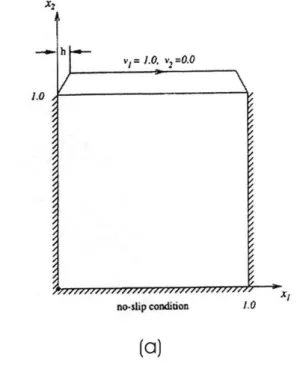
4.4.1 The driven cavity flow problem . . . . 53

4.4.2 The S-channel flow problem . . . . 59

4.5 _{Further study of the FCBI scheme . . . .} 64

4.5.1 Stability of the FCBI scheme . . . . 64

4.5.2 Accuracy of the FCBI scheme . . . . 69

5 A new FCBI 9-node element

5.1 Fluid flow discretization . . . .

79 81

5.2 _{Comparison of the new node element with the earlier published}

9-node elem ent . . . . 92 5.3 _{Comparison of the new 9-node element with the Galerkin 9-node element 97}

6 Linking FCBI to CIP method (CIP-FCBI)

6.1 _{CIP m ethod . . . .}

6.1.1 _{One-dimensional CIP solver . . . .}

6.1.2 _{Two-dimensional CIP solver . . . .}

6.1.3 _{The CIP solver for compressible and incompressible flows} 6.2 Linking the finite element method to the CIP method . . . .

6.2.1 _{The governing equations . . . .}

6.2.2 _{Numerical solutions . . . .} 6.3 Linking the FCBI scheme to the CIP method . . . .

6.3.1 _{The governing equations . . . .}

6.3.2 Numerical solutions . . . .

7 Conclusions

A Consistency of the CIP scheme

B Stability of the CIP scheme

107 . . . 108 . . . 109 . . . 115 . . . 119 . . . 123 . . . 123 . . . 131 . . . 136 . . . 136 . . . 145 151 155 161

List of Figures

2-1 Reference, spatial and mesh configurations . . . . 23

4-1 The two-dimensional incompressible fluid flow problem considered . . 37

4-2 9-node elements and a sub-element in isoparametric coordinates . . . 39

4-3 The demonstration of xi and 1 - x1 functions for the flux through ab for the three different values of q' = 10, q1 = 0 and q1 _{= 200 . . . . . 42}

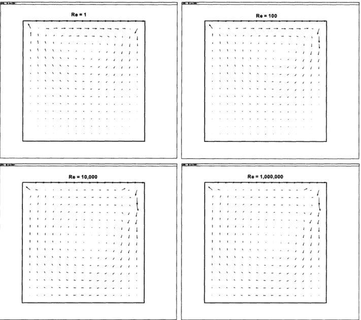
4-4 (a) The driven cavity flow problem (b) The uniform mesh of 8x8 ele-m ents used . . . . 54 4-5 Schematics of solutions for the driven cavity flow problem . . . . 55

4-6 The velocity solutions of the driven cavity flow problem for Re = 1, 100, 10,000, 1,000,000 for the uniform mesh 8 x 8 elements . . . . 56

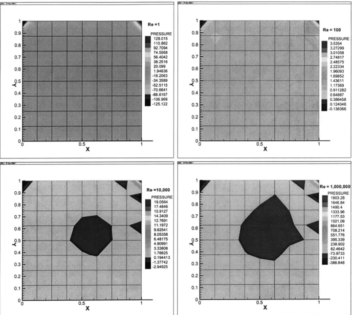
4-7 The pressure solutions of the driven cavity flow problem for Re = 1, 100, 10,000, 1,000,000 for the uniform mesh 8 x 8 elements . . . . 57

4-8 Contours of the vorticity for different Re numbers for uniform mesh 8x 8 elements. The contour levels shown for each plot are -5.0, -4.0,

-3.0, -2.0, -1.0, 0.0, 1.0, 2.0, 3.0, 4.0 and 5.0 . . . . 58

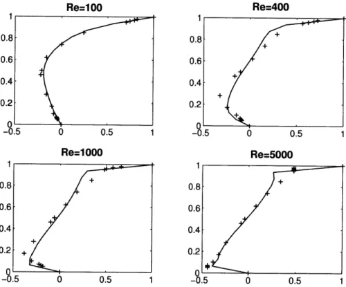
4-9 The horizontal velocity at the vertical centerline of the cavity for Re

= 100, 400, 1000, 5000 when the uniform mesh 8 x 8 elements is used 60

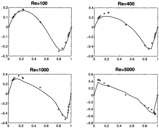
4-10 The vertical velocity at the horizontal centerline of the cavity for Re

= 100, 400, 1000, 5000 when the uniform mesh 8x 8 elements is used 61

4-11 (a) The S-channel flow problem (b) The mesh used . . . . 62

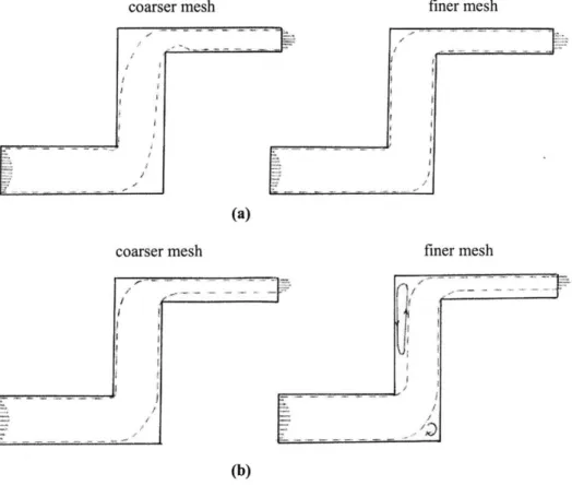
4-12 Schematics of solutions for the S-channel flow problem (a) Re = 100, (b) R e = 10,000 . . . . 63

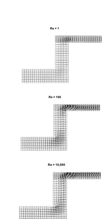
4-13 The velocity solutions of the S-channel flow problem for Re = 1, 100, 10, 000

for the mesh shown in figure 4-11 (b) . . . . 65

4-14 The pressure solutions of the S-channel flow problem for Re = 1, 100, 10, 000

for the mesh shown in figure 4-11 (b) . . . . 66

4-15 Pressure solutions obtained by the FCBI procedure using the mesh shown in Fig. 4-11(b) and the two times finer and coarser meshes when

Re=100 ... ... ₆₇

4-16 Pressure solutions obtained by the ADINA program using the mesh shown in Fig. 4-11(b) and the two times finer mesh when Re = 100 . 68

4-17 The non-uniform mesh of 4x4 9-node elements used . . . . 73

4-18 Comparison of the FCBI 9-node elements, FCBI 4-node elements and the Galerkin 9-node elements for the driven cavity flow problem (Re=1000). In this figure, the x coordinate represents log h when h is the ele-ment size and the y coordinate for each case is a) log IU hf,2 , b)

log

_log

4-19 Comparison of the FCBI 9-node elements, FCBI 4-node elements and the Galerkin 9-node elements for the S-channel flow problem (Re=100). In this figure, the x coordinate represents log h when h is the ele-ment size and the y coordinate for each case is a) log "UJjh1L2 , b)

log IIU"Uh" , c) log IP PhJJL2 , d) log (11 -UhI" I + iP Ph1,i2 )...77

0 I iUII"i IIPiIL2 U1' IIP1iL2

5-1 _{The new FCBI 9-node element (a) The element in its isoparametric}

coordinates, (b) Definition of Axk for the flux through 5-7 . . . . 82 5-2 The demonstration of

f,

# functions for the flux through 5-7 for

the three different values of q1 _{= 10, q}2 _{- 0 and q}3 _{= 200 . . . . 85}

5-3 _{The trial functions h', h' and h' for the flux through 5-7 . . . . 87}

5-4 The earlier proposed 9-node element (consists of four 4-node sub-elements); x1 and (1 - x1) functions are shown for one sub-element and the assemblage of two adjacent sub-elements for high Reynolds number flow when the flux is through 5-7 . . . . 89

5-5 Illustration of Q, and Q.; _{the control volumes of the velocity and}

pressure points respectively . . . . 92 5-6 Comparison of the new FCBI 9-node elements and the original FCBI

9-node elements for the driven cavity flow problem (Re=1000). In this figure, the x coordinate represents log h when h is the mesh size and the y coordinate for each case is a) log IIU-UhjIL2 , b) log " -Uh"H1 , c)

11U11L2 iIUIIH1

log 11PPhj1L2

d)log

9

g IPIL2 , d) lg (IP+ 2 ) . . . . . 96

5-7 Comparison of the new FCBI 9-node elements and the original FCBI

9-node elements for the S-channel flow problem (Re=100). In this figure, the x coordinate represents log h when h is the mesh size and the y coordinate for each case is a) log IIU-Uh L2 _IIUHjL2 , b) log U" _IIUIIH1-Uh1IH1 , c) log IIPPhIL2 d) log (11UUhIIH1 + IP-PhIL2 )...99

iIPIIL2 IIUIIH1 IIPIIL2

5-8 Comparison of the new FCBI 9-node elements and the Galerkin 9-node

elements for the driven cavity flow problem (Re=1000). In this figure, the x coordinate represents log h when h is the mesh size and the

y coordinate for each case is a) log IUUhIL2 _11U11L2 , b) log UUhIH1 , c)

' IUIIH1

log

d)~ log

IIPIIL2 , d o (IU") l IIP1IL2 ) . . . . . 102

5-9 Comparison of the new FCBI 9-node elements and the Galerkin 9-node

elements for the S-channel flow problem (Re= 100). In this figure, the x coordinate represents log h when h is the mesh size and the y coordinate for each case is a) log IUUhjL2 , b) log IUUh H1 , c) log 1'PhjjL2 , d)

1IUIL2 IIU1iH1 IIPIIL2

log (IR7'UhIIH1 + IIP-PhjiL2

)

0

II1H11PIIL210

6-1 The principle of the CIP method. (a) The initial profile and the exact

solution (b) The exact solution at the grid points (c) Linear profile between the grid points (d) The spatial derivative in the CIP method 110

6-2 The 4-node element used in the finite element discretization . . . 127 6-3 The driven cavity flow problem . . . 131

6-4 The non-uniform meshes used for (a) Re = 1000, (b) Re = 10000. . . 133 6-5 Velocity profiles for Re = 1000. . . . . 134

6-6 Velocity profiles for Re = 10000. . . . . 135 6-7 9-node elements and the 4-node sub-element used in the finite element

discretization . . . . 139 6-8 The non-uniform meshes used for (a) Re = 1000, (b) Re = 10000. . . 147

6-9 Velocity profiles for Re = 1000. . . . . 148

Chapter 1

Introduction

The study of incompressible flows is important in many areas of science and tech-nology. At low speeds the flow will be ordered and follow regular patterns, i.e., it is laminar flow. Common applications in which laminar flow appears are biological fluid flow, Newtonian flows in chemical and mechanical engineering and any indus-trial process involving heat, fluid flow and mass transport at low Reynolds numbers.

A balance between the inertia and viscous forces governs laminar flows and provides

the stability. Flows are often characterized by a dimensionless number known as the Reynolds number, which is the ratio of inertia to viscous forces in a flow. Laminar flows correspond to smaller Reynolds numbers. Even though laminar flows are deter-ministic and ordered, instabilities and bifurcation may happen in the flow and take the flow from being laminar to be transition or turbulent. Numerical modelling of transition and turbulence requires greater insight into the flow physics.

For higher Reynolds numbers, the flow is governed by inertial forces and in most cases of engineering problems the flow is in a disordered or turbulent state. Common applications of incompressible turbulent flows involve the flow around vehicles and low speed flows in aeronautics where the fuel efficiency is greatly impacted by the details of the flow.

The Navier-Stokes equations are widely used for the analysis of incompressible laminar flows. If the Reynolds number is increased to certain values, oscillations appear in the finite element solution of the Navier-Stokes equations. In order to

solve for high Reynolds number flows and avoid the oscillations, one technique is to use stabilized methods. In these methods, artificial upwinding is introduced into the equations to stabilize the convective term, ideally without degrading the accuracy of the solution: e.g. the streamline upwind/Petrov-Galerkin (SUPG) method [7], the Galerkin/least-squares (GLS) method [15], the Cubic Interpolated Pseudo/Propagation

(CIP) method [27] and use of the bubble functions [10], [6], [5], [22].

The flow condition-based interpolation scheme (FCBI) is a hybrid of the finite element and the finite volume methods and it was first introduced by KJ. Bathe and

J. Pontaza in [2]. This scheme was later developed in [3], [19] and [20].

The FCBI procedure introduces some upwinding into the laminar Navier-Stokes equations by using the exact solution of the advection-diffusion equation in the trial functions in the advection term. The FCBI procedure is a finite element method since the domain of the problem is considered as an assemblage of discrete finite elements connected at nodal points on the element boundaries, and the velocity and the pres-sure are interpolated within each element. This procedure can also be considered a finite volume method since the weak form of the Navier-Stokes equations is satisfied over control volumes, when the test functions are unit step functions. Hence, the FCBI finite element solution satisfies the mass and momentum conservations for the control volumes (the traditional finite element methods do not satisfy the local mass and momentum conservations).

One reason why the FCBI procedure was proposed as a hybrid of the finite element and the finite volume methods, not being merely a finite volume method, is the lack of defining interpolation functions in the finite volume methods. Defining the interpolation functions enables us to directly evaluate the derivatives, and set up the Jacobian matrix for the Newton-Raphson iteration method. Also, no artificial factors are used and similar to the traditional finite element methods a mathematical theory is available.

The basic aim in developing an FCBI scheme is to reach a numerical scheme that is stable for low and high Reynolds numbers, and yields sufficiently accurate solutions using coarse meshes. Of course, the numerical solution of the laminar Navier-Stokes

equations at high Reynolds numbers would not be highly accurate. The fluid mesh would need to be too fine. However, when a coarse mesh is used, the scheme should still yield a reasonable solution. As the mesh is then refined, the numerical scheme would capture more details in the flow; e.g. circulations, and the solution obtained would ideally converge to the exact solution of the mathematical model. At some stages of the mesh refinement, a turbulent model might be required.

However, in practice, the accuracy of the solution and the computational cost are important issues. These issues are particularly important in the analysis of the fluid flows with structural interactions.

The analysis of fluid flows with structural interactions has captured much attention during the recent years. Such analysis is performed considering the solution of the Navier-Stokes fluid flows fully coupled to the non-linear structural response. However, a fully coupled fluid flow structural interaction analysis can be computationally very expensive. The cost of the solution is, roughly, proportional to the number of nodes or grid points used to discretize the fluid and the structure.

In order for interaction effects to be significant, the structure is usually thin and can be represented as a shell, hence not too many grid points are required. The large number of grid points and consequently number of equations in fluid flow structural interaction problems (FSI) is due to the representation of the fluid domain. For high Reynolds number fluid flows, to have a stable solution, more grid points are required. In order to decrease the number of grid points in the fluids (using a coarser mesh) and still have a stable solution, the flow-condition-based interpolation (FCBI) procedure was introduced [2], [3], [4].

The basic philosophy of FCBI scheme was presented earlier in [2]. However, our aim is to increase the effectiveness of this scheme. The previous works on the FCBI procedure include the development of a 4-node element and a 9-node element consisting of four 4-node sub-elements. In this thesis, the stability, the accuracy and the rate of convergence of the already published FCBI schemes is studied in section 4.5, and it is shown that the FCBI 4-node elements and the earlier proposed FCBI 9-node elements obtain more stable solutions than the Galerkin 9-9-node elements, used

in the traditional finite element methods. However, the Galerkin 9-node elements give more accurate solutions with a higher rate of convergence. Our objective is to use the FCBI scheme in rather coarse meshes together with the "goal-oriented error measurements" technique to control error in the structural response in the fluid flow structural interaction problems [12]. Hence, in chapter 5 we propose a new FCBI 9-node element that obtains more accurate solutions than the earlier proposed FCBI elements. The new 9-node element does not obtain the solution as accurate as the Galerkin 9-node elements but the solution is stable for much higher Reynolds numbers (than the Galerkin 9-node elements), and accurate enough to be used to find the structural responses.

In chapter 6, the focus is on the Cubic-Interpolated Pseudo-particle (CIP) method. The CIP method was introduced by T.Yabe et al. in 1991 [26], [17] . In this method, a cubic polynomial is used to interpolate spatial profiles and spatial derivatives. The spatial derivative itself is a free parameter and satisfies the master equation for the derivative. After the values have been found, the same values for the next time step are simply calculated by shifting the cubic polynomial.

The CIP scheme is a very stable finite difference technique that can solve gener-alized hyperbolic equations with 3rd order accuracy in space. In this thesis, in order to solve the Navier-Stokes equations, the CIP scheme is linked to the finite element method (CIP-FEM) and the FCBI scheme (CIP-FCBI).

The thesis is organized as follows. In Chapter 2 a brief review of the contin-uum governing equations for fluid flows is given, which includes the definition of the Eulerian formulation, the conservation equations and the equations of motion. Chapter 3 describes the finite element discretization of those governing equations. Chapter 4 is devoted to the introduction of the FCBI procedure, the discretization of the FCBI scheme for the earlier proposed 9-node elements (consisting of four 4-node sub-elements), the solution of some numerical examples and a further study of the FCBI scheme for these elements. Subsequently, in Chapter 5, a new FCBI 9-node element is proposed and compared with the former FCBI 9-node element and the Galerkin 9-node element. In Chapter 6, a review of the CIP method is given.

Then, in order to solve the Navier-Stokes equations, the CIP scheme is linked to the finite element method (CIP-FEM) and the FCBI scheme (CIP-FCBI) respectively. Finally, in Chapter 7 the conclusions of this work are given and future research in the development of the FCBI scheme is suggested.

Chapter 2

Governing equations of continua

In physics, materials are divided into three classes; solids, liquids and gases. In fluid mechanics, there are only two classes of matter: fluids and non-fluids (solids). In solid mechanics, one might follow the particle displacements since particles are bonded together. However in fluid mechanics, one's concern is normally the fluid velocity.

Consider the rigid-body dynamics problem of a rocket trajectory. We are finished after solving for the paths of any three non-collinear particles on the rocket since all other particle paths can be reached from these three paths. This scheme of following the trajectories of individual particles is called the Lagrangian description of motion and is very useful in solid mechanics.

But consider the fluid flow out of the nozzle of that rocket. Of course we cannot follow the millions of separate paths. Even the point of view is important, since an observer on the ground would see a complicated unsteady flow, while an observer fixed to the rocket might see a nearly steady flow of regular pattern. Thus it is useful in fluid mechanics to choose the most convenient origin of coordinates to make the flow appear steady, if it is possible, and to study the fluid velocity as a function of position and time, not to follow any specific particle path. This scheme of describing the flow at every fixed point as a function of time is called the Eulerian formulation of motion. In this chapter first the Eulerian formulation is briefly discussed, then the governing equations of Newtonian flows are considered.

2.1

Eulerian formulation

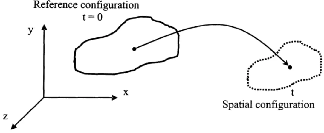
Consider a body that is moving from a reference configuration, the space occupied by the body at time t = 0, to the spatial configuration, the space occupied by the body

at time t (see figure 2-1).

In the Lagrangian formulation, each fluid particle is labelled by its reference po-sition ro at time t = 0, giving velocity functions such as v = v(ro, t). In the Eulerian formulation, a velocity field is specified by

v = v(r, t) = v(x, y, z, t) (2.1)

That is, the velocity for time t is defined at the fixed spatial position r. By defining this velocity, we can obtain a complete kinematic description of the flow. However, this function is not in general known in advance. The fixed spatial position r can be related to the reference position ro as

r = p(ro, t) (2.2)

If

Q represents any property of the fluid, in the Eulerian formulation

Q

by

Q

If dx, dy, dz and dt represent arbitrary changes in the four independent variables (x, y, z, t), the total differential change in

Q

OQ

Q

OQ

dQ= - dx+ dy + dz+ dt (2.4)

Ox ay z at

For velocity components (vi, vY, vz), the spatial increments must be such that

dx = vx dt dy = vy dt dy = vz dt (2.5)

Reference configuration t = 0 y _ _ _ _ _ t Spatial configuration z

Figure 2-1: Reference, spatial and mesh configurations

DQ

Q

Q

(2)Q

- +v -

+vy

Dt

at

The quantity 9 _Dt is called material derivative or particle derivative which shows that we are following a fixed particle. In this equation, 9 is the local derivative and the last three terms are called convective derivatives. The vector form of this equation is written as

DQ _

Q

Dt - + (v - V)Q

(2.7)

2.2

Conservation equations

Consider a material volume moving from position ro at time t = 0 to the new position

r at t (see figure 2-1). The material volume is an arbitrary collection of matter enclosed by a material surface (or boundary) and every point of which moves with the local fluid velocity. This surface is hypothetical and in general does not correspond to any physical boundary in the flow. As the material volume moves through space, it is deformed in shape and changed in volume. We will refer to the material volume as Q(t). The dynamical laws of motion are stated for the material volume and are as follows: Conservation of mass (continuity), Balance of linear momentum (Newton's

second law), Balance of energy (first law of thermodynamics) and Creation of entropy (second law of thermodynamics).

The first law, continuity, means that for a material volume the mass is constant. Newton's second law, momentum conservation, states that the rate of change of the volume momentum (momentum per unit volume) is equal to the sum of the surface forces (due to pressure and viscous stresses) and body forces (such as gravity) acting on it. From the first law of thermodynamics, the rate of change of the material-volume energy (internal plus kinetic) is equal to the rate at which forces do work upon it plus the rate at which heat is transferred to it. Finally, the second law of thermodynamics states that the change of internal entropy is greater or equal to the external entropy

supply (due to the heat supply).

Our focus in this work is on isothermal processes of incompressible fluids. Hence, we only consider the mass and momentum conservations in this chapter.

2.2.1

Mass conservation

For a material volume the mass is constant, so that the conservation of mass takes the form

Dm f _{p(r)dQ = 0}

(2.8)

Dt _{Dt (t)}

where Q(t) is the material volume, m is the total mass enclosed in Q(t) and p is the material density.

The differential equation of mass conservation can be derived from the integral equation with the application of the divergence theorem, and making use of the fact that the material volume is arbitrary. In the Lagrangian formulation, this equation is written as,

p(ro) = det (t X) _(2.9)

p(r)

where ('X) is the deformation gradient (see [1]). In the Eulerian formulation, this is equivalent to

Dp +pVV -V= 0 _(2.10)

Dt

where v is the material velocity. If the density is constant (incompressible flow), this equation reduces to

V - v = 0 (2.11)

2.2.2

Momentum conservation

This law is called Newton's law of motion and it states that the rate of change of the material volume momentum is equal to the sum of all external forces acting on the body at time t.

DP _Fext

(2.12)

Dt Zex

where P is the momentum of the material volume. This equation can also be written as

D f pvdQ = Fext(t) _(2.13) The differential equation of the above equation in Eulerian formulation is

D(pv) y = fbi + fb2 _(2.14)

Dt

where fbood is the applied force on the fluid particles per unit volume, and contains

two types of body forces: fbi, the gravitational body force (we only consider the gravitational force here) and fb2, which is the body force that satisfies the equilibrium. In the Lagrangian formulation, Newton's second law is easily written as Fext = m a,

where m is the mass and a is the acceleration of the body.

As it was already mentioned, only the gravitational body force is considered here and fbi = p g, where g is the acceleration of gravity. The fb2 force satisfies equilibrium for the external stresses applied on the body and can be expressed as f42 = V -T,

where T is the stress tensor. The momentum conservation then becomes

D(pv) _{P g + V -T}

(2.15) Dt

2.3

Equations of motion

The Navier-Stokes equations are derived from the momentum and mass conservation equations (2.15) and (2.10). It remains only to express T in (2.15) in terms of the

velocity v. This is done by relating Tij to eij , the (ij) th components of the stress and velocity strain tensors, through the Newtonian fluid constitutive law,

Tij = -p 6ij + 2/teij (2.16)

with

1

ei= = (vij + Vji) (2.17)

where p is the pressure and p is the dynamic viscosity coefficient. The non-conservative form of the Navier-Stokes equations is obtained by substituting the stress relations

(2.16) into Newton's law (2.15) as

Dv

p_ =pg-Vp±+pV2_{v (2.18)}

Dt

The boundary conditions required to solve the Navier-Stokes equations can be given as follows:

v = vs on S, (2.19)

Tn = t on Sf (2.20)

v(to) = vo (2.21)

where S, is the part of the fluid boundary with imposed velocities v, Sf is the part of the boundary with imposed surface tractions t and n is the unit outward vector normal to the fluid boundary.

The momentum equation (2.15) can also be written as

ovi

pv + F, j = pgi (2.22)

where

Fij, j = pvjvi -Tij (2.23)

The above form is referred to as the conservative form of the momentum equation since for any material volume Q(t) of the fluid, using the divergence theorem

f _n(t) Fi, j dQ = _'sMtFiSnt dS (2.24)

where S(t) and the nj are the material surface and the components of the unit vector normal to S(t) respectively. Note that in the FCBI scheme, the conservative form of the momentum equation is used.

The Navier-Stokes equations are widely used for the analysis of incompressible viscous flows. However, viscosity is assumed to be constant in these equations and for non-isothermal flows, particularly for liquids whose viscosity is highly temperature-dependent, the Navier-Stokes equations may not be a good approximation. In our work, we only consider isothermal processes of incompressible fluids and the Navier-Stokes equations are used.

Chapter 3

Finite element formulation

In this chapter we consider the finite element formulation and solution of the Navier-Stokes equation given in (2.11) and (2.16).

Using index notation for a stationary Cartesian coordinate system (xi, i=1,2,3), the Navier-Stokes equations (2.11) and (2.16) of incompressible fluid flow with in the domain Q are (at time t),

pOv p

(a

and eij represents components of the velocity tensor and is given as,

1

eij = (vi, j + vj, 2) (3.3)

Using index notation, the boundary conditions (2.19) and (2.20) are written as,

Ti nh1= f on Sf (3.5)

where S, is the part of the fluid boundary with imposed velocities 0f, Sf is the part of the boundary with imposed surface tractions

fA

The finite element solution of the Navier-Stokes equations (3.1) is obtained by considering a weak form of these equations. Using the Galerkin procedure (the test functions correspond to the finite element interpolations), the weak formulation of the problem can be given as:

Find v E H'(Q) with v = vs on So, and p E H1(Q) such that

j V P i ±vi, vi dQ + Eij Tii dQ= jifiBd jVf+ V S 3.6S n P vi, i dQ = 0

for all V E H1(Q) with V = 0 on Sv and p E H1(Q).

In the above expressions the overbar sign denotes the virtual quantity, the Sobolev space Hk (Q) (for any non-negative integer k) is defined as the space of square inte-grable functions over Q, whose derivatives up to order k are also square inteinte-grable over Q.

In equations (3.6), the mixed-formulation is used (the velocity and the pressure are both considered as variables), and the momentum equation is weighted with the virtual velocity while the continuity equation is weighted with the virtual pressure. These equations must be discretized in space in order to be solved numerically. The following finite element spaces are introduced for the velocity and pressure,

Vh = vh E H1(Q)

V =VhH(Q)(3.7)

Qh -ph E H1 (Q)

h - jh _{E H (Q)}

Then, the finite element problem can be stated as:

Find vh E Vh(Q) and ph E Qh(Q) such that

j Vp + j dQ + f ;Tih dQ= j fB dQ + (Vh)S fis dS

J

(3.8)

for all Vh E Vh (Q) with Vh = 0 on S, and p E Qh (Q)

In the finite element procedure, the space Vh depends on the elements chosen to discretize the volume Q. In a 2D space, we can choose, for example, quadrilateral bilinear or parabolic elements. The pressure interpolation, however, cannot be chosen arbitrary (see for example [1]), otherwise, the formulation may not be stable. In order to have stability, the inf-sup condition must be satisfied. A list of the effective v/

p (velocities are continuous between elements) and v/ p-c elements (velocities and

pressures are both continuous between elements) are given in table (4.6) and (4.7) in [11.

Using any of these elements (that satisfy the inf -sup condition) to discretize equa-tions (3.8) in steady-state two-dimensional planar flow analysis, the governing matrix equations for a single element are then,

K_{VXP Av}

KVYP _AVy

0 AP

R< F<)

0 Fp

In these equations, Av, Av., Ap, are the increments of the velocity in the x

direction, the velocity in the y direction and the pressure with respect to the last iteration; Rvx and R,, are the discretized load vectors and FvX, F,,, FP contain terms from the linearization process [1].

If H' and HP contain the interpolation functions for the velocities and the

pres-sure respectively, the elements of the stiffness matrix are

Kvxvx KV,,X KPy, KVY 1K V₁ VY KPVY (3.9)

Ky2,= [2p (H"f)T Hvx + p (H"Y)T Hv ] dQ + [(Hv)T Hvvx Hvx + (Hv)T Hvvy Hv] dQ K,,,,=

f

Since in this work, we only consider the incompressible fluid flow, KP 0 and Ap cannot be statically condensed out for each element.

For a fluid flow problem, the solution obtained using the discretized equations

(3.9) and (3.10) is good for low Reynolds number flows ( laminar flows). However, if

due to the presence of the convective terms vi, j vj in equations (3.6).

Before we discuss how to avoid these oscillations, we mention that, of course, after Reynolds number is increased to a certain range, the flow condition turns from laminar to turbulent, and a turbulence model should be used. However, the turbulent flow could still be solved using the laminar Navier-Stokes equations. In order to increase the accuracy of the solution for high Reynolds number flows, the mesh need to be too fine and the analysis can be computationally very expensive.

In order to solve the high Reynolds number flows, one technique is to use stabilized methods. In these methods, artificial upwinding is introduced into the equations to stabilize the convective term, ideally without degrading the accuracy of the solution. Different stabilized methods have been proposed and compared in various papers, i.e. the streamline upwind/Petrov-Galerkin (SUPG) method [7], the Galerkin/least-squares (GLS) method [15] and use of the bubble functions [10], [6], [5], [22].

Among all the proposed stabilized methods, this thesis focuses on two of these methods; the flow-condition-based interpolation (FCBI) procedure [2] and the Cubic Interpolated Pseudo/Propagation (CIP) method [27]. The FCBI procedure intro-duces some upwinding into the laminar Navier-Stokes equations by using the exact solution of the advection-diffusion equation in the trial functions in the advection term. Chapter 4 is devoted to the introduction of the FCBI procedure, the dis-cretization of the FCBI scheme for the earlier published 9-node elements (consist of four 4-node sub-elements), the solution of some numerical examples and the stabil-ity and convergence study of the FCBI scheme for these elements. Subsequently, in Chapter 5, a new 9-node FCBI element is proposed and compared with the former FCBI 9-node element. In Chapter 6, the focus is on the CIP scheme. This chapter begins by reviewing the CIP procedure, then linking the CIP scheme to the finite element method (CIP-FEM) and finally to the FCBI procedure (CIP-FCBI).

Chapter 4

Flow-condition-based interpolation

scheme (FCBI)

The flow condition-based interpolation scheme (FCBI) is a hybrid of the finite element and the finite volume methods and it was first introduced by KJ. Bathe and J. Pontaza in [2]. This scheme was later developed in [3], [19] and [20].

As it was mentioned earlier in chapter 3, if the Reynolds number is increased to certain values, oscillations appear in the traditional finite element solution of the lam-inar Navier-Stokes equations. In order to solve the high Reynolds number flows and avoid the oscillations, one technique is to use stabilized methods. In these methods, artificial upwinding is introduced into the equations to stabilize the convective term, ideally without degrading the accuracy of the solution.

The FCBI procedure introduces some upwinding into the laminar Navier-Stokes equations by using the exact solution of the advection-diffusion equation in the trial functions in the advection term. The FCBI procedure is a finite element method since the domain of the problem is considered as an assemblage of discrete finite elements connected at nodal points on the element boundaries, and the velocity and the pressure are interpolated within each element. This procedure is also considered as a finite volume method since the weak form of the Navier-Stokes equations is satisfied over the control volumes, when the test functions are unit step functions. Hence, the FCBI finite element solution satisfies the mass and momentum conservations for the

control volumes (the traditional finite element methods do not satisfy the mass and momentum conservations).

The main reason the FCBI procedure was proposed as a hybrid of the finite element and the finite volume methods, not merely a finite volume method, is that interpolation functions are not defined in the finite volume methods. Defining the interpolation functions enables us to directly evaluate the derivatives, and set up the Jacobian matrix for the Newton-Raphson iteration method.

In this chapter first the review of the FCBI procedure is given for the earlier published 9-node element (consists of four 4-node sub-elements) [3]. Then, the effec-tiveness of this method is tested by solving some numerical problems. At the end of this chapter, the stability and convergence study of this method is presented.

4.1

The governing equations

We consider the conservative form of the Navier-Stokes equations of a two-dimensional incompressible fluid flow within the domain Q at time t (figure 4-1),

a + V - (pyv - -r) = 0 (x, t) E Q X [0, T]

at _(4.1)

V - (pv) = 0 (x, t) E Q x [0, T]

subject to the (sufficiently smooth) initial and boundary conditions

v(x, 0) = vO (x)EQ p(x,O) = po (x) E Q (4.2) v =v (x, t) E Sv x (0, T) we -n = fr (x t) E Sf x (0, T) where

7 = ' (v, p) = -p I + p [Vv + (Vv)T] (4.3)

In equations (4.1-4.3), p is the viscosity, p is the density, vs are the prescribed velocities on the boundary S, f5 are the prescribed tractions on the boundary S1

(S = S, U Sf, S,

n

Sf

SV

Figure 4-1: The two-dimensional incompressible fluid flow problem considered

The finite element solution of the Navier-Stokes equations (4.1) is obtained by considering a weak form of these equations. Using the Petrov-Galerkin procedure (the test functions do not correspond to the trial functions), the weak formulation of the problem can be given as

Find Vh E Vh, Uh E Uh and Ph E Ph such that

Io

where Wh E Wh and qh E

Qh-Note that in these equations, the convective term (pvv) in equation (4.1) is

re-placed by (puhvh) in the weak formulation where Vh C Vh and Uh E Uh (two different

defined for the same nodal velocity variables). The idea of using these two different spaces lies in that it is the convective term that for high Reynolds numbers introduces the instability and oscillation in the numerical solution . Hence, the convective term needs to be interpolated exponentially. Therefore, we replace the convective term

(p VhVh) by (p UhVh) and we define the interpolation functions to be exponential in

Vh and linear in Uh. Another reason is that then the FCBI scheme is also applicable to any other transport equation, for example, the advection-diffusion equation where, in the convective term, the temperature would be interpolated in V and the velocity in Uh.

4.2

The fluid flow discretization

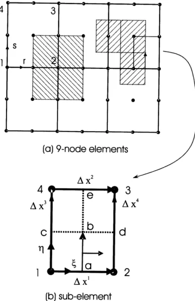
The spaces used in the finite element procedure depend on the elements chosen to discretize the volume Q. In this chapter, we consider the earlier published 9-node element (consists of four 4-node sub-elements) [3].

A mesh of elements is shown in its natural coordinate systems in figure 4-2. Each

9-node element is defined in the r - s coordinates with 0 < r, s < 1.0 and consists of

four 4-node sub-elements. Each sub-element is defined by four nodes of the 9-node element and is used for the interpolation of velocities. The pressure is interpolated by the four corner points in each element. Hence, for the definition of the spaces V, Uh

and Ph, we refer to the sub-elements and elements respectively. The sub-element is

defined in - q coordinates with 0 < , q K 1.0. To obtain the matrices or derivatives

in x - y coordinates, the usual isoparametric transformation is used [1].

The trial functions in Uh _{are defined in each sub-element as,}

hu hu 1

-or4 = - (4.5)

hu hu"

4 s 3 S\\ X. %04 I

₂

4

Figure 4-2: 9-node elements and a sub-element in isoparametric coordinates

K

/*

I

4V .... ... ,]

I

(a) 9-node elements

A X2

a

e

Sa

3

d

(4.6)

with 0 , r <1.

Similarly, the trial functions in the space Ph are given in each element as,

[

I

The trial functions in V are defined using the flow conditions along each side of the sub-element. The functions are, for the flux through ab (Fig. 4-2),

1-x 1 1-x21 I 2

[

[

)

[

-

h v = (1 -x 1) (1 - 77)2 + (1 -- X2) (1--r) h2 =x(1 - rn)2 + X2(1 _ n h V = X1 (1 - r1)r7 + X2772 hv = (1 - x1)(1 -77)7 + (I -x 2₎₇2 e ____ k pi. fl AXk xk , = _,q = X eqI _q with (4.10) (4.11)

where ti E Uh and is the velocity at the center of the sides considered

(

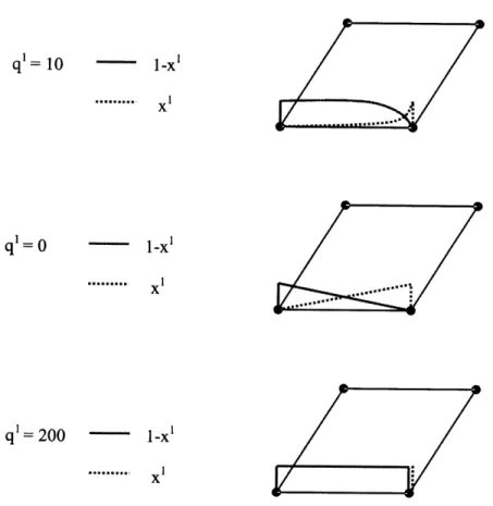
To demonstrate these functions in more details, functions x' and 1 - xi are shown

in Fig 4-3 for three different values of q1 = 10, qI = 0 and q1 = 200.

As we see in figure 4-3 for the case q' = 0 , when qk goes to zero, the xk function approaches , and hv functions approach the linear functions hj .

Note that M functions for the flux through ab in Fig 4-2 for example, are

exponen-tial functions in the direction of the flow and linear in the other direction (functions

xk and 1 - xk are interpolated linearly for the other direction). hv is, for example,

1-x1 for

(1- ) for

0 < < 1.0, 77 = 0 0 77 1.0,( = 0

Analogously, the hj functions are defined for the flux through bc as,

l= 10 - 1-xI qg=O

1-x

Figure 4-3: The demonstration of x1 _{and 1 - x}1 _{functions for the flux through ab for} the three different values of q' = 10, q1_{= 0 and q}1_{= 200}

(4.13) h

v

where fii E Uh and is the velocity at the center of the sides considered ( r7 = 1 and = _{0, 1 for k} = 3, 4 respectively).

Note that the trial functions hj satisfy the requirement E h = 1.

The elements in the space Qh are step functions. have, at node 2, for example,

Referring to Fig. 4-2(a), we

1 for (r,s) E[ [ ,1] x [0, 1] 0 elsewhere

(4.15)

Similarly, the weight functions in the space Wh are also step functions. Considering the sub-element shown in Fig. 4-2(b), at node 1, for example,

1 for (, r) E [0, ] x[0, ] (4.16)

0 elsewhere

Then, the velocities Uh, Vh (in each sub-element) and the pressure Ph (in each

4 Uh = ( h Vhi i=1 4 Vh = ( hv Vh (4.17) i=1 4 Ph = h' Phi i=1

where Vhi and Phi are the nodal velocity and pressure variables.

We again mention that although two different spaces are defined for the velocities but of course h and hy functions are defined for the same nodal velocity variables Vhi.

The idea of using these two different spaces lies in that it is the convective term that for high Reynolds numbers introduces the instability and oscillation in the numerical solution. Hence, the convective term needs to be interpolated exponentially. We

replace the convective term (p VhVh) by (p UhVh) and we define the interpolation

functions to be exponential in V and linear in Uh. Another reason is that then the FCBI scheme is also applicable to any other transport equation, for example, the advection-diffusion equation where, in the convective term, the temperature would be interpolated in V and the velocity in Uh.

Considering the steady-state condition, equation (4.4) is then,

jWhV [P UhVh - Th(UhPh)] dQ = 0 (4.18)

j qhV (p Uh) dQ = 0

Assembling equations 4.18 for all the control volumes in the body, and using the divergence theorem to take these integrals around the control volumes we get

S

qS h n- (p Uh) dS = 0

where the momentum and the continuity equations are summed over the control volumes of the velocity points and pressure points respectively, S is the surface of each control volume (that corresponds to the length in two-dimensional problems), n is the unit normal vector pointing to the outside of the control volume and

Th -Ph I + Y [VUh + (Vuh)T] (4.20)

The flux is then calculated with the interpolated values at the center of the sides of the control volumes. For example, the flux through ab (Fig. 4-2) is obtained as

f n -f dS = n - 1'()=1/, 71=1/4 ASab (4.21)

where ASab is the length of ab and

f(6) = p UhVh + Ph I - A [Vuh + (Vuh)T] (4.22)

in the momentum equation and

f(6) = p Uh (4.23)

in the continuity equation.

Replacing Uh, Vh and Ph from the equations (4.17) , when wh and qh are the unit

step functions (for the control volumes of the velocity and pressure points respec-tively), the corresponding linearized finite element matrix equations are,

C

Ii Ii

where Av2, Avy, Ap, are the increments of the velocity in x direction, velocity in

y direction and pressure with respect to the last iteration; Rvx and Ry are the

dis-cretized load vectors and Fv,, Fvy, FP contain terms from the linearization process. Using the full Newton-Raphson iteration method, for a mesh of non-distorted ele-ments, we get K~~ (j,i) = _{Whj A} Wh /i nx Oy 0

Whi/i x y a

Thja

axn

a

Ox Or

O(gmhv

+ _{Whi /i ny}

Ox

[ O(M h) (Vhm)xj

K,,,(j,i) = Whj nx

+