Active Focus and Zoom Control Used for Scene Analysis

HAL Id: hal-00554164

https://hal.archives-ouvertes.fr/hal-00554164

Submitted on 11 Jan 2011

HAL is a multi-disciplinary open access archive for the deposit and dissemination of sci-entific research documents, whether they are pub-lished or not. The documents may come from teaching and research institutions in France or abroad, or from public or private research centers.

L’archive ouverte pluridisciplinaire HAL, est destinée au dépôt et à la diffusion de documents scientifiques de niveau recherche, publiés ou non, émanant des établissements d’enseignement et de recherche français ou étrangers, des laboratoires publics ou privés.

Active Focus and Zoom Control Used for Scene Analysis

David Bailly, Philippe Gaussier

To cite this version:

David Bailly, Philippe Gaussier. Active Focus and Zoom Control Used for Scene Analysis. Proceedings of the 2010 International Conference of Soft Computing and Pattern Recognition, Dec 2010, Cergy-Pontoise, France. pp.P192. �hal-00554164�

Active Focus and Zoom Control Used for Scene

Analysis

David Bailly, Philippe Gaussier

Neurocybernetic team, ETIS, CNRS UMR 2051, ENSEA, University Cergy Pontoise, F-95000 Cergy Pontoise www-etis.ensea.fr

[email protected], [email protected]

Abstract—We propose a visual recognition system for robotic applications in which distance to the visual objects can change a lot (for instance, trying to recognize a distant object learned from a short distance). Our system takes advantage of a single pan-tilt camera controllable in zoom and focus. Focus control allows to detect plans of sharpness in the scene and indirectly to compute a distance. Hence, this information can be used to gain structural information of the visual scene (to segment objects from the ground, to count the number of depth plans in the visual field...) without complex computation. This distance information is then used to control either a software or a hardware zoom to keep the size of the object invariant. The image thus created can be used by view based recognition systems. In a second time we show how by using focus points and neural networks we can improve the detection of sharpness plans in complex scenes. Finally we present a simple method to dynamically control the focus and stabilize it on the plan of sharpness of an object in the scene.

Index Terms—vision; depth perception; scene analysis; focus control;

I. INTRODUCTION

New humanoid robots and other autonomous navigation systems face the problem of recognizing different kinds of objects from a wide variety of distances. For instance, a new object can be presented from a short distance to the robot (typically 1 m) and next the robot can be asked to find this object from a longer distance (ie 5 to 8 meters). To insure a consistency in the size of objects several solutions have been proposed. The first one considers the use of 2 coupled low resolution cameras: one with a large field providing a peripheral vision and a second one with a narrow field of view providing an image similar to the fovea. These systems require an active pan-tilt control to direct the robot gaze on the object to recognize [1]. The second solution is to use a software fovea on a high resolution camera. Transferring only the ”foveal” part of the image allows to come back to real time computation. To gain distance information necessary for object manipulation, 3D recognition can be performed from 2 distant static cameras or can be actively obtained from the focus of the two camera on the same point in the image. Yet, depending on the distance between both cameras, the precision can be rather limited for distant objects and/or the computational cost and its complexity increases a lot [2].

To solve those problems we chose to take advantage from a single camera with controllable focus and zoom. The focus control provides sufficient information on distance to keep the size of an object constant in the vision field. The object

distance is computed using defocus techniques by sweeping the whole range of values and selecting the the value for which the standard deviation on the pixel of the image is maximum. Several similar techniques have been proposed starting with [3] and more recently [4] and [5]. With the distance and by using the physical or a software zoom the system is able to stabilized the size of an object to a reference size (for example the size linked to the distance used during a training phase). This corrected image can then be used by a recognition system thus avoiding all the rescaling problems.

Finally we present a system based on neural networks able to isolate the different plans of sharpness in a scene and control the focus to stabilize the vision on one of those plans.

II. FROMSTANDARDDEVIATION TOCONSTANTSIZE IN THEVISIONFIELD

In robotic navigation several approaches are used to get depth information. For example, visual looming uses the relative size of objects in the field of view to detect there relative distance to the robot [6]. The variation in the size becomes more important as the robot comes closer to the object.

Another technique using the dynamic of the system is pre-sented in [7]. It uses a grid of pixels chosen in the visual input at regular intervals to compute the distance on the color vector for those pixels. Brutal changes from one time frame to the next indicate the apparition of an object in the field of view. A map of the environment is then created with those points giving the base for navigation.

Our system (Fig. 1) is based on the dynamic of the camera and more precisely on the focus. The idea of the first experiment was to insure a constant size of an object in the visual field. The system uses a reference plan (for example the plan used during a learning phase for a learning system) and compare that value to the current focus value to compute the needed correction in the zoom.

We used a MTV-54g10h camera, PAL 640x480 pixels, with focus and zoom controllable by serial port. Through serial bus we transmit and receive focus and zoom information. It is also equipped with a classical video output linked to our computer. The camera is set on a pan-tilt system allowing a large exploration of the visual environment. (We will not here described the part of the researches on the tracking and centering of the object). We will assume that

Fig. 1: Overview of the first experimental setup. The video input goes through the vision bloc where computation of standard deviation are made. This information is then used by the control bloc to stabilize the focus value on the plan of sharpness. When stabilize the needed correction in the zoom are computed and applied in the zoom bloc.

all needed movements to center the camera on a specific area of the environment has been completed prior to the computations. The computations are performed by neuron emulation program called Promethe running on a simple computer. The control architecture is split into the three following parts (see fig. 1).

The basic image computations are done in parallel to the rest of the system in the vision network. This includes transforming the image from RGB color to gray levels and computing the global standard deviation. After transformation the image is a matrix of float values between 0.0 and 1.0. To compute the standard deviation we used 32x24 pixels area in the center of the field of view. In that area 500 pixels are chosen randomly at the beginning of the experiment. They form a vector on which the standard deviation is computed (equations (1), (2), (3)). This gives a fairly good appreciation of the sharpness of the image. Those pieces of data are then transmitted to the control part.

µ(M ) = 1 I ∗ J I X i=1 J X j=1 Mi,j (1) V ar(M ) = 1 I ∗ J I X i=1 J X j=1 (Mi,j− µ(M ))2 (2) σ(M ) =pV ar(M ) (3)

where M the local matrix ofIxJ pixels,µ(M )is the mean

value of the matrix M, V ar(M ) the variance andσ(M ) is

the standard deviation.

The control network uses the standard deviation to find the sharp focus plan. This is done by sweeping the whole range of focus and finding the maximum. That value is then used to stabilize the image at the sharp focus (Fig. 2). The information on standard deviation value is also used to refocus when needed. A brutal variation in the standard deviation is assumed to be related to an important change in the image and will trigger a new focus sweep.

Fig. 2:Standard deviation during a focus sweep. The scene had only one sharp plan at 1 meter. We clearly see the maximum at the expected distance.

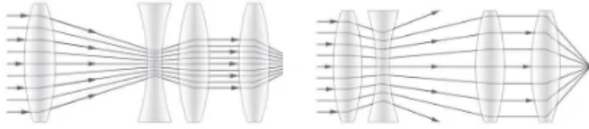
Fig. 3:Coarse description of the lens system in a zoom and focus adjustable camera. The mobile lenses are in between the fixed ones. A movement of one of the lenses will inevitably affect the range of movement of the other.

After stabilization of the image, the zoom and the focus data can be used for the following blocs. For our researches we didn’t use the physical zoom. The reason is that a variation in the value of the physical zoom create a variation on the range of focus values. For a minimum zoom (x1) the camera offers 17 focus positions when for a maximal zoom (x10) we get 465 positions. This is due to the construction of the camera (Fig. 3). When one of the lens is moved the physical range of movement of the other is modified. In our system the zoom is the master lens. This problem can be solved by building a correspondence table to associate the focus plan with the value for each zoom position. But even then the problem of low resolution in the range of focus values will subsist. We solved this problem by using a software computed zoom done in the zoom network. It is made possible by the use of an image of smaller size (320x240) in the system than the one captured by the camera (640x480). Thus we limit the loss in resolution. A linear smoothing is applied to the output image in order to avoid artifacts for the following parts of the system (Fig. 4). Finally the image can be used by other parts symbolized by the learning bloc in our case.

The experiment shows that the precision of the focus value is linked to the zoom value beside the problem already addressed previously. For example, if the physical zoom is x6, 75% of

Fig. 5:Global standard deviation computed on the scene with the 3 boxes. 5000 points where chosen randomly in the whole image and used to compute the standard deviation. We can clearly see the 3 peaks at 40, 70 and 100cm corresponding to the 3 objects in the scene.

the dynamic is in the first meter from the camera. Only 25% are left to detect distances between 1 meter and infinity. We set the physical zoom to its maximum value for most of the tests. The standard deviation is also sensitive to the texture of the object. For a smooth object the noise is a problem. This can be partly solved by a temporal smoothing of the captured images. It is a compromise between speed and robustness.

III. SCENEDEPTHMAP ANDZOOMCONTROL

Moving forward with the same idea we explored more possibilities offered by the controllable focus. The system still uses a focus sweeping method.

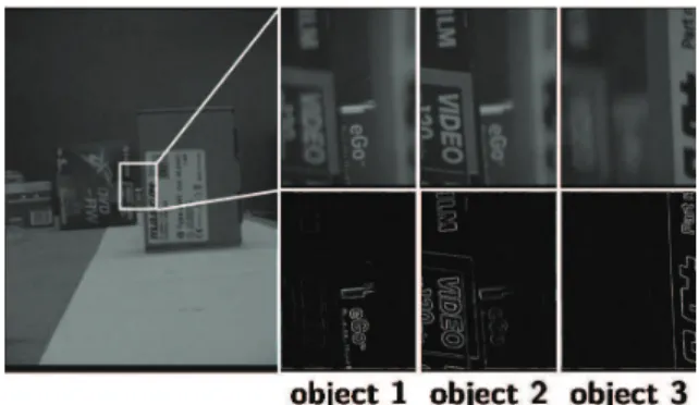
First we used the same technique as in [4] using a 3x3 local mask to calculate a standard deviation for each pixel. As shown in Fig. 6 the 3 different objects present in the scene can be identified by the depth perception. Due to the non linearity of the equations ruling optic systems it is harder to differentiate object 1 from object 2 than object 2 from object 3 even if they are at the same distance from each other. This comes from the term in 1

u in equation (4) (see also Fig. 7).

For u1 andu2 such asu1 < u2 and the same variation ∆u

then 1 u₁+∆u> 1 u₂+∆u. 1 u+ 1 v= 1 F (4)

with u the lens to object distance, v the lens to sensor distance and F the focal length.

In a second time, we used a system based on points of interest. Our navigation and object or facial recognition systems already use points of interest to extract information from a scene as follows. A gradient of the input image is computed and then by convoluted with a difference of gaussians. The local maxima selected in the output of those filters are the points of strong curvature. The system then computes a local standard deviation on a local view selected around those points. By taking several points of interest it is possible to increase the robustness of the computation. As shown in figure 8 we still find the 3 objects present in the scene. Compared to the simple computation (Fig. 5)we can

Fig. 6: Example of depth map using a local 3x3 mask to compute the standard deviation of each pixel. Three objects were present in the field of view at respectively at 0.4, 0.7 and 1 meter. Top images are the view provided by the camera and bottom images are the respective computed maps.

Fig. 7:Relation between distance and focus value. The line is the average and the dots are the extreme cases in the detection. It appears that the precision is, here, only limited by the hardware encoders (jitter between two encoders).

notice an expansion of the dynamic. This will simplify the differentiation in the scene analysis.

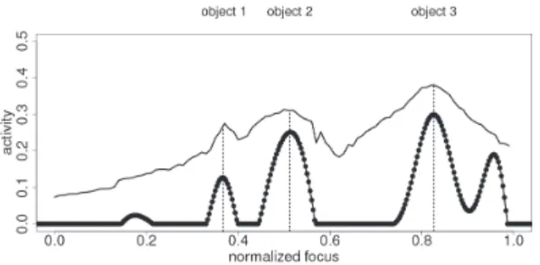
In a third time we focus on the detection of sharpness plans. To do that we used the local standard deviation computed with the points of interest as the input of a Neural-Field. Neural-Fields are dynamic neural networks ruled by two laws: excitation and inhibition (Fig. 10 and [8] for more details). The output of the Neural-Field will show a serie of bumps located at the focus value associated with the different plans of sharpness. Applied to our case it is possible to discriminate the 3 different objects in the scene as shown in figure 9. There is a

Fig. 8:Results of the local standard deviation using the 10-points-of-interest technique. We still see the 3 bumps corresponding to the 3 objects. With this technique the dynamic is larger than with the simple standard deviation computation.

Fig. 9: Results with Neural-Fields. Standard deviation in simple line and Neural-Field activity in dotted line. Instead of the encoders values we preferred a normalized notation for the focus. The bumps of activity are located at focus values linked to the objects. We clearly see the non linearity of the focus-distance relation.

Fig. 10: Left: Description of the neural field rules. The central neurone when activated will excite his close neighbor but inhibit the one further away the inhibition fading out with the distance. Right: Use of the derivative of the neural field activity as the focus control to stabilize it on an object.

problem at the edges of the system due to the discontinuity of the normalized focus space (value only between 0.0 and 1.0). This is partially solved by the use of a circular neural field and adding a inhibition at the edges. The Neural-Field has some friendly properties to address the problem we encounter in our case. It insures that there won’t be any temporal discontinuity in the output signal and also in the focus values. It also helps discriminate the local maxima in the signal by a contrast enhancement and at the same time it merges close sharpness plans in one bump. Finally all those computations are done by a single layer of neurones.

The result can then be used to control the focus and stabilize it on one of the objects. This can be done using different techniques. First fuzzy logic can be used to control the focus. The curve is, in this case, seen as a probability of presence of an object. By using defuzzification techniques the system would be able to stabilize the focus on the plan of sharpness (see [9] for more details).

The output of the neural field can also be seen as basins of attraction. Each object or plan of sharpness creates a basin. By controlling the focus with the derivative of the neural field activity it is possible to stabilize it on an object (Fig. 10). The advantage of this second technique is the possibility to explore the different plans using only the dynamic of the neural field. The focus will be attracted by the closest basin of attraction. This property of bistability is essential to the construction of a stable controller. Given the relation between focus values

and needed zoom correction, it is possible to use the same technique to control the zoom thus insuring the stability of the object size in the vision field.

IV. DISCUSSION ANDCONCLUSION

The system studied here was designed to be as simple as possible. The goal was to explore the options offered by a controllable focus and zoom in order to improve the existing systems in our laboratory.

The global standard deviation was successfully used to obtain a sharp image and by the way the distance to the objects in the scene. With a computation limited to local views centered on points of interest, the dynamic is enhance. The use of Neural-Field to code the data related to the focus allows the system to dynamically stabilize on an object in the scene. Coupled with a pan-tilt system in a similar way as the human eye with head and eye movements, it can provide the necessary information for our objects recognition and navigation systems.

Those where partly described in [10] where Neural-Fields were already and successfully used to find the location of visual clues. We are currently using the focus control to enhance object recognition by scale correction. our recognition system with the scale corrected by the present technique. We are planning on extending its use in manipulation tasks for a humanoid platform. The present system will provide distance and position information for grasping and interaction tasks.

ACKNOWLEDGMENT

This work is part of the project INTERACT (ANR09-COORD014), program CONTINT. (http://interact.ensea.fr)

REFERENCES

[1] S. Gould, J. Arfvidsson, A. Kaehler, B. Sapp, M. Messner, G. Bradski, P. Baumstarck, S. Chung, and A. Y. Ng, “Peripheral-foveal vision for real-time object recognition and tracking in video,” inIJCAI’07: Proceedings of the 20th international joint conference on Artifical intelligence. San Francisco, CA, USA: Morgan Kaufmann Publishers Inc., 2007, pp. 2115–2121.

[2] Y. Y. Schechner and N. Kiryati, “Depth from defocus vs. stereo: How different really are they?”International Journal of Computer Vision, vol. 39, no. 2, pp. 141–162, September 2000.

[3] A. P. Pentland, “A new sense for depth of field,”IEEE Trans. Pattern Anal. Mach. Intell., vol. 9, no. 4, pp. 523–531, July 1987.

[4] N. T. Goldsmith, “Deep focus; a digital image processing technique to produce improved focal depth in light microscopy,”Image Anal Stereol, vol. 19, pp. 163–167, 2000.

[5] J.-V. Leroy, T. Simon, and F. Deschenes, “Real time monocular depth from defocus,” in Image and Signal Processing, ser. Lecture Notes in Computer Science, A. Elmoataz, O. Lezoray, F. Nouboud, and D. Mammass, Eds. Berlin, Heidelberg: Springer Berlin / Heidelberg, 2008, vol. 5099, ch. 12, pp. 103–111–111.

[6] E. Sahin, P. Gaudiano, E. S. Ahin, and P. Gaudiano, “Mobile robot range sensing through visual looming,” in in Proceedings of the ISIC/CIRA/ISAS, 1998, pp. 370–375.

[7] Y.-H. Choi and S.-Y. Oh, “Visual sonar based localization using particle attraction and scattering,” inProceedings of the 2009 IEEE international conference on Mechatronics and Automation, 2005, pp. 449–454. [8] S.-I. Amari, “Dynamics of pattern formation in lateral-inhibition type

neural fields,”Biological Cybernetics, vol. 27, no. 2, pp. 77–87, June 1977.

[9] L. A. Zadeh, “Fuzzy logic,”Computer, vol. 21, pp. 83–93, 1988. [10] S. Leprˆetre, P. Gaussier, and J.-p. Cocquerez, “From navigation to active

object recognition,” inProceedings of the sixth International Conference on Simulation of Adaptive Behavior, 2000, pp. 266–275.