Computational analysis of the biophysical controls on Southern Ocean phytoplankton ecosystem dynamics

COMPUTATIONAL ANALYSIS OF THE BIOPHYSICAL

CONTROLS ON SOUTHERN OCEAN PHYTOPLANKTON

ECOSYSTEM DYNAMICS

by

Tyler W. Rohr

B.S.E., Duke University (2012)

Submitted in partial fulfillment of the requirements for the degree of Doctor of Philosophy

at the

MASSACHUSETTS INSTITUTE OF TECHNOLOGY and the

WOODS HOLE OCEANOGRAPHIC INSTITUTION February 2019

@2019

Tyler W. Rohr. All rights reserved.

The author hereby grants to MIT and WHOI permission to reproduce and to distribute publicly paper and electronic copies of this thesis document in whole or in

part in any medium now known or hereafter created.

Author .

Signature redacted...

...

oint

Program in Oceanography/ Applied Ocean Science & Engineering Massachusetts Institute of Technology & Woods Hole Oceanographic Institution December 19, 2018 Certified by...

S

Certified by. ... Scott Doney Joe D. and Helen J. Kington Professor in Environmental Change University of Virginia Thesis Supervisor

iynature

reUacteU

Wood

Accepted by..

Signature redacted

MASSACHUSETTS INSTITUTE

OF TECHNOLOGY _{Chair, Joint Comm}

I I Mass

...

David Nicholson Associate Scientist s Hole Oceanographic Institution Thesis Supervisor

Shuhei Ono ittee for Chemical Oceanography achusetts Institute of Technology

S ignat1

urerdacted

-COMPUTATIONAL ANALYSIS OF THE BIOPHYSICAL CONTROLS ON SOUTHERN OCEAN PHYTOPLANKTON ECOSYSTEM DYNAMICS

by

Tyler W. Rohr

Submitted to the MIT-WHOI Joint Program in Oceanography and Applied Ocean Science and Engineering on December 19, 2018, in partial fulfillment of the requirements for the degree of Doctor

of Philosophy in Chemical Oceanography

ABSTRACT

Southern Ocean net community productivity plays an out sized role in regulating global bio-geochemical cycling and climate dynamics. The structure of spatial-temporal variability in phytoplankton ecosystem dynamics is largely governed by physical processes but a variety of competing pathways complicate our understanding of how exactly they drive net population growth. Here, I leverage two coupled, 3-dimensional, global, numerical simulations in conjunc-tion with remote sensing data and past observaconjunc-tions, to improve our mechanistic understanding of how physical processes drive biology in the Southern Ocean. In Chapter 2, I show how dif-ferent mechanistic pathways can control population dynamics from the bottom-up (via light, nutrients), as well as the top-down (via grazing pressure). In Chapters 3 and 4, I employ a higher resolution, eddy resolving, integration to explicitly track and examine closed eddy structures and address how they modify biomass at the mesoscale. Chapter 3 considers how simulated eddies drive bottom-up controls on phytoplankton growth and finds that division rates are, on average, amplified in anticyclones and suppressed in cyclones. Anomalous divi-sion rates are predominately fueled by an anomalous vertical iron flux driven by eddy-induced Ekman Pumping. Chapter 4 goes on to describe how anomalous division rates combine with anomalous loss rates to drive anomalous net population growth. Biological rate-based mecha-nisms are then compared to the potential for anomalies to evolve strictly via physical transport (i.e. dilution, stirring, advection). All together, I identify and describe dramatic regional and seasonal variability in when, where, and how different mechanisms drive phytoplankton growth throughout the Southern Ocean. Better understanding this variability has broad implications to our understanding of how oceanic biogeochemisty will respond to, and likely feedback into, a changing climate. Specifically, the uncertainty associated with this variability should temper recent proposals to artificially stimulate net primary production and the biological pump via iron fertilization. In Chapter 5 I argue that Southern Ocean Iron Fertilization fails to meet the basic tenets required for adoption into any regulatory market based framework.

Thesis Supervisor: Scott Doney

Title: Joe D. and Helen J. Kington Professor in Environmental Change University of Virginia

ACKNOWLEDGMENTS

Like all things, an end and a beginning, but now also a sense of time and life catching up with one another. These sort of milestones don't come often, and they certainly don't come alone. Scott, your gentle wisdom and unconditional support have guided me the whole way through. In science, your counsel has always come with a seed of insight and the space to let it grow, and in life, you have been endlessly accommodating to my strange geography. Matt, you consistently provided me with the resources, advice, and collaboration to forge ahead. Hugh, amongst other things, you took me to the end of the world and back. I will never forget how the soft Antarctic dusk would slip seamlessly into the somehow softer light of dawn. It was so beautiful that it barely seemed fair. Steph, you have been kind and insightful throughout, and Roo, you graciously stepped up when I needed someone to co-advise me and you never missed a beat. Finally Cheryl, you more or less adopted me and I couldn't be more fortunate for it. I never enjoy talking about science more than when I'm talking with you. Thank you all. It is both trite and true to say I could not have done it without you.

To all my friends, from TI to GC to JP to LJ, thank you for always being there to indulge my odd fascinations and laugh the ghosts away. You blur the line between community and communion and reiterate the ancient truth that church is really just where ever you find it. That sort of spiritual clarity is a strong elixir for long days or hard years.

Recently, I've begun to find more and more of my church in the mountains. More than anywhere else, the mountains teach me how to feel happy and scarred at the same time. Measured against the hardly justifiable pangs of well-financed millennial anxiety, it can be a quiet miracle to feel brave without wondering if I deserve to. So, it is with immense gratitude and my whole heart when I thank everyone who has ever had the mind to tie in with me. It is a bond that is not soon forgotten. Where ever we have been - in the clouds on Pico Cdo Grande, in the stars on Astroman, below the threat of storms on the Diamond, or above the flight of condors in Patagonia - thank you all for trusting me, and letting me trust you.

It may seem strange, but I would be remiss to not acknowledge the music that has accom-panied, and at times defined, some of the most important pieces of my last half decade. How could I forget listening to Sunday Candy [the Rapper, C., 2016] while cramming with the JP

Chem cohort to keep from going mad, then privately blasting Never Quite Free [Darnielle, J., 2016] in the moments where I thought maybe I had. In Antarctica, and then Patagonia, it was

Jewels, R. T. [20161, Byrne, J. [2016], and XX, T. [20161 shepherding me through my great

Southern Adventure. Last year, it was Ocean, F. [2016], Elverum, P. [2001, 2017] and Wrens,

T. [2003], who kept me afloat in the moments that felt almost impossible. Everywhere else

in between, from the crowded belly of Great Scott (e.g. Planet, D., 2015; Fathers, Y., 2016), to the backroom of a Reykjavik hostel [Baker, J., 2016], to the rain-soaked festival grounds (e.g. House, B. [20161; Vernon, J. [20171), to the old-grove cradle of California [Lekman, J., 2018], a steady drip of live music has brought me joy and shown me grace. And now, as I write this, and ponder the waning hours of a weight being lifting, What It's Like [Russel, A,

Whether you like or not, the wild in you weaves through the wild in me and I wouldn't have it any other way.

And Dad, you taught me how to be proud of this crazy life. Sure, nobody gets it right, but we're all supposed to try, and that can be enough to exercise the things that haunt the hallways of wasted time. You always insisted that whatever I do, I do it with conviction, and then, at the end, you showed me how. For months you cast incantations with a subversive smile against our fears, refusing to give traction to the shape of things to come. Even deep in the trenches, with a head full of tumors, you kept it together. You kept laughing, kept teaching, kept loving, and most spectacularly kept yourself. Before you left, you explained in hopeful gasps that the aperture keeps getting smaller, but the focus stays the same.

This much, at least, is clear: I miss you, I love you, I am from you, and this thesis is, obviously, for you.

The CESM project is supported by the National Science Foundation and the Office of Sci-ence (BER) of the U.S. Department of Energy. Computing resources were provided by the Climate Simulation Laboratory at NCAR's Computational and Information Systems Labora-tory (CISL), sponsored by the National Science Foundation and other agencies. This research was enabled by CISL compute and storage resources. TR was supported by an NDSEG graduate fellowship. TR and SCD acknowledge support from the National Aeronautics and Space Administration Ocean Biology and Biogeochemistry Program (NNX14AL86G). TR, SCD and MTK acknowledge support from the National Science Foundation Polar Programs award 1440435 (Antarctic Integrated System Science) to the Palmer LTER program. Please contact trohrOmit.edu for further questions or to access to data.

CONTENTS

1 Introduction

1.1 M otivation . . . . 1.1.1 Marine primary production, the carbon cycle, and phytoplankton

ecosys-tem dynamics

1.1.2 The Southern Ocean . . . . 1.2 Mechanistic drivers of net population growth and bloom phenology 1.2.1 Mixed layer depth . . . . 1.2.2 E ddies . . . . 1.2.3 Sea Ice . . . . 1.2.4 Human intervention and Ocean Iron Fertilization . . . . 1.3 Observational challenges and the role for models . . . . 1.4 Thesis Overview . . . . . . . . 19 . . . . 20 . . . . 20 . . . . 21 . . . . 22 . . . . 22 . . . . 23 . . . . 24

2 Variability in the mechanisms controlling Southern Ocean phytoplankton bloom phenology in an ocean model and satellite observations 2.1 Introduction . . . . 2.2 M ethods . . . . 2.2.1 Numerical Experiments . . . . 2.2.2 Remote sensing and reanalysis data . . . . 2.2.3 Quantification of relevant rates and metrics . . . . . 2.2.4 Model Skill Metrics . . . . 2.2.5 Regional Bins . . . . 2.3 R esults . . . . 2.3.1 Large-scale Southern Ocean patterns . . . . 2.3.2 CESM Regional Case Studies: Zonal and Latitudinal . . . . . 31 . . . . . 31 . . . . . 33 . . . 33 . . . . . 36 . . . 36 . . . 37 . . . 37 Comparisons . 38 17 18 . . . . 18 27 28

3 Simulated eddy induced bottom-up controls on phytoplankton growth in the Southern Ocean

3.1 Introduction . . . . 3.2 Methods ... ...

3.2.1 Numerical simulation ... ...

3.2.2 Description of diagnostic variables . . . . 3.2.3 Depth extrapolation . . . . 3.2.4 Anomaly and Climatology Fields . . . . 3.2.5 Eddy identification and tracking . . . . 3.2.6 Eddy Subsets . . . . 3.3 R esults . . . . 3.3.1 Simulated and observed eddy track demographics . . . . 3.3.2 Mixing and light limitation . . . . 3.3.3 Iron availability, limitation, and sources . . . . 3.3.4 Anomalous division rates . . . . 3.3.5 Seasonal variability in deep mixing ACC eddies . . . . 3.4 D iscussion . . . .

3.5 3.6

3.4.1 Comparison of theoretical, simulated and observed mixed layer depth anom alies . . . . 3.4.2 Comparison of theoretical, simulated and observed iron transport . . . . 3.4.3 Comparison of theoretical, simulated and observed anomalous division

ra tes . . . . 3.4.4 Basin scale iron budget . . . . C onclusions . . . . Acknowledgments . . . . 57 59 61 61 64 66 67 67 69 70 70 71 72 74 75 75 75 77 78 79 81 81 4 The simulated biological response to Southern Ocean eddies via

rate modification and physical transport

4.1 Introduction . . . . 4.2 M ethods . . . . 4.2.1 Numerical Simulation . . . . 4.2.2 Description of Diagnostic Tracers . . . . 4.2.3 Depth Extrapolation . . . . 4.2.4 Anomaly and climatology Fields . . . .

biological 95 . . . . 97 . . . 100 . . . 100 . . . 102 . . . 105 . . . 105

4.3.1 Rate-based mechanisms . . . . 4.3.2 Physical transport mechanisms . . . . 4.3.3 Spatial and seasonal variability in biomass anomalies . . . . 4.3.4 Depth resolved seasonal variability . . . . 4.4 D iscussion . . . . 4.4.1 Seasonal variability in relative contribution from various mechanisms . . 4.4.2 Comparison of simulated and observed basin scale biomass distributions 4.4.3 Notes on export . . . . 4.5 C onclusions . . . . 4.6 Acknowledgments . . . .

5 Southern Ocean Iron Fertilization: An argument against commercialization but for continued research amidst lingering uncertainty.

5.1 Introduction/Background . . . . 5.2 The case against commercialization . . . . 5.2.1 W ill it work? . . . . 5.2.2 Auditing: Can it be measured? . . . . 5.2.3 Safety: Will it have adverse side effects? . . . . 5.2.4 Managing uncertainty and market failures . . . . 5.3 The case for continued research . . . . 5.3.1 Prospects for commercialization on voluntary offset markets 5.4 Conclusions . . . .

6 Conclusion

6.1 G eneral results . . . . 6.2 Comments on modelling limitations . . . . 6.2.1 Phytoplankton scheme . . . . 6.2.2 Zooplankton scheme . . . . 6.2.3 Sea-ice biogeochemistry . . . . 6.3 Moving forward . . . .

A CESM surface concentration correction model

A .1 Introduction . . . . 107 109 110 111 113 113 116 118 119 120 133 134 136 137 141 142 145 146 146 150 155 156 157 157 159 161 161 165 166

B Supplemental seasonal distributions of climatologies and eddy anomalies

from Chapter 3 171

C Supplemental seasonal distributions of climatologies and eddy anomalies

from Chapter 4 177

LIST OF FIGURES

2-1 Peak bloom size and timing . . . . 2-2 Relative size and timing of simulated depth-integrated phytoplankton specific

grow th rates . . . . 2-3 Regionally averaged, seasonal climatologies simulated by CESM; Al and P1 . . 2-4 Simulated seasonal climatologies of phytoplankton rate and limitation terms;

B in P1 and A l . . . . 2-5 Regionally averaged, seasonal climatologies simulated by CESM; P1, P2, and P3 2-6 Simulated seasonal climatologies of phytoplankton rate and limitation terms;

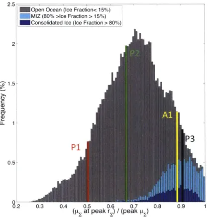
Bin P 1, P2, and P3 . . . . 2-7 Observational and simulated regional climatologies; Bins P1 and Al . . . . 2-8 The frequency distribution of

pat

peakrE . . . .

peakpr,

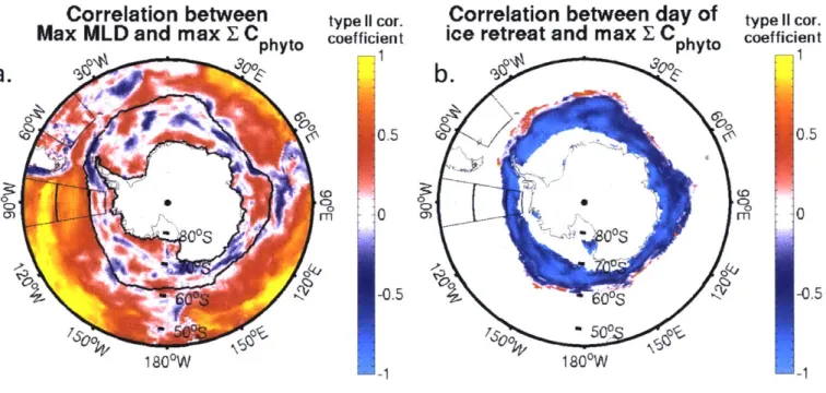
2-9 Simulated bio-physical correlations . . . . Pathways for eddy influence on biomass . . . .

Simulated and observed eddy demographics . . . . Seasonal distribution of eddy tracks and biomass inventory . . . Variability in eddy anomalies . . . . Seasonal MLD climatology and eddy anomalies. . . . . Seasonal [Fe]r climatology and eddy anomalies. . . . . Seasonal Mr, climatology and eddy anomalies. . . . . Vertical iron transport profiles . . . . Sources of anomalous iron . . . . Seasonal variability of eddy anomalies in the deep mixing ACC

4-1 Pathways for eddy influence on biomass

. . . . 82 . . . 83 . . . 84 . . . . 85 . . . 86 . . . . 87 . . . . 88 . . . . 89 . . . . 90 . . . . 91 . . . 121

4-2 Hbvmoller distributions of anomalous biological rate terms in Pacific eddies . . 122 4-3 Variability in rate anomalies as a function of season and background mixed

47 48 49 50 51 52 53 54 55 3-1 3-2 3-3 3-4 3-5 3-6 3-7 3-8 3-9 3-10

4-6 Anomalous biomass flux and concentration associated with vertical transport

m echanism s . . . 126

4-7 H6vmoller distributions of anomalous physical transport mechanisms in Pacific eddies . . . 127

4-8 H6vmoller distributions of anomalous biomass in Pacific eddies . . . 128

4-9 Seasonal variability of depth resolved eddy anomalies in the deep mixing Pacific ACC ... . . .. . . . .. . . ... ... ... ... .. .. . .. .. . .. ..129

4-10 H6vmoller distributions of the correlation between anomalous surface biomass and the underlying mechanisms in Pacific eddies . . 5-1 Ocean iron fertilization schematic . . . . 5-2 Flow Chart: The case against commercialization . . . . . 130

152 153 A-1 COrFacor m odel fit . . . 168

A-2 Time Series of [Cphyto]surf . . . 168

A -3 M odel Skill . . . 169

B-1 Seasonal L PAR climatology and eddy anomalies. . . . 172

B-2 Seasonal L Fe climatology and eddy anomalies. . . . 173

B-3 Seasonal d[e] climatology and eddy anomalies. . . . 174

B-4 Seasonal d[Fe] W climatology and eddy anomalies... . .. .175

B-S Seasonal WEk climatology and eddy anomalies . . . .. 176

C-i Seasonal psE climatology and eddy anomalies . . . . 178

C-2 Seasonal l climatology and eddy anomalies. . . . 179

C-3 Seasonal grE climatology and eddy anomalies. . . . 180

C-4 Seasonal mort climatology and eddy anomalies. . . . 181

C-5 Seasonal aggyr climatology and eddy anomalies. . . . 182

C-6 Seasonal r climatology and eddy anomalies . . . .. 183

C-7 Seasonal Mix,s climatology and eddy anomalies. . . . 184

C-8 Seasonal Wc,s climatology and eddy anomalies . . . . 185

C-9 Seasonal [CPhyto]s STIR climatology and eddy anomalies. . . . 186

C-10 Seasonal [CPhyto]s TRAP climatology and eddy anomalies. . . . 187

C-11 Seasonal [CPhyto]S climatology and eddy anomalies. . . . 188

LIST OF TABLES

3.1 Frequency and magnitude of eddy anomalies . . . . 92

3.2 Spatially averaged anomalous iron supply rate from advection . . . . 93

4.1 Seasonal distribution of frequency of eddies with positive anomalies . . . 131

4.2 Correlation between rate terms . . . 131

4.3 Spatially integrated anomalous biomass . . . 132

CHAPTER 1

1.1

Motivation

1.1.1

Marine primary production, the carbon cycle, and phytoplankton

ecosystem dynamics

Phytoplankton, a broad classification for all autotrophic marine microorganisms, collectively form a vast aquatic forest that stretches across the ocean and helps sustain life on earth. Like terrestrial plants, phytoplankton fix inorganic carbon from carbon dioxide (C02) to form organic carbon compounds and release oxygen molecules (02) in the process as a byproduct. Although phytoplankton only constitute about 1% of global autotrophic biomass, they are responsible for almost 50% of the net primary productivity on the planet [Falkowski et al. 2000]. Marine primary production is in turn responsible for producing half the 02 we breathe [Falkowski et al. 2000] and populating the base of the oceanic food chain which supports the fisheries that millions of people rely on for food [Stock et al. 2017; Watson et al. 2013].

Further, the balance between carbon that is reduced by photosynthesis and oxidized by respiration known as the biological carbon cycle [Riebeek 2011] is responsible for regulating atmospheric C02 levels and climate variability on glacial-interglacial timescales [Berner 1991; Sigman and Boyle 2000]. Variability in the biological carbon cycle is largely driven by marine bioegeochemistry and the biological pump [Berner 1991; Sigman and Boyle 2000], a pathway for medium-to-long term oceanic carbon sequestration [de la Rocha 2006]. Most of the carbon fixed by phytoplankton is rapidly recycled and released back to the atmosphere, but a small fraction

(~

15%) sinks and escapes the euphotic zone where it can remain sequestered in the

deep ocean for hundreds of years before it is reminerialized [Laws et al. 2000].

Although phytoplankton clearly play an integral role in maintaining an oxygen rich at-mosphere, a sustainable food supply, and a stable climate, there remains a great deal of mystery surrounding what controls variability phytoplankton ecosystem dynamics [Falkowski

19971. Unlike terrestrial plants, phytoplankton rapidly turn over their population in a matter

of weeks [Falkowski 2002], making them particularly sensitive to changes in their environ-ment. Moreover, environmental variability is much more dramatic in the ocean than on the land. Physical and biogeochemical processes combine to constantly modify the growth condi-tions and grazing pressure that phytoplankton communities are subject to [Behrenfeld et al.

20131. In turn, net phytoplankton population growth is often limited to short seasonal blooms

[Longhurst 2006] but the mechanisms that shape the size and timing of these blooms highly variable and not fully understood [Rohr et al. 2017].

ecosystem dynamics will help us understand whether or not marine primary production will feedback to buffer or amplify a changing climate, and ultimately how higher trophic levels and fisheries will respond [Chassot et al. 2010]. A variety of mechanisms compete to control phytoplankton ecosystem dynamics [Rohr et al. 2017], complicating our ability to draw direct lines of causality as to how and why blooms form and hampering our ability to predict how a changing environment will modify them. Here, with a focus on the Southern Ocean, I employ a suite of computational methods to study numerical simulations and remote sensing data to help disentangle the biophysical controls on phytoplankton ecosystem dynamics.

1.1.2 The Southern Ocean

Once the crown jewel of human exploration [Elzinga 1993j, by the mid 1900s excitement over the success of the International Geophysical Year had begun to transform Antarctica, and the Southern Ocean writ large, into a cradle for international scientific collaboration [Howkins 2010]. Under protection by the newly established Antarctic Treaty System (ATS), Antarctica was formally codified as a continent for peace and science [Handbook of the Antarctic Treaty

System n.d.]. Since the ATS was ratified in 1959, sweeping interdisciplinary research has

revealed the Southern Ocean as a critical geophysical and biogeochemical node, together acting as a major control on earth's climate system [Turner and Bindschadler 2010].

Geophysically, the Southern Ocean is integral in mixing the global oceans and thereby transporting heat, salt, and nutrients across the world. Laterally, the Antarctic Circumpolar Current is the only substantial connection between earth's major ocean basins [Rintoul et al. 2001] and vertically, deep water formation in coastal polynas plays a critical role in driving global overturning circulation [Marinov et al. 20081. Biogeochemically, Southern Ocean photo-synthetic net community productivity is central to oceanic carbon storage and cycling [ Treguer and Pondaven 2002]. Together, the Southern Ocean is capable of regulating earth's changing climate in a major way [ Watson et al. 20141 and providing a direct feedback into the melting of the Western Antarctic Ice Sheet, which has already begun to lose mass and alone could contribute up 3 meters to global sea level rise [Feldmann and Levermann 2015].

Phytoplankton ecosystem dynamics are particularly interesting in the Southern Ocean. Unlike many ocean basins, phytoplankton division rates are limited by the micro-nutrient Iron, rather than the macro-nutrient Nitrogen [Boyd 2002; Martin et al. 1990]. Further, primary production is often limited by seasonal sea-ice coverage that dims the surface ocean for large portions of the year [Arrigo and van Dijken 2011], and strong grazing pressure by zooplankton

[Hauck et al. 20151, oceanic carbon storage [Marinov et al. 2008] and ultimately global climate

dynamics [Chisholm 2000].

1.2

Mechanistic drivers of net population growth and bloom

phenology

The size [Sullivan et al. 19931 and timing [Racault et al. 2012; Thomalla et al. 2011] of phytoplankton blooms is highly variable across the Southern Ocean. Understanding the role of Southern Ocean phytoplankton dynamics on larger scale biogeochemical and climate cycles is contingent on a better mechanistic understanding of why phytoplankton blooms emerge when and where they do. Phytoplankton bloom dynamics are controlled by a suite of interconnected physical, chemical, and biological mechanisms, which can drive phytoplankton population growth from the bottom-up and top-down. Bottom-up controls refer to anything that affects division rates such as nutrient abundance, light availability, or temperature limitation. In the Southern Ocean the dominant bottom-up controls are light [Nelson and Smith 1991] and iron limitation [Carranza and Gille 2015]. Top-down controls refer to anything that affects loss rates such as grazing, disease, viruses, mortality and aggregation (i.e. sinking). In the Southern Ocean grazing is particularly important [Deppeler and Davidson 2017; Rohr et al. 2017]. Net population growth is driven by subtle differences between two much larger competing rate terms [Behrenfeld et al. 20131. In turn, the size and timing of biomass accumulation, is highly sensitive to a variety of mechanisms that can modify phytoplankton population dynamics both from the bottom-up and top-down. Untangling the influence of these controls, and uncovering where and when certain processes dominate, is instrumental in understanding how marine primary productivity will change in response to the shifting physical landscape of the Southern Ocean [B6ning et al. 2008; Gille 20021.

1.2.1 Mixed layer depth

The predominant bio-physical control on phytoplankton growth is the seasonal mixing cycle, which can include mixed layer depths hundreds of meters deep in Southern Ocean during the winter [Dong et al. 2008]. The classical assumption has held that blooms are light limited, triggered by a shoaling of the mixed layer above some critical level of mean photosynthetically active radiation (PAR), thus eliminating light stress and allowing for high levels of community photosynthesis that exceed losses [Gran and Braarud 1935; Riley 1946; Sverdrup 1953]. This framework emphasizes 'bottom-up' controls, with growth conditions, namely light availability,

critical depth [Behrenfeld 2010; Boss and Behrenfeld 2010; Dale et al. 1999; Townsend et al. 19921 have, however, challenged the canonical association between the mixed layer depth, light limitation, and bloom initiation. For starters, deeper investigations into turbulent mixing rates [Huisman et al. 1999; Taylor and Ferrari 20111 reveal that the mixed layer depth is not always the best proxy for what is actively mixing, calling into question the actual residence time of phytoplankton cycling through the euphotic zone. Moreover, although deep mixing reduces light availability, it also can entrain high concentrations of iron from depth which may be needed to trigger Southern Ocean, iron-limited, blooms [Carranza and Gille 20151. Finally, new evidence has suggested that deep mixing can trigger blooms from the top-down by diluting phytoplankton concentrations and reducing grazing efficiency [Behrenfeld 2010; Behrenfeld et al. 2013]. Behrenfeld et al. [2013] proposed that a bloom can be initiated during deep mixing even if growth conditions are deteriorating from exacerbated light stress, provided that grazing rates are declining even faster as phytoplankton populations are diluted with plankton-free water entrained from depth.

1.2.2 Eddies

The Southern Ocean is characterized by a high degree of mesoscale activity

[Meredith

2016;

Stevens and Killworth 19921 and an abundance of coherent eddy features [Frenger et al. 2015].

Observational [Doney et al. 2003; Large 1998; McGillicuddy et al. 2007] and modeling

[Ander-son et al. 2011; Song et al. 20181 work agree that mesoscale processes help regulate biological

productivity and dominate spatio-temporal variability in phytoplankton distributions [Doney et al. 2003; Glover et al. 2018]. Eddies can influence the biology within them through a vari-ety of, often competing, processes that can both transport biomass and stimulate or suppress biological rates. [McGillicuddy 2016]. From a horizontal perspective, eddies can stir biomass as they rotate [Chelton et al. 2011; Doney et al. 2003; Glover et al. 2018] and trap biomass as they propagate [Early et al. 2011; Flierl 1981; Lehahn et al. 2011]. From a vertical perspective eddies can modify light and nutrient availability by modifying the mixed layer depth through isopycnal displacement [Hausmann et al. 2017; McGillicuddy 2016; Song et al. 2018 and in-duce upwelling or downwelling via eddy pumping [Falkowski et al. 1991; Franks et al. 1986] and eddy-induced Ekman pumping [Dewar and Flierl 1987; Gaube et al. 2014b]. Together, the confluence of various competing mechanisms leads to tremendous spatio-temporal variability in the size and direction of anomalous biomass within eddies [Frenger et al. 2018; Gaube et al. 2014b] and makes it difficult to constrain when and where different mechanisms dominate.

1.2.3

Sea Ice

At high latitudes the introduction of seasonal sea ice can also regulate bloom dynamics. Sea ice imposes severe light limitation during the winter by attenuating incoming solar radiation before it reaches the surface ocean [Arrigo and van Dijken 20111, but also improves light availability during spring by stratifying the water column and reducing the mixed layer depth as it melts [Smith and Comiso 2008; Smith and Nelson 19851. Further, the melt water flux can provide an impulse of nutrients, particularly iron, which can accumulate in the ice over the winter [Fennel et al. 2003; Lancelot et al. 2009; Sedwick and DiTullio 19971. Together, it is not immediately clear if more ice and longer seasonal coverage should be expected to amplify or suppress a bloom, complicating our understanding of what will happen as sea-ice dynamics change [Stammerjohn et al. 2012]. The answer appears to vary with the strength of background wind conditions and the mean annual ice concentration [Montes-Hugo et al.

20091.

1.2.4

Human intervention and Ocean Iron Fertilization

In lieu of a dedicated mitigation effort to combat climate change [Clark 2012; Hovi et al. 2009; Shear 20181, some have suggested that we should use geoengineering to deliberately manipulate the climate system [Lynas 2011]. One proposed method for geoengineering the earth's climate is known as Ocean Iron Fertilization (OIF), which seeks to leverage inefficiencies in Southern Ocean phytoplankton productivity to increase oceanic uptake of atmospheric carbon dioxide

(C02) and thereby sequester anthropogenic carbon for 10-100s of years [Gnanadesikan et al. 20031. The idea is predicated on observations that in the iron-limited Southern Ocean, a relatively small amount of iron can stimulate a large increase in net primary production [Martin and Fitzwater 1988; Yoon et al. 2016]. The hope is that by strategically enriching the Southern Ocean with iron, a rampant increase in productivity could translate into a stronger biological pump, increased carbon exported to depth, and significant long term carbon storage. While, this notion is admittedly seductive, it is hardly advisable. Upper estimates of carbon storage suggest that perfectly efficient OIF could sequester as much as 50-100 ppm C02 [Aumont and Bopp 2006J, but it is unlikely much of the increased productivity stimulated by iron addition would be routed into long term export [Yoon et al. 2016]. Worse, any positive effects would likely be compensated by non-local effects once now macro-nutrient depleted water is upwelled at lower latitudes [Aumont and Bopp 2006; Gnanadesikan et al. 2003; Oschlies et al. 2010; Sarmiento and Orr 19911.

1.3

Observational challenges and the role for models

Relative to its size, the Southern Ocean shoulders a disproportionate role in regulating global biogeochemical [Marinov et al. 2008] and climate cycles [Chisholm 2000], yet remains largely understudied relative to lower latitude ocean basins. This stems directly from a host of chal-lenges that befuddle traditional observational platforms [Abrahamsen 2014]. Harsh conditions characterized by high seas and strong storms coupled to remote locations far from support reduce the opportunity for shipboard observations throughout the year. Without major ship-ping lanes it is not possible to put passive monitoring equipment on commercial vessels and targeted oceanographic expeditions are much more logistically and financially demanding. In the winter, heavy sea ice coverage typically prevents shipboard observations altogether, leaving a massive seasonal hole in observations. The recent proliferation of ARGO floats [Gould et al. 2004] and drifters (e.g. Webb et al. [20011) has begun to fill in the gaps but most floats and drifters are still subject to many of the same constraints, such as the inability to surface under ice. To date, the best bet to observe the Southern Ocean has been from space, nevertheless, satellite-based remote sensing observations are also constrained by their own set of challenges

and limitations, particularly at high latitudes.

For starters, several factors work to blind satellite sensors from the oceans surface. Sea-sonal sea ice, cloud cover, and the positioning of the sun all work to prevent satellites from seeing the surface ocean, especially during the winter when ice and clouds are abundant and long nights combined with a sharp solar zenith angle at high latitudes keep satellites in the dark [Dierssen and Smith 2000]. Even when satellites can see the surface ocean unobstructed, there are limitations regarding what can be inferred about the biological system [Xavier et al. 2016]. Ocean color, observable passively from space, provides a reliable proxy for chloro-phyll concentrations, but fails to consider variability in particle size distributions [Dierssen and Smith 2000], photo-acclimation [Sakshaug and Holm-Hansen 1986], or community com-position, which all can change the chlorophyll to carbon ratio and bias estimates of biomass inferred from chlorophyll [Dierssen and Smith 2000]. More recently, direct estimates of carbon biomass have been made from particle back-scattering and absorption coefficients using the GSM spectral matching algorithm [Garver and Siegel 1997] and the carbon based productiv-ity model [Behrenfeld et al. 2005; Westberry et al. 2008], however these are subject to their own set of biases and assumptions and have not yet been tested as thoroughly against in-situ observation as other chlorophyll-based products (e.g. Saba et al. [2011]).

by extrapolating surface concentrations over the mixed layer depth, but estimations of the mixed layer depth can not be observed remotely. In-situ observations have become more prevalent, but local data must be stitched together using state estimates (e.g. Mazloff et al. [2010]) or re-analysis products (e.g. Milutinovid et al. [2009]), that are likely to miss much of the high frequency variability in seasonal and spatial mixing dynamics. Moreover, even once a mixed layer estimation is established, it is still often problematic to assume biomass is distributed uniformly across it. Results can be biased by biomass below a shallow mixed layer

[Behrenfeld et al. 2013], nonuniform biomass profiles and/or subsurface maxima [McGillicuddy

et al. 2007; Siegel et al. 19991.

While observations are obviously foundational to our understanding of the Southern Ocean, the challenges detailed above limit their capacity to fully constrain Southern Ocean biogeo-chemical cycling and phytoplankton ecosystem dynamics, especially during the winter and at depth. In turn, many have pointed to the need to leverage numerical models to simulate what can not be observed (e.g. Frenger et al. [20181 and Gaube et al. [2014a]). Models, of course, can never perfectly describe nature and are limited by the processes and scales that are resolved. Nevertheless, numerical simulations are valuable in their ability to fill in gaps in the observational record, make predictions, and explicitly resolve the processes and mechanisms that can not be directly observed. In turn, models are clearly a necessary to compliment incomplete observations but must be tempered with an understanding of what is prescribed, parameterized and able to be resolved at the resolution of a particular integration. As the skill of coupled general circulations models continues to evolve in parallel with advances in the computing capacity needed to power them and the observational understanding needed to inform them, numerical simulations and broader computational methods will only become an increasingly important piece of Southern Ocean biogeochemical research.

1.4

Thesis Overview

Here, the state of the art Community Earth System Model (CESM) is used in conjunction with observations to help disentangle the controls on Southern Ocean phytoplankton ecosys-tem dynamics. First, in Chapter 2 the relative roles of bottom-up controls (division rates) and top-down controls (grazing rates) are examined in the context of net population growth rates and bloom phenology across the Southern Ocean. Results, simulated explicitly and sup-ported by observations, demonstrate that blooms can be triggered by a variety of mechanisms, including mixed layer shoaling, mixed layer deepening, and sea ice retreat. Moreover, blooms

ulate or suppress the division rates of phytoplankton populations within them are examined. Results find that simulated eddies amplify divisions rates in Southern Ocean anticyclones, pri-marily by transporting iron from depth via eddy-induced Ekman Pumping. The opposite was found in cyclones. Next, in Chapter 4 the relative effects of eddy modified division rates, loss rates, net population growth rates, and physical transport mechanisms are all considered in the context of the biomass anomalies they combine to create. Different mechanisms are found to dominate at different times and different places, leading to tremendous spatio-temporal variability in the size and direction of eddy-induced biomass anomalies across the Southern Ocean. In Chapter 5 the merits of Ocean Iron Fertilization (OIF) are considered in light of the established complexity associated with the mechanistic underpinning of Southern Ocean phytoplankton blooms. An extensive review of the best-available science, international pol-icy framework, and developing market forces confirms that lingering uncertainty coupled to concerns over efficacy, safety, and measurement prohibit a viable commercialization strategy. Finally, conclusions and future directions are presented in Chapter 6.

CHAPTER 2

VARIABILITY IN THE MECHANISMS CONTROLLING

SOUTHERN OCEAN PHYTOPLANKTON BLOOM

PHENOLOGY IN AN OCEAN MODEL AND SATELLITE

Abstract

A coupled global numerical simulation (conducted with the Community Earth System Model) is used in conjunction with satellite remote sensing observations to examine the role of top-down (grazing pressure) and bottom-up (light, nutrients) controls on marine phytoplankton bloom dynamics in the Southern Ocean. Phytoplankton seasonal phenology is evaluated in the context of the recently proposed 'disturbance-recovery' hypothesis relative to more tra-ditional, exclusively 'bottom-up' frameworks. All blooms occur when phytoplankton division rates exceed loss rates to permit sustained net population growth, however the nature of this decoupling period varies regionally in CESM. Regional case studies illustrate how unique path-ways allow blooms to emerge despite very poor division rates or very strong grazing rates. In the Subantarctic, southeast Pacific small spring blooms initiate early co-occurring with deep mixing and low division rates, consistent with the 'disturbance-recovery' hypothesis. Similar systematics are present in the Subantarctic, southwest Atlantic during the spring, but are eclipsed by a subsequent, larger summer bloom that is coincident with shallow mixing and the annual maximum in division rates, consistent with a 'bottom-up', light limited framework. In the model simulation, increased iron stress prevents a similar summer bloom in the southeast Pacific. In the simulated Antarctic zone (70'S - 65'S) seasonal sea-ice acts as a dominant phytoplankton-zooplankton decoupling agent, triggering a delayed but substantial bloom as ice recedes. Satellite ocean color remote sensing and ocean physical reanalysis products do not precisely match model predicted phenology, but observed patterns do indicate regional variability in mechanism across the Atlantic and Pacific.

Key Points

" CESM explicitly simulates variable pathways for Southern Ocean bloom formation driven by both bottom-up and top-down controls

" Simulated blooms can initiate amidst both strong or poor cell division rates depending on iron/light availability and trophic decoupling

" Implicit evidence in the remote sensing data supports these unique mechanistic pathways as well as a strong but variable grazing control

carbon cycling [Siegel et al. 20141 and thus global climate dynamics [Chisholm 2000; Trdguer and Pondaven 20021. In the SO, iron limitation [Boyd 2002; Martin et al. 1990], seasonal sea-ice cover [Arrigo and van Dijken 20111 and trophic dynamics constrain the net population growth of phytoplankton to seasonal blooms [Longhurst 2006]. Understanding these seasonal cycles in phytoplankton ecosystem dynamics is critical to our understanding of spatial and temporal variability in Southern Ocean NCP but is hampered by the complexity of intercon-nected physical, chemical, and biological controls.

Phytoplankton bloom dynamics are governed by bottom-up factors that control cell di-vision rates, as well as top-down factors that control grazing and other loss rates. The net effect on seasonal net population growth is a balance between a number of different, and often opposing, bottom-up and top-down factors, and as a result, the timing of bloom initiation can vary substantially geographically and from year to year.

From a bottom-up perspective, light limitation can suppress division rates during deep winter mixing when depth averaged photosynthetically active radiation (PAR) over the mixed layer is low. For a bloom to occur, the springtime mixed layer depth must shoal above some critical level for depth-averaged PAR to drive levels of community photosynthesis above losses

[Gran and Braarud 1935; Riley 1946; Sverdrup 1953]. In this context, phytoplankton biomass

concentration is assumed to be well coupled to the depth-integrated inventory, and bloom ini-tiation is typically estimated as the point in time when surface concentrations begin to increase substantially [Siegel et al. 2002]. However, some observations indicate that depth integrated biomass can increase before the mixed layer shoaled above this critical depth [Dale et al. 1999;

Ellertsen 1993; Townsend et al. 19921 implying that bloom inception may be influenced by

other mechanisms including dilution (or disturbance)-recovery [Fischer et al. 2014]. Mixed layer deepening can mediate 'top-down' controls on bloom development [Behrenfeld 2010;

Behrenfeld et al. 2013] and decouple concentration-based and inventory-based growth rates.

Bloom initiation, instead defined as the switch to positive net growth of the column-integrated population rather than surface concentration, can be triggered by subtle disequilibria in trophic coupling that decrease predation by zooplankton and promote sustained increases in phyto-plankton biomass integrated over the mixed layer. This disequilibrium is modulated, in part, by entrainment during the fall and winter of phytoplankton depleted water during deep mix-ing, diluting the phytoplankton concentration on which grazing rates depend. Since grazing scales with prey concentrations, dilution can cause loss rates to drop below division rates; thus, deep mixing can actually maintain (or increase) the vertically integrated phytoplankton inven-tory [Behrenfeld 2010; Behrenfeld et al. 2013]. Under this 'disturbance-recovery' framework,

From a bottom-up perspective, deep mixing can also entrain nutrients from depth, replen-ishing surface levels of macro- and micronutrients [Carranza and Gille 20151, which are known to limit net primary productivity [Moore et al. 2013b]. In particular, throughout the Southern Ocean, iron is largely thought to be the dominant limiting nutrient, leading to expansive High Nitrate, Low Chlorophyll (HNLC) regions [Boyd and Ellwood 2010; de Baar et al. 1995, 2005;

Martin et al. 1990]. However, the degree of iron limitation across the Southern Ocean is quite

variable in space and time. Regional inputs from atmospheric dust deposition, anoxic coastal sediments, river runoff, and sea/glacial ice provide exogenous iron sources of varying signifi-cance [Boyd et al. 2012; Moore and Braucher 2008] that can modify bloom size and duration, and regulate the importance of deep mixing as an iron source.

Sea-ice can both hinder high latitude bloom development through severe surface light lim-itation [Arrigo and van Dijken 2011] and support cell division following ice melt via increased vertical stratification [Smith and Comiso 2008; Smith and Nelson 1985] and nutrient enrich-ment (particularly Fe) [Fennel et al. 2003; Lancelot et al. 2009; Sedwick and DiTullio 1997]. Note, however, nutrient enrichment from ice melt is not incorporated into many global-scale ocean biogeochemical models including the one used in this analysis (see 2.2.1). As South-ern Ocean sea-ice dynamics are modified by climate change [Stammerjohn et al. 2012] these competing processes can lead to dramatically different effects on bloom dynamics. Depending on regional wind conditions and total ice concentration, decreased sea-ice could dampen or amplify the bloom [Montes-Hugo et al. 20091.

This complex suite of controls drives variability in the size [Moore and Abbott 2000; Sullivan et al. 1993] and timing [Racault et al. 2012; Thomalla et al. 2011] of phytoplankton blooms, which can affect trophic transfer and carbon export. Disentangling these controls is critical in understanding present, and predicting future, spatio-temporal variability in Southern Ocean NCP, and ultimately the role of marine autotrophs in a changing climate. In this study, model results and remote sensing observations are used to showcase how physical and biogeochemical controls can produce blooms via different mechanisms. In doing so, we test the suitability of the 'disturbance-recovery' hypothesis relative to more traditional, strictly 'bottom-up' systematics.

We first highlight the observed and simulated spatial variability in bloom size and timing across the Southern Ocean (see 2.3.1). Next we analyze how well coupled peak cell division rates are to peak net population growth rates and peak biomass inventory within the model to help infer the strength of bottom-up controls (see 2.3.1). Different mechanistic pathways are then explicitly examined by comparing the simulated climatologies of the relevant physics and biogeochemistry for four spatially averaged regional case studies simulated in CESM (see

2.2

Methods

2.2.1

Numerical Experiments

The Community Earth System Model (CESM) is a fully coupled, global climate model capable of simulating past, present, and future climate scenarios [Hurrell et al. 20131. Here we utilize a preindustrial simulation with a recently improved treatment of photosynthesis under sea-ice [Long et al. 2015]. The new treatment better represents the effect of subgrid-scale heterogeneity in sea-ice thickness and water column irradiance on the non-linear (concave downward [Geider et al. 1998]) photosynthesis-irradiance curve, leading to a more realistic phenology and bloom magnitude. This 30-year simulation has been branched off a longer control simulation, and most model output was saved at high temporal resolution as daily means.

Except for the new sea-ice treatment, the component set up is identical to that of the

1850 control used in the CESM Large Ensemble project and described in detail by Kay et

al. [2014]. The ocean component has nominal horizontal resolution of

1

degree and 10m vertical grid cells down to 250m. Sea-ice is treated using the CICE4 component [Hunke and Lipscomb 20081. The ice model does not sequester iron or resolve any biogeochemistry. All atmospheric dust deposition over sea-ice is deposited directly into the surface water. The ocean biogeochemistry component (BEC) detailed by [Moore et al. 2013a] has been tested and validated against global datasets and shown to capture basin-scale spatial distributions in production, nutrient and chlorophyll concentrations [Doney et al. 2009; Moore et al. 2004, 2013a; Moore et al. 2013b], and key aspects of oceanic iron [Moore and Braucher 2008] and carbon cycling [Lima et al. 2014; Long et al. 2013; Moore et al. 2013a]. BEC features a single class of zooplankton and three phytoplankton functional types: diatoms, small phytoplankton, and diazotrophs. Diazotrophs, however, are strongly limited by temperature and therefore exist only in negligible concentrations in the Southern Ocean. Phytoplankton carbon biomass,

Cphyto(mmol C), is tracked in terms of grid cell concentration, [Cphyto](mmol C m-3).

Phytoplankton net population growth (ld[Cp, yt]) is governed by a photosynthetic net primary productivity term, Pphyto, and opposed by losses due to a grazing, Gphyto, linear mortality,

mortphyto, and quadratic mortality/aggregation, aggphyto, term, such that,

d[ChYntO]-dt po -

Gphyto

- G -hyt - mortphyto - aggphyto, (2.1)

where all terms are in ( "9 "C) and phyto represents either of the two regionally dominant pools of autotrophic plankton resolved in the simulation, diatoms or small phytoplankton.

(N, P, Si, Fe) limitation (L') and light availability (LIPAR). Individual nutrient limitation terms vary from 0 to 1 as a nonlinear function of the available nutrient concentration and a class-specific nutrient specific half saturation coefficient. Multi-nutrient limitation is treated following Liebig's Law of the minimum [van der Ploeg et al. 1999] such that the maximum spe-cific photosynthetic division rate (Ap,'to) is only scaled by the most limiting nutrient limitation term rather than a multiplicative function of each. Note that because the nutrient limitation term scales the maximum growth rate lower values translate to greater nutrient stress. Nu-trient stress is systematically less for small phytoplankton than for diatoms given the same nutrient concentration because of differences in the parameterization of their respective half saturation coefficients chosen to account for differences in their size and physiology [Sunda and

Huntsman 19951. Light limitation (LIPAR) scales as a nonlinear function of photosynthetically

available radiation, a dynamic Chl : C ratio and the most constraining nutrient limitation term. Both the Chl : C ratio and nutrient limitation terms are computed differentially for individual phytoplankton pools resulting in a species specific light limitation term. Together,

a= LTnLIPAR (2.2)

Grazing occurs on individual phytoplankton pools and is governed by a temperature depen-dent, non-linear function (Holling type III; [Holling 1959]) of the phytoplankton concentration such that,

Gphmto = .rnaxLT( _[Cphyto]2

_)[Zcl,

(2.3)

[Cphyto] yto

where oohyt(d-') is the maximum zooplankton specific grazing rate on phytoplankton class phyto, LT is the dimensionless temperature dependency term, [Cphytol is the class-specific phytoplankton carbon concentration (mmol C m 3), gphyto is the zooplankton class-specific grazing coefficient (mmol C m-3), and

[Zc]

is the zooplankton carbon biomass concentration

(mmol C m-3). The class specification of the grazing parameterization ensures that

zooplank-ton are more effective grazers on the small phytoplankzooplank-ton class, affording a relatively complex trophic control on phytoplankton at an affordable computational cost. Zooplankton is in turn governed by differential grazing on all three phytoplankton populations weighted by a non-dimensional ingestion coefficient and a temperature dependent loss term. The nonlinearities of the grazing equation ensure that zooplankton become more efficient grazers as phytoplankton concentrations increase, eventually saturating towards a maximum grazing rate.

2.2.2

Remote sensing and reanalysis data

We analyze ocean color remote sensing records compiled at 8-day resolution from 2005-2014 from the MODIS/Aqua satellite program. Observational indicators of phytoplankton abun-dance and growth include MODIS surface chlorophyll records, as well as phytoplankton carbon biomass and cell division rates estimated from particle back-scattering and absorption coeffi-cients using the GSM spectral matching algorithm [Garver and Siegel 1997] and the carbon based productivity model (CbPM) outlined by Behrenfeld et al. [2005] and later improved and validated against global data sets by Westberry et al. [2008]. Observationally-based mixed layer depth estimates are sourced from HYCOM and FNMOC reanalysis projects [Milutinovid et al. 2009]. HYCOM and FNMOC data sets are merged for improved spatial and temporal cov-erage. All aforementioned data has been sourced from the Oregon State Ocean Productivity web page [O'Malley 2015]. Daily sea-ice fractional coverage is estimated at 25km resolution using the GSFC Bootstrap SMMR-SSM/I Version 2 time series [Comiso 2011; Comiso et al.

1997; Shang et al. 2010].

2.2.3 Quantification of relevant rates and metrics Phytoplankton metrics

All modeled phytoplankton metrics (unless otherwise noted) are calculated for the sum of the two regionally dominant phytoplankton functional types, small phytoplankton and diatoms (See 2.2.1). CESM resolves both carbon and chlorophyll concentrations for each phyoto-plakton pool using a dynamic Chl:C ratio to account for photoacclimation. In our analysis, phytoplankton abundance is quantified in carbon units (as opposed to chlorophyll) to avoid biases introduced by photoacclimiation. Note, however, that phytoplankton chlorophyll and carbon biomass have been shown to be well correlated in the Southern Ocean [Arrigo et al. 2008; Behrenfeld et al. 2005; Qu6r6 et al. 2002]. To first order, qualitatively similar patterns in bloom size and timing appear in biomass estimated from the CbPM (see Fig. 2-1) and chloro-phyll as observed by MODIS as well as the Coastal Zone Color Scanner and SeaWiFS [Moore and Abbott 2000; Sullivan et al. 1993]. During strong dilution events, however, it is possible that chlorophyll-based metrics will overestimate biomass as low light and photoacclimation increase the Chl:C ratio

Daily modeled and observed [Chlphyto]surf values are used in our diagnostic analysis to approximate the euphotic depth following the empirical relationship developed by [Morel and

Model simulated, depth resolved profiles of [Cphyto] were only saved as monthly means, and therefore exact values of phytoplankton carbon inventory (ECphyto) integrated to time-varying mixed layer depth or euphotic depth can only be computed from monthly averages of biomass and depth. However, daily-mean simulated values are available for the phytoplankton carbon inventory integrated over the upper 100m of the water column ( EC100 mmolCm 2 ).

Assumptions regarding the vertical distribution of biomass allow us to approximate both daily total water column inventory and surface concentrations. Following Behrenfeld et al. [2013], we assume that phytoplankton biomass is homogenously distributed across the greater of the mixed layer depth or euphotic depth (Zeu), referred to as the Profile Depth, Zprofile =

max(MLD, Zeu). Biomass is assumed to drop to 0 below this depth. This assumption holds

well for an actively mixing mixed layer that is deeper than the euphotic depth, though could be problematic for shallow mixed layers where phytoplankton biomass can persist in stratified water below the mixed layer depth [Behrenfeld et al. 2013; Boss and Behrenfeld 2010; Boss et al. 2008] or when there is little active mixing [Franks et al., 2015]. Specifically in the Southern Ocean, [ Uitz et al. 2006] concluded from in-situ data sets that it was reasonable to assume a uniform distribution in deep, well-mixed water.

The water column phytoplankton carbon inventory is thus assumed equal to the vertical

Zprofile

integral over Zprofile (E-Cphyto = fIurface [Cphyto]dZ, mmol C r-2_{). For the model analysis,} we use the daily-mean 100m integral to approximate the inventory (ECphyto = EC'oo) when

Zprofile < 100m, recognizing that non-zero biomass in the depth range Zprofile - 100m may

violate our distribution assumption; however this assumption does not bias our approximation of total water column inventory. Additional biomass below 100m is unaccounted for but unlikely to be significant given a shallow Zprofile. When Zprofile > 100m we extrapolate from 100m to Zprofile using the mean 0 - 10m concentration (ECphyto = (Zpr" EC1 0)).

Here the assumption of a uniform profile is reasonable, particularly in CESM, given a deep, well-mixed layer that likely exceeds the euphotic depth.

Modeled surface carbon biomass concentrations ([Cphyto] surf, mmol m- 3) also were saved

only as monthly means. Daily surface concentrations are first approximated by assuming a uniform depth profile across Zprofile and dividing inventory by profile depth ([Cphyto]snrf =

ECphyto/Zprofile

).

This approximation can be problematic for shallow mixed layers where

biomass may exist in the euphotic zone below the mixed layer depth. To improve our first approximation for shallow profiles (Zprofile < 100m), estimated surface concentrations are further weighted by a spatially and profile depth dependent correction factor modeled from the simulated monthly surface concentration data (see Appendix A.1-A.3). Testing the skill

Remote sensing observations provide only surface concentrations, which are extrapolated to ZPrOfile following [Behrenfeld et al. 2013], under the same uniform depth distribution as-sumption.

Volumetric phytoplankton specific net population growth rates, r (d- 1), can be related to

the specific photosynthetic division rate, p (d-1), by

1

d[Cphto _ _(2.4)

[Cphyto] dt

where 1 (d-) is the total specific loss rate composed of grazing (lGr, phyto) , phytoplankton mortality (1mort, phyto), and aggregation (lagg, phyto) (see Eq. 2.1). Volumetric specific rate terms (p, 1) for a grid cell are calculated by normalizing the rate terms as they appear in Eq.

2.1 by the biomass concentration (p = Ul '0 - _ __ iGr,phyto+Imort,phyto+lagg,phyto

[Cphyto] [Cphyto]

Vertically-integrated population specific rates (pE, 1>i,Gr,phyto, E,>mort,phyto, 1Eagg,phyto d-1)

are calculated by dividing the water column integrated daily rate terms (EPphyto, EGrphyto,

Emortyhyto, Eaggphyto; mmol C m-2d-1 ) by the depth integrated phytoplankton carbon

in-ventory (ECphyto). The total population specific loss rate (l) is the sum of its components

= EGr,phyto + lEmort,phyto +

lagg,phyto)-In the model, rate terms (Pphyto, Gryhyto, mortpahto, aggphyto) are saved as daily mean 150m depth resolved profiles. If Zprofile > 150m, we assume that rates(z > 150m) = rates(z 150m).The population specific net growth rate for the depth-integrated inventory, r( can thus be explicitly calculated as

rE = uE - ly (2.5)

Without explicitly resolved rate terms, in the remote sensing data rE (d-'), between two time points, t=0 and t=1, is calculated from temporal changes in phytoplankton biomass as follows,

rE= Iin(ECphyto_1/ECphytoo)/At, if MLD is deepening and > Zeu (2.6)

rr = ln([Cphyto-1]ssrf /[Cphyto-O]surf)/At, if MLD is shoaling or < Zeu (2.7) where either concentration or vertical inventory is used, depending on mixed layer dynamics, to take into account dilution effects by entrainment of phytoplankton free water from below during deep mixed layer deepening. Bloom initiation is in turn defined as the onset of positive