Modeling the Luminance Degradation of OLEDs using Design of Experiments (DoE)

HAL Id: hal-02465792

https://hal.archives-ouvertes.fr/hal-02465792

Submitted on 4 Feb 2020

HAL is a multi-disciplinary open access

archive for the deposit and dissemination of

sci-entific research documents, whether they are

pub-lished or not. The documents may come from

teaching and research institutions in France or

abroad, or from public or private research centers.

L’archive ouverte pluridisciplinaire HAL, est

destinée au dépôt et à la diffusion de documents

scientifiques de niveau recherche, publiés ou non,

émanant des établissements d’enseignement et de

recherche français ou étrangers, des laboratoires

publics ou privés.

Modeling the Luminance Degradation of OLEDs using

Design of Experiments (DoE)

Farah Salameh, Andrea Al Haddad, Antoine Picot, Laurent Canale, Georges

Zissis, Marie Chabert, Pascal Maussion

To cite this version:

Farah Salameh, Andrea Al Haddad, Antoine Picot, Laurent Canale, Georges Zissis, et al.. Modeling

the Luminance Degradation of OLEDs using Design of Experiments (DoE). IEEE Transactions on

Industry Applications, Institute of Electrical and Electronics Engineers, 2019, 55 (6), pp.6548 -6558.

�10.1109/TIA.2019.2929150�. �hal-02465792�

OATAO is an open access repository that collects the work of Toulouse

researchers and makes it freely available over the web where possible

Any correspondence concerning this service should be sent

to the repository administrator:

tech-oatao@listes-diff.inp-toulouse.fr

This is author’s version published in:

http://oatao.univ-toulouse.fr/25251

To cite this version:

Salameh, Farah and Al Haddad, Andrea and Picot, Antoine

and Canale, Laurent and Zissis, Georges and Chabert, Marie

and Maussion, Pascal Modeling the Luminance Degradation

of OLEDs using Design of Experiments (DoE). (2019) IEEE

Transactions on Industry Applications, 55 (6). 6548 -6558.

ISSN 0093-9994.

Official URL:

https://doi.org/10.1109/TIA.2019.2929150

Modeling the Luminance Degradation of OLEDs using Design of Experiments (DoE)

Farah

Salameh

LAPLACE, Université de Toulouse, CNRS, INPT, UPS, Toulouse, France. farah-salameh@live .com

Andrea

Al Haddad

LAPLACE, Université de Toulouse, CNRS, INPT, UPS, Toulouse, France alhaddad@lapla ce.univ-tlse fr

Antoine

Picot

LAPLACE, Université de Toulouse, CNRS, INPT, UPS, Toulouse, France picot@laplace. univ-tlse fr

Laurent

Canale

LAPLACE, Université de Toulouse, CNRS, INPT, UPS, Toulouse, France canale@laplac e.univ-tlse.fr

Georges

Zissis,

LAPLACE, Université de Toulouse, CNRS, INPT, UPS, Toulouse, France zissis@laplace .univ-tlse fr

Marie

Chabert

IRIT, Université de Toulouse, CNRS, INPT, UPS, Toulouse, France. marie.chabert @enseeiht fr

Pascal

Maussion

LAPLACE, Université de Toulouse, CNRS, INPT, UPS, Toulouse, France maussion@lap lace.univ-tlse fr

Abstract -- Modeling the lifespan of OLED (Organic

Light-Emitting Diode) is a complex task as it depends on different - potentially interacting factors. As the literature on this subject is still scant, new parametric models for calculating the lifespan of OLED are proposed in this work. The Design of Experiment (DoE) methodology is used for cost and accuracy reasons. Different lifespan models based on thermal and electrical experimental aging tests are proposed. As stress factors, current density, temperature and their interactions, which are rarely taken into account in aging studies are simultaneously involved. The analysis of the model parameters highlights the prevalence of temperature compared to current density on the luminance performance of OLEDs. Non-linear models appear as the most accurate.

Keywords -- accelerated aging, design of experiments, electrical

stress, lifespan prediction, OLED, thermal stress I. INTRODUCTION

Nowadays, system and component reliability has become an important issue. A clear understanding, modeling and predicting aging and degradation mechanisms could lead to upgrade the quality and the reliability of the components and avoid system failure. The operational constraints (supply, atmospheric, mechanic, etc.) and their effects on the degradation of components must be studied to predict the lifespan and find solutions to improve the reliability. In the field of electrical engineering, numerous lifespan models have been developed in the literature [1]-[4] but these models present some limitations. Indeed, they depend on the studied material and on its physical properties and they are often restricted or focused to one or two stress factors. Moreover, they do not integrate interactions that may exist between these different factors. The future of light sources will be probably leads by SSL (Solid State Lighting) i.e. LEDs and OLEDs, but those last have a limited lifespan (30,000h to 40,000h) and an aging mode that is still largely unknown. Although this methodology is general and applicable to various components with no prior information on their physical properties, the measurement specifications have to

take into account in order to compute a relevant lifespan model.

This paper presents an innovative parametric lifespan models for very recent OLED light sources which the aging characteristics are still largely unknown. The proposed models are inferred from the experimental data obtained through accelerated aging tests involving several stress factors are used to infer the proposed models. Those are innovative because they take into account, not only the effects of the different stress factors, but also, at the same time, their possible interactions. This is rarely done in aging studies. This kind of predictive models is perfectly adapted in studies where there is few and/or expensive samples. Moreover, this methodology allows to maximize the model accuracy with a small learning sets composed by an optimized number and appropriate configuration of experiments in order to reduce the number and the cost of experiments. The significance of the considered parameters onto the stress factors is assesses by a study of the parameters inputs at different lifespan levels. OLED degradations could be leads by two ways: intrinsic and/or extrinsic factors [5]. The first case is related at moisture or oxygen that can induce delamination or oxidation of the electrodes and can generate dark spots. This can be avoided by a good encapsulation. Extrinsic degradations are mainly leading by the supply current and the ambient temperature where this last is considered as the most impacting factor of degradation [6][7]. Depending on the threshold, the temperature can contribute to the OLEDs degradations during use but can also, in the case of high temperature, contribute to degradations during storage [8]. OLEDs are current-controlled components where their luminance is proportional to the supply current level [8]. But the forward current is also the second main degradation factor. Due to the chemical degradation of the organic materials by the flowing current through the layers, their performances decrease gradually over time [9]. The chosen OLED in this work are commercial products and present two

great advantages: they are well encapsulated and show a great repeatability. A good encapsulation can prevent against oxygen and moisture factors, and it allows us to focus our study only on extrinsic degradations. Thus, thermal and electrical stresses remain the most critical degradation factors for OLEDs. When OLEDs are used for lighting applications, the luminance (measured in cd/m²) is, obviously, the most interesting output parameter and also a simple feature to be monitored. The degradation of an OLED is defined by the decay of its luminance over time [10]. It is commonly assumed that the end of life of an OLED is when the luminance degrades by 30% to 50% depending on the application. The corresponding lifetimes are therefore mentioned L70 or L50, corresponding of a decay from the initial value of 30% and 50%, respectively. To date, there is no standard measurement method for OLEDs light source that can be adopted in performance or accelerated aging tests [8], [11]. Some standards and recommendations has been published (as a US standard, in September 2013 [12] that specifies the general safety conditions for the use of OLED lighting panels and an international IEC standard in 2014 [13] about the safety requirements) but the international standard IEC 62922, concerning the evaluation of the performance and reliability of OLEDs, has still not been published.

II. EXISTING METHODS FOR AGING MODELING

In the OLED aging literature, the thermal and electrical characteristics of different physical composition OLEDs have been studied to evaluate its thermal degradation [15]. Nevertheless, no modeling is done. Another aging sign for the OLEDs is its luminance degradation. Many articles use this sign as a lifespan indicator. In order to achieve this degradation, most papers use accelerated lifetime tests. The magnitude of stresses, in this case, is much bigger than nominal conditions. Park et al. [10] used accelerated degradation tests to study OLED lifetime. They proposed distribution-based lifespan models (lifetime following Weibull, lognormal, log-spline functions …) along with other methods to study the effect of thermal stress on the aging. Like the previous paper, [14] studied the effect of thermal stress on the accelerated degradation of phosphorescent OLED. It estimated their Mean Time To Failure (MTTF) under normal conditions using a Weibull function for the lifetime distribution and an acceleration factor. Other papers studied the effect of current density on the OLED aging. In [11], the authors suggested that the lifetime is a “power function” of current by plotting the measured lifespans as a function of the applied current. They used this model to characterize OLED panels. A Weibull distribution to model the OLEDs lifespan under constant step current density stresses was proposed in [18] and the same authors defined a lognormal distribution for the OLEDs lifetime under constant current density stress in [19]. OLED lifetime was also

expressed as a Weibull function in [20]. More recently, Kim et al. proposed a statistical modeling of the luminance degradation as an exponential decay [21]. In [22], the lifetime of large OLED panels is estimated as a bivariate model depending on temperature and luminance. In most cases, the distributions parameters include an acceleration factor. Still, the authors of [17] refused to work with accelerated tests, claiming that the degradation mechanism is not the same under accelerated and normal conditions. They proposed another degradation sign, the temperature of the junction. By applying a current density stress on smaller areas OLEDs (having a shorter lifetime than the big panels), Pang et al. determined the degradation in the temperature junction of the big OLED panels at different current density.

So far, all the aging is studied under the influence of a single stressor (temperature or electric current). Moreover, in the literature, few studies are interested in the modeling of OLED lifetimes as a function of stress factors in addition to the evaluation over time of their performances (aging). However, lifespan models that include two or more stressors at once have never been considered for OLEDs in the literature.

The Design of Experiment (DoE) methodology has proved its efficiency to tackle these problems in the case of insulation materials [23], [24], and in the case of white OLEDs [29] where they studied the effect of temperature and current density, as well as their interaction on the L70 lifespan of the OLEDs (30% of degradation).

In this study, a novel application of DoE methodology on OLED light sources is presented. The proposed models include the two accelerated main factors: the temperature, following an Arrhenius law, and the current density, following an inverse power law. Thus, in OLED lifespan models, a logarithmic transformation of lifetimes, a logarithmic transformation of the current density and an inverse temperature transformation in K are applied. Under each test condition (current and temperature), only one OLED was tested for cost and time constraints. It should be noted that manufacturers consider their batches of OLED to be very homogeneous, and that in the literature, only a very limited number of samples are generally tested. Our choice is identical, but the dispersion of the characteristics remains to be tested over time, which can constitute a perspective of this work.

III. TESTS PERFORMED ON OLEDS

A. OLED types tested

This paper proposes a methodology which is applied onto OLED commercial lighting sources Philips Lumiblade OLED Panel GL55. Commercial products offer a fundamental advantage in this kind of study: a great reproducibility that could allow us to have a small dispersion. Our choice of study was focused on large OLEDs because they are made

with organic materials different from small OLEDs, the latter being widely studied in the literature. The tested components are shown in figure 1. Table I summarizes the main electric and photometric characteristics of the Philips Lumiblade OLED panels GL 55.

TABLE I

TECHNICAL CHARACTERISTICS OF PHILIPS GL55 OLEDS

Name Philips Lumiblade OLED Panel GL55 Color white Color temperature 3200K Size 130.2*47.8 mm² (116.7*35.2 mm² of luminous surface) Nominal current 390 mA Maximal current 450 mA Minimum voltage 6.9 V Nominal voltage 7.2 V Maximal Voltage 7.5 V Lifespan (L50) under nominal current 10000h Rated Luminance 4200 cd/m²

Fig. 1. Photo of a Philips GL55 OLED B. Aging factors

The two main stress parameters reported by the literature on OLED lifespan studies about accelerated degradations are the environmental temperature and the electrical current density. The OLEDs were submitted to stress by two ways: pure or combined thermal and/or electrical stresses. Moreover, driven by different sizes, surfaces or geometries of OLEDs, the current density is used as the reference unit (instead of the absolute current). Current density (J) and temperature (T) will therefore be used in our models. We have restricted the ranges of these two parameters to avoid catastrophic degradation (carbonization) when they are applied in the same time at high level:

 Current density: the maximum current (from manufacturer datasheet, with a rated current of 390mA) allowed for normal operation is 450mA, which matches a current density of 11mA/cm². To accelerate the degradation, three current densities were applied: 11.25mA/cm², 13mA/cm² and 15mA/cm² (forward currents of 462, 534 and 616mA, respectively). For current densities above 15mA/cm², a carbonization phenomenon was observed in the injection area (of the order time of only one minute) resulting in the appearance of dark zone, as shown in Fig. 2. OLEDs degradation in storage conditions were also studied with a pure thermal stress (at J=0). The measurements to evaluate degradations are performed under rated current.

 Temperature: one set of four OLEDs was tested at room temperature (23°C) and the two others, at 40°C and 60°C respectively. At temperatures above 60°C, the tested OLEDs do not support combined thermal and electrical stresses (with current density over 11mA/cm²).

Fig. 2. Catastrophic degradation under strong current (carbonization area appearance)

C. Experimental bench

An innovative experimental device was developed at the LAPLACE laboratory to apply thermal and electrical stresses with a high accuracy, homogeneity and stability, to the OLED and allowing simultaneously in situ electrical and photometric characterizations. In order to discriminate the thermal and/or the electrical influence, OLEDs have been subjected to combined electrical and thermal stresses, but also to pure thermal and electrical stresses.

To apply the thermal stress, OLEDs were placed in thermal controlled caissons where the temperature is regulated with accuracy under 1°C. The temperature was controlled by a regulator and measured using a thermocouple (K type). The homogeneity is assured by a strong wind blower. Three different temperatures were applied simultaneously in three steel caissons (23 °C, 40 °C and 60 °C) that ensure, in the same time, EMC protections during measurements. Each OLED are supplied by one DC laboratory power supply at various electrical stresses but simultaneously at the same temperature except for the one with a pure thermal stress. Four OLEDs are subjected to the same temperature in the same chamber but under different current densities (zero current, 11.25mA/cm², 13mA/cm² and 15mA/cm².). The

caissons are thermally isolated and painted inside in black to allow in situ photometric measurements and avoid any light reflection. Finally, each box is equipped with a time counter. The different parts of this experimental bench dedicated to these tests are presented in Fig. 3, 4 and 5.

D. Lifespan measurement method

During the accelerated aging of OLEDs, measurements were done very frequently the first weeks in order to follow the evolution and degradation of the OLEDs performances over time. Regular measurements of the electrical and photometric characteristics were carried out and, according to an estimation rate of degradation based on the previous measurements, those were performed with a longer time period. The rate of degradation was not the same at the beginning and at the end, and between each OLED, depending on the stress level (the degradation rate of OLEDs with strong constraints (and moreover for ones with, simultaneously, both stresses) was faster than that of OLEDs with lower constraints).

All the characterizations were performed outside the climatic chamber, and at room temperature (no thermal or electrical stress, only under the rated current) but this measurement time was very short compared to the total duration time of an aging test. It is assumed that these very short time measurements do not impact the aging rate of the OLEDs. It should be noted that this kind of measurement protocol constitute a de facto thermal and electrical cycling and those effects should be studied more precisely in a future work. However, according to the very low frequency of the measurements and the short measurement time compared with the aging time under stresses, this cycling effect will be neglected here. Nevertheless, the study of cycling will be an interesting perspective of this work. Among the different characterizations of OLEDs carried out regularly over time (mainly electrical characterizations allowing to study the evolution of the parts of electrical equivalent model or the structural characterization done at the end (destructive tests)), the measurement of luminance is the most pertinent parameter used to characterize their lifetime because to enlighten is the aimed of an OLED. In each experimental configuration, regardless of the kind of stress applied, the luminance was measured by powered the OLED with the nominal current density (9.5mA/cm2) through a SourceMeter Keithley 2602A to ensure a high current quality and perform electrical characterizations in the same time. The degradation rate of the luminance expressed in percentage gives the corresponding index of the lifetime; if the luminance reaches

x% (and thus with a downshifting of (100-x) % from the

nominal value at t=0) of its initial value, the corresponding lifetime is noted Lx. Thus, each Lx corresponds to a lifespan

model as a function of the stress factors. This allows us to follow, through the evolution of luminance for a given stress, the evolution of the effects of stressors (current and temperature) over time.

Fig. 3. Insulated Steel caissons equipped for in situ measurements

Fig. 4. Temperature controllers and elapsed time counters (in hours)

Fig. 5. Experimental bench of OLED aging tests (overview)

E. Configuration of tests and measurement results

As described in [25], we applied 4 different currents (from 9.5 mA/cm2 to 15 mA/cm2) and 3 kinds of thermal stresses (23°C, 40°C and 60°C) that lead to 12 combinations. OLEDs were thus tested in these 12 configurations corresponding to pure or combined stresses. For each configuration, an OLED was tested and different measurements of lifetimes were recorded. Fig. 6 and Fig. 7 show the evolution of the relative luminance (ratio of the measured luminance on the initial luminance) for the different aging tests with different rates of degradation of the luminance. The vertical axis corresponds to the percentages 60%, 65%, 70%, 75%, 80% and 85% as aging indices (luminance decay compared to initial value at

t=0).

 a deterioration of 85% at the highest temperature (60°C) and highest current density (15 mA/cm2) takes more than one week (187h),

 a pure thermal stress up to 60°C does not degrade the luminance of the tested OLEDs; the tests corresponding to these conditions (green curves on Fig. 6 and Fig. 7) were therefore stopped after 2500h (104 days i.e. three and a half months) since the luminance was not degraded throughout this period,

 the current alone (at 23°C), on the contrary, can degrade the luminance of OLEDs as displayed in Fig.6. (it should be noted that the current also induces thermal effects itself but these last can’t easily dissociate).

 Three points are at steady temperature or current at the most and can therefore be used to validate the forms of the two stress factors, as shown below.

Fig. 6. Test results: relative luminance at T = 23 C for different current densities

Fig. 7. Test results relative luminance at T = 60 C for different current densities

F. Experimental results discussions

Previous experimental results showed that accelerated degradations under thermal and electrical stresses affect both electrical and photometrical characteristics [25, 28, 29]. Concerning the electrical characteristics, our electrical equivalent model shows the increase of the serial and parallel resistances and the decrease of the parallel capacitances correlated to the I-V curve evolution. On the other hand, photometrical measurements, namely the luminance, the light distribution on the OLED surface, the evolution of the

spectrum and the colorimetry, show a correlated decrease in the amount of light and a better homogeneity over time, but also a shift of the color linked to a significant reduction of the blue emitter with no shift of any other wavelength peak position. The structural characterizations carried out by energy dispersive spectroscopy (EDX) showed that both electrical and photometrical characteristics of the OLED are affected by the indium and oxygen diffusion inside the hole transport layer (HTL) that change concomitantly the discrete parts of the electrical equivalent model and the luminance whereas the evolution of the J-V characteristics is linked to the increase in density of the bulk traps, which reduces the charge mobility and the C-V characteristics by a decreased colorimetry of the injected charges. These degradations are not linear and are mostly affected by the heat generated initially by the current but where the ambient temperature plays a secondary, albeit important role.

Fig. 8 and 9 present two graphs which validate the respective forms of current and temperature that are considered in the life models from two different indices of life duration. Unfortunately, since only one measurement per test condition is available so far, it is not possible to evaluate statistical properties of the data such as dispersion or distribution. However, for the models, we assume that lifetimes are distributed lognormally, as it is commonly used in the literature.

Fig. 8. Linear variation of Log(L) versus Log(J) at T = 40 C

Fig. 9. Linear variation of Log (L) versus 1/T (T in K) at J = 11.25 mA / cm²

IV. DOE FOR LIFESPAN MODELLING

A. DoE principles

The parametric modeling of a response influenced by a number of factors at a lower experimental cost is based on the Design of Experiments (DoE) method. The DoE method was

introduced in 1925 [26] with Fisher's work on agronomy. This method is an experimental planning strategy for studying the effects of factors and their interactions on the response in an efficient and cost-effective manner [27]. The models presented in this paper derive from this method, which has been introduced in [29]. Different types of models can be proposed such as first order model (1) or second order model. For a factorial plan 2², the response Y can be written in a first order model, expression (1)

𝑌 = 𝑀 + 𝐸1𝑋1+ 𝐸2𝑋2+ 𝐼12𝑋1𝑋2 (1)

B. Plans for Response Surfaces (RS)

There are many cases and for which second-order mathematical models must be considered leading to a better description of the phenomenon studied, as in the case of our statistical modeling of OLED lifespan. The response surface method is a good candidate. Based on [29], quadratic effects of factors in addition to their main effects and interactions could be take into consideration and are included in (2):

𝑌 = 𝑀 + ∑ 𝐸𝑖𝑋𝑖 𝑘 𝑖=1 + ∑ 𝐼𝑖𝑖𝑋𝑖2 𝑘 𝑖=1 + ∑ ∑ 𝐼𝑖𝑗𝑋𝑖𝑋𝑗 𝑘 𝑖=1<𝑗 (2) The parameters of this model can be estimated thanks to the OLS method. For k factors, q parameters must be estimated:

𝑞 =(𝑘 + 2)! 𝑘! 2! =

(𝑘 + 2)(𝑘 + 1)

2 (4)

Then, at least q experimental points are necessary to be able to estimate these q parameters. Optimal configurations of these plans have been proposed in the literature to be able to establish that kind of second-order model with interactions. Test configuration and data base for lifespan modeling

This methodological approach is applied to the OLEDs. As current density and temperature are the most influential factors on the life of OLEDs - they will be considered in our aging tests. The variation domain of these two factors is chosen in order to accelerate the aging of the OLEDs without causing sudden failures. Table II presents the accelerated aging tests for constructing the lifespan models The specific experiments corresponding to zero current have been removed. Measured (black) and interpolated (linear interpolation between the nearest points when the corresponding measurement has not been made, in red) lifespan for different percentages of the luminance degradation rate are provided.

TABLE II

OLED ACCELERATED AGING TEST CONFIGURATIONS (WITHOUT PURE THERMAL TESTS) MEASURED (BLACK) AND INTERPOLATED

(RED) LIFETIMES

Exp. Nb.

Constraints Measured lifespan (in hours) 𝐉 (𝐦𝐀/ 𝐜𝐦𝟐₎ 𝐓 (º𝐂) 𝐋𝟖𝟓 𝐋𝟖𝟎 𝐋𝟕𝟓 𝐋𝟕𝟎 𝐋𝟔𝟓 1 11.25 23 2543 3660 4562 5298 6489 2 13 23 2566 3325 4191 5063 5644 3 15 23 1225 1654 2051 2468 3343 4 11.25 40 1234 1657 2166 2917 3488 5 13 40 860 1192 1517 1955 2702 6 15 40 949 1266 1576 1872 2377 7 11.25 60 423 628 855 1082 1331 8 13 60 567 733 893 1055 1221 9 15 60 187 270 367 471 665

The combined electrical and thermal stress tests were configured to be able to construct the 1st and 2nd order models with interactions. Experimental points 1 to 9 of Table II plotted in Fig. 10, form a 3-level experiment plan: with 2 factors (Temperature T and current density J) for which 3²=9 experiments are necessary. This arrangement of the experimental points makes it possible to obtain:

 a first order model with interactions as in (1) by using the classical plan 2² with the extreme levels -1 and +1 (exp. 1, 3, 7 and 9), called model M1;

 4 models of the first-order with interactions (as in (1)) using the 4 classical 2² plans consisting of the levels (-1; 0) and (+1; 0). It is important to notice that these normalized levels have to be recalculated each time at (-1; +1) to cope with the theory and obtain an orthogonal matrix, called models M2.1 to M2.4;



another model of the first-order with interactions but using the whole 3-level DoE (all the experiments, n°1 to n°9), called model M3;

 and finally, a second order model, with interactions as well, based on expression (3). This last model is based on all the experimental points: the extreme factorial plan 2² (exp.1, 3, 7 and 9), the 4 axial points (exp. 2, 4, 6 and 8) and the only central point (exp. no 5). It is called model M4.

Only one sample (OLED) per experimental point was tested because of the cost (each tested OLED costs €100), because of the duration of the experiments (the longest one lasted one year), and because of material availability. Consequently, it was not possible to achieve any statistical analysis on the lifespan models. The different normalized levels of the 3-level factorial design for each of the real stress values are listed in Table III.

TABLE III

VALUES OF STRESS FACTORS AND ASSOCIATED LEVELS

Xi level

UJ = Log(J)

(mA/cm²) UT = 1/T (°K)

-1 Log(11.25) 1/(23+273.15) 0 Log(13) 1/(40+273.15)

+1 Log(15) 1/(60+273.15)

TABLE IV

LEVELS OF THE FACTORS FOR THE DOE AND EXPERIMENTAL RESULTS

Exp. N° 𝐗𝐉 𝐗𝐓 𝐋𝟖𝟓 (hr) 𝐋𝟖𝟎 (hr) 𝐋𝟕𝟓 (hr) 𝐋𝟕𝟎 (hr) 𝐋𝟔𝟓 (hr) 1 -1 -1 2543 3660 4562 5298 6489 2 0 -1 2566 3325 4191 5063 5644 3 1 -1 1225 1654 2051 2468 3343 4 -1 0 1234 1657 2166 2917 3488 5 0 0 860 1192 1517 1955 2702 6 1 0 949 1266 1576 1872 2377 7 -1 1 423 628 855 1082 1331 8 0 1 567 733 893 1055 1221 9 1 1 187 270 367 471 665

Fig. 10. Experimental points of Table IV in 2D space

Table IV presents the 9 experiments where the levels of the factors are designated by XJ and XT for the current density

and the temperature respectively.

V. OLED LIFESPAN PARAMETRIC MODELS

In all the following models, 𝐿𝑥 denotes the lifespan measured

at 𝑥% of the initial luminance in hours. Here, two lifespan will be used, the first is for 𝑥 = 85% lifespan and the second is for 𝑥 = 70% lifespan. XJ and XT are the respective levels of Log (J), and 1/T as shown in Table III.

A. Model of the first order with interactions (model L1)

The first-order model with interactions is given by expression (4). It is based on experiments 1, 3, 7 and 9 Table IV. These experiments are the four extreme points of the square in Fig. 10

𝑀1 =𝐿𝑜𝑔(𝐿𝑥) = 𝑀 + 𝐸𝐽𝑋𝐽+ 𝐸𝑇𝑋𝑇+ 𝐼𝐽𝑇𝑋𝐽𝑋𝑇

(4)

The unknown parameters of this model are the constant

M, the coefficients EJ, ET associated with the effects of the

density of the current and the temperature respectively. The coefficient IJT is associated to the effect of the interaction

between current density and temperature. Thanks to OLS method, the model coefficients are given in Table V for the two studied luminances L85 and L75, measured at 85% and

70% of the initial luminance in hours respectively. For this first model, the test base is composed of experiments 2, 4, 5, 6 and 8 which are not part of the learning set, i.e. which have not been used to calculate the model coefficients. Table VI and Table VII give the relative errors between measured 𝐿𝑜𝑔 (𝐿70) and 𝐿𝑜𝑔(𝐿80) and their corresponding prediction

by model M1.

TABLE V

ESTIMATED NORMALIZED COEFFICIENTS OF MODEL L1 BUILT FROM EXTREME POINTS OF THE FIRST ORDER 2 FACTOR DOE

𝐋𝟕𝟎 𝐋𝟖𝟓 M 3.206 2.848 EJ -0.173 -0.168 ET -0.352 -0.399 IJT -0.007 -0.009 TABLE VI

RELATIVE ERRORS OF MODEL L1 ON THE L70 TEST BASE

Exp. Nb. 𝐿𝑜𝑔(𝐿70) measured 𝐿𝑜𝑔(𝐿70) predicted Relative error 2 3.704 3.558 4.0% 4 3.465 3.379 2.5% 5 3.291 3.206 2.6% 6 3.272 3.033 7.3% 8 3.023 2.854 5.6% TABLE VII

RELATIVE ERRORS OF MODEL L1 ON THE L85 TEST BASE

Exp. Nb. 𝐿𝑜𝑔(𝐿85) measured 𝐿𝑜𝑔(𝐿85) predicted Relative error 2 3.409 3.247 4.7% 4 3.091 3.016 2.44% 5 3.934 2.848 2.95% 6 2.977 2.68 9.98% 8 2.754 2.449 11.05%

An analysis of the coefficients of this model show that temperature has a stronger effect than current density between levels -1 and +1 of each of the factors (11.25 mA/cm² < J < 15 mA/cm² and 23 °C < T < 60 °C. Moreover, it seems that the interaction between the two factors is negligible with respect to the main effects. All the relative errors in Table VI and VII are generally small (< 8%) except for the 6𝑡ℎ _{and 8}𝑡ℎ _{experiments for of 𝐿}

85 probably because

interpolated values are considered rather than measurements. On that account, the considered form of the model and the two factors is validated.

-1 0 1 -1 0 1 X_J XT 4 5 6 9 8 7 2 3 1

B. Four 1° order models with interactions (M2.1 to M2.4)

Fig. 10 could be separated into 4 factorial plans (the 4 inscribed squares of Fig. 10). Then, it is easy to build 4 first order models with interactions from these 4 squares. Table VIII list the learning sets of these 4 models (designated by M2.1 to M2.4).

TABLE VIII

LEARNING BASICS OF THE 4 FIRST ORDER DOES 22

Model nb. J levels T levels Exp. nb. in the learning base M2.1 [-1 ; 0] [-1 ; 0] 1, 2, 4, 5 M2.2 [0 ; 1] [-1 ; 0] 2, 3, 5, 6 M2.3 [0 ; 1] [0 ; 1] 5, 6, 8, 9 M2.4 [-1 ; 0] [0 ; 1] 4, 5, 7, 8

The 4 DoE models M2.1 to M2.4 have the same form as (1) and their coefficients estimated by OLS are given by the diagram of Fig. 11. For comparison purpose, the levels of J and T are brought back by changing variables at levels -1 (for the low level) and +1 (for the high level) when calculating each model. It can be seen in these diagrams shows the similarity in magnitude of that the effects have similar magnitude for both lifespans, although they are not equal. The effect of the temperature (in green) is confirmed as stronger than that of the current density (in blue), whatever the experimental domain is. Unlike the first DoE model M1, the interaction between the two factors is significant in each of the four plans. Finally, the effect of the current density (respectively the temperature) increases when the current levels (respectively the temperature levels) go from [-1; 0] to [0; 1]. This phenomenon is easily observed by comparing EJ

between M2.1 and M2.4, on the one hand, and M2.2 and M2.4 on the other hand. The same type of comparison on ET

between M2.1 and M2.2, on the one hand, and M2.3 and M2.4 on the other hand (Fig. 11) leads to the same conclusion.

Fig. 11. Estimated coefficients of the four first order model M2.1 to M2.4 for the 𝐿85 and 𝐿70 lifespans

C. Model of the first order with 3 levels and interactions (model M3)

The decomposition of the 3-level plan into four 2-level plans reveals non-linear effects of the current and temperature density as along with strong interactions between these two factors. Consequently, another first-order (but a little bit more complex) model was built, based on a 3-level DoE, in order to confirm these results. This model, named M3, has the following form expressed in (5) and is piecewise linear [25]:

𝑀3 = 𝐿𝑜𝑔(𝐿𝑥) = 𝑀 + [𝐸𝐽−1 𝐸𝐽0 𝐸𝐽+1][𝑋𝐽] + [𝐸𝑇₋₁ 𝐸𝑇₀ 𝐸𝑇₊₁][𝑋𝑇] + [𝑋𝐽] ′ [ 𝐼𝐽−1;𝑇−1 𝐼𝐽−1;𝑇0 𝐼𝐽−1;𝑇+1 𝐼𝐽₀;𝑇₋₁ 𝐼𝐽₀;𝑇₀ 𝐼𝐽₀;𝑇₊₁ 𝐼𝐽₊₁;𝑇₋₁ 𝐼𝐽₊₁;𝑇₀ 𝐼𝐽₊₁;𝑇₊₁ ] [𝑋𝑇] (5)

Expression (6) gives some examples of the formula used for the calculation of the different coefficients of this model according to the methods presented in [25] Table X lists the corresponding coefficients values of model M3.

𝐸11= 1 3(𝑌1+ 𝑌2+ 𝑌3) − 𝑀 𝐸21= 1 3(𝑌1+ 𝑌4+ 𝑌7) − 𝑀 𝐼11;21= 𝑌1− 𝑀 − 𝐸11− 𝐸21 𝐼12;21= 𝑌4− 𝑀 − 𝐸12− 𝐸21 𝐼13;21= −( 𝐼11;21+ 𝐼12;21) (6)

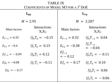
TABLE IX

COEFFICIENTS OF MODEL M3 FOR A 32 _DOE

𝐋𝟖𝟓 𝐋𝟕𝟎

𝑀 = 2.95 𝑀 = 3.287

Main factors Interactions

XJXT

Main factors Interactions XJXT 𝐸𝑇−1= 0.35 𝐼𝐽0𝑇0= −0.15 𝐸𝑇−1= 0.32 𝐼𝐽0𝑇−1= 0.04 𝐸𝑇1= −0.4 𝐼𝐽1𝑇0= 0.15 𝐸𝑇1= −0.38 𝐼𝐽_{= −0.04} 1𝑇−1 𝐸𝐽−1= − 0.09 𝐼𝐽0𝑇1= 0.12 𝐸𝐽−1 = − 0.12 𝐼𝐽0𝑇0= − 0.11 𝐸𝐽0= −0.08 𝐼𝐽1𝑇1= −0.11 𝐸𝐽1= − 0.17 𝐼𝐽1𝑇0= 0.10 𝐸𝐽₁= − 0.17 𝐼𝐽0𝑇1= 0.06 𝐼𝐽1𝑇1= − 0.06

It can be seen in Table IX, that the effects of XJ and XT are

not the same if the interval [-1; 1] is decomposed into two intervals [-1; 0] and [0; 1], Moreover, it can be noticed that the effects of the interactions (specially the interaction with the level 0) are significant. Nevertheless, the effects do not vary a lot from the 𝐿85 model to the 𝐿70 one. However, the

effect of the current, at level -1 increase mostly with aging which can indicate a snowballing effect of the current density with time.

D. Model of the second order with interactions based on Surface Response (model M4)

The factorial plan with 3 equidistant levels (-1, 0 and 1) can be the basis of a new DoE including quadratic effects on each of the factors, in order to introduce some non-linear effects. The model is given by (7) according to the Surface Response method [28]. Experiments 1 to 9 of Table V were used to estimate is coefficients:

𝑀4 = 𝐿𝑜𝑔(𝐿𝑥) = 𝑀 + 𝐸𝐽𝑋𝐽+ 𝐸𝑇𝑋𝑇+ 𝐼𝐽𝐽𝑋𝐽2+ 𝐼𝑇𝑇𝑋𝑇2

+ 𝐼𝐽𝑇𝑋𝐽𝑋𝑇

(7)

The quadratic effects of current density and temperature are

IJJ and ITT respectively. Table X lists all the coefficients

estimated by OLS.

TABLE X

ESTIMATED COEFFICIENTS FOR MODEL M4 𝐋𝟕𝟎 𝐋𝟖𝟓 M 3.396 3.083 EJ -0.148 -0.131 ET -0.348 -0.375 IJJ -0.079 -0.122 ITT -0.084 -0.075 IJT -0.007 -0.009

Temperature appears as the most influential parameter with the strongest effect when compared to that of current density. A large quadratic effect of both factors is also put in evidence and the values of IJT estimated by models M1 and

M4 are the same.

E. Discussion

Fig.12 shows a comparison between the lifespan models M1 to M4 for both luminances L70 and L85 where it can be

seen that most of the errors remain under 25%.

These models can be classified with respect to their accuracy, from the least to the most: M2.x<M1<M3<M4. The global conclusion is that non-linear models are more accurate than linear models. Indeed, M2.x type models, all the four models created from specific parts of the experimental plan are the less accurate for lifespan estimation even if their maximum error remains anyway under 30%. M1 model leads to maximum errors up to 12%. This is certainly due to the non-linear relationship between lifespan and the two stress factors, temperature and current density. The model M4 tends to be the best model therein, proving that the lifetime model is not of the first order p. The model M3 has zero percentage errors, which is normal because all the experiments are used in the learning set and there is no test set. Therefore, the errors cannot be comparable, despite having the ability to cope with a nonlinear phenomenon. Future work will test this model with additional test points.

Another possible conclusion is that, the errors between the

L85 and L70 lifespans differ, despite having a similarity. It can

be assessed that the differences in the lifespans show that the degradation of the OLEDs is a time varying process, even when the constant stress levels.

Fig. 12. Maximum percentage of error on lifespan modeling with the 7 models M1, M2.1 to M2.4, M3 and M4

The proposed method was able to provide good lifespan predictions. This confirms the accuracy of the forms used to model the link between the lifespan and the temperature and current density. The results show a high dependency between the lifespan and the operation

temperature, as already spotted in [30]. The model is build using experimental data with the assumption of the relation form between the lifespan and the stressors only. However, this might be a limitation for the proposed methodology if these relations are unknown.

VI. CONCLUSION AND PERSPECTIVES

Thanks to DoE, this work enriches the previous studies on OLED lifespan modeling. The method proves to be very helpful for this purpose. Several models have been proposed and compared allowing the study of the relative importance of stress factors. Temperature has the strongest effect compared with that of current density and their possible interactions. The proposed models show good rather performance for lifespan prediction in most of the tested cases and non-linear models appear as the most accurate.

Future work will test a larger number of OLEDs for each experiment making possible a deeper analysis of the predictive quality of the models. The variability and statistical significance of models will be studied. Additional test points randomly configured would also allow the analysis of the dispersion and distribution of the lifespan and thus refine the choice of the model. Other parameters than luminance such as color rending index or equivalent electrical model parameters could be tested according to the proposed protocol. Finally, considering a time varying model can unite the values of the effects without the need of testing different lifespan levels.

ACKNOWLEDGEMENTS

Authors would like to warmly thank Dr Alaa Alchaddoud from Laplace Laboratory, LM team, for his precious help and expertise during the experimental tests carried out in this study as well as for the time he dedicated to perform them.

Work on Organic Light Emitting Diodes in LAPLACE laboratory has been partially supported by FEDER European and Occitania Region grants.

REFERENCES

[1] R. Bayerer, T. Herrmann, T. Licht, J. Lutz, M. Feller, “Model for power cycling lifetime of IGBT modules - various factors influencing lifetime”, in Proc. 2008, 5th International Conference on Integrated

Power Systems (CIPS), p. 1-6

[2] M. Ecker, J. B. Gerschler, J. Vogel, S. Käbitz, F. Hust, P. Dechent, D. U. Sauer, “Development of a lifetime prediction model for lithium-ion batteries based on extended accelerated aging test data”, Journal of

Power Sources, vol. 215, p. 248-257, 2012

[3] H. Huang, p. A. Mawby, “A lifetime estimation technique for voltage source inverters”, IEEE Transactions on Power Electronics, vol. 28, no 8, p. 4113-4119, 2013

[4] H. Wang, P. Diaz Reigosa, and F. Blaabjerg, “A humidity-dependent lifetime derating factor for DC film capacitors”, in Proc. 2015 IEEE

Energy Conversion Congress and Exposition (ECCE), p. 3064-3068

[5] S. C. Xia, R. C. Kwong, V. I. Adamovich, M. S. Weaver and J. J. Brown, "OLED device operational lifetime: insights and challenges," in Proc. 45th Annual 2007 IEEE International Reliability Physics

Symposium, pp. 253-257

[6] X. Zhou, J. He, L. S. Liao, M. Lu, M. X. Ding, Y. X Hou, M. X. Zhang, Q. X. He and T. S. Lee, "Real-time observation of temperature rise and thermal breakdown processes in organic LEDs using an IR imaging and analysis system," Advanced Materials, vol. 12, no. 4, pp. 265-269, 2000

[7] J. Kundrata and A. Barić, "Electrical and thermal analysis of an OLED module", in Proc. Comsol Conference, Europe, 2012

[8] B. Geffroy, P. Le Roy and C. Prat, "Organic light emitting diode (OLED) technology: materials, devices and display technologies"

Polymer international, vol. 55, no. 6, pp. 572-582, 2006

[9] Y. S. Tyan, "Organic light-emitting-diode lighting overview," Journal

of Photonics for Energy, vol. 1, no. 1, pp. 011009-011009-15, 2011

[10] J. I. Park and S. J. Bae, "Direct prediction methods on lifetime distribution of organic light-emitting diodes from accelerated degradation tests", in IEEE Transactions on Reliability, vol. 59, no. 1, pp. 74-90, 2010

[11] Y. Zhu, N. Narendran, J. Tan and X. Mou, "An imaging-based photometric and colorimetric measurement method for characterizing OLED panels for lighting applications," in Proc. 2014 SPIE

International Society for Optics and Photonics Thirteenth International Conference on Solid State Lighting

[12] UL 8752: Organic Light Emitting Diode (OLED) Panels, 2013 [13] IEC 62868: Organic light emitting diode (OLED) panels for general

lighting - Safety requirements, 2014

[14] T. Tsujimura, K. Furukawa, H. Ii, H. Kashiwagi, M. Miyoshi, S. Mano, H. Araki and A. Ezaki, "World’s first all phosphorescent OLED product for lighting application" in Proc. IDW 2011 Digest, pp. 455

[15] K. Kwak, K. Cho and S. Kim, "Analysis of thermal degradation of organic light-emitting diodes with infrared imaging and impedance spectroscopy" in Optics express, vol. 21, no. 24, pp. 29558-29566, 2013

[16] A. Cester, D. Bari, J. Framarin, N. Wrachien G. Meneghesso, S. Xia, V. Adamovich and J. J. Brown, "Thermal and electrical stress effects of electrical and optical characteristics of Alq3/NPD OLED"

Microelectronics Reliability, vol. 50, no. 9, pp. 1866-1870, 2010

[17] H. Pang, L. Michalski, M. S. Weaver, R. Ma and J. J. Brown, "Thermal behavior and indirect life test of large-area OLED lighting panels," Journal of Solid State Lighting, vol. 1, no. 1, pp. 1-13, 2014 [18] J. Zhang, T. Zhou, H. Wu, Y. Liu, W. Wu and J. Ren,

"Constant-step-stress accelerated life test of white OLED under Weibull distribution case”, IEEE Transactions on Electron Devices, vol. 59, no. 3, pp. 715-720, 2012

[19] J. Zhang, F. Liu, Y. Liu, H. Wu, W. Wu and A. Zhou, "A study of accelerated life test of white OLED based on maximum likelihood estimation using lognormal distribution", IEEE Transactions on

Electron Devices, vol. 59, no 12, pp. 3401-3404, 2012

[20] J. Zhang, W. Li, G. Cheng, X. Chen, H. Wu, M. H. Herman Shen, "Life prediction of OLED for constant-stress accelerated degradation tests using luminance decaying model", J. Luminesc., vol. 154, pp. 491-495, 2014.

[21] H. Kim, H. Shin, J. Park, Y. Choi and J. Park, "Statistical modeling and reliability prediction for transient luminance degradation of flexible OLEDs," 2018 IEEE International Reliability Physics Symposium (IRPS), Burlingame, CA, 2018.

[22] D. W. Kim, H. Oh, B. D. Youn and D. Kwon, "Bivariate Lifetime Model for Organic Light-Emitting Diodes," in IEEE Transactions on Industrial Electronics, vol. 64, no. 3, pp. 2325-2334, 2017.

[23] F. Salameh, A. Picot, M. Chabert, P. Maussion, "Parametric and non-parametric models for lifespan modeling of insulation systems in electrical machines", IEEE Transactions on Industry Applications,

Special Issue on Fault Diagnosis of Electric Machines, Power Electronics and Drives, vol. 53, no. 3, pp. 3119-3128, 2017

[24] M. Szczepanski, D. Malec, P. Maussion, B. Petitgas and P. Manfé, "Prediction of the lifespan of enameled wires used in low voltage inverter-fed motors by using the Design of Experiments (DoE)"in

Proc. IEEE Industry Applications Society Annual Meeting, 2017

[25] A. Alchaddoud, L. Canale, G. Ibrahem and G. Zissis, "Photometric and electrical characterizations of large area OLEDs aged under thermal and electrical stresses," IEEE Transactions on Industry

[26] R. Fisher, The design of experiments, Oliver and Boyd, 1935

[27] G. Taguchi and S. Konishi, Orthogonal arrays and linear graph, American Supplier Institute Press, Michigan, 1987

[28] A. I. Khuri and S. Mukhopadhyay, “Response surface methodology”, Wiley Interdisciplinary Reviews: Computational Statistics, vol. 2, no. 2, pp. 128-149, 2010

[29] F. Salameh, A. Picot, L. Canale, G. Zissis, P. Maussion, and M. Chabert, “Parametric lifespan models for OLEDs using Design of Experiments (DoE)”, IAS’2018, Industrial Application Society Annual Meeting, Portland, OR, USA.

[30] A. Gassmann, S.V. Yampolskii, A. Klein, K. Albe, N. Vilbrandt, O. Pekkola, Y.A. Genenko, M. Rehahn, H. von Seggern, “Study of electrical fatigue by defect engineering in organic light-emitting diodes”, Mater. Sci. Eng. B 192, pp. 26-51, 2015.

AUTHORS

Farah Salameh, PhD. Born in Beirut in

1990, she got the Electrical Engineering degree from the Lebanese University in 2013. She got her M.Sc. in the Advanced control of Electric Systems in 2013 from Institut National Polytechnique de Toulouse (INPT), Toulouse, France and her Ph.D. in the Diagnosis and Prognosis of Electric Systems in 2016 from INPT. Her main research interest is the control and the diagnosis of electric systems and particularly the lifespan modeling of electrical engineering components. She is currently a part-time instructor at the Lebanese International University (School of Engineering - Electrical and Electronic Engineering department).

Andrea AL HADDAD, PhD Student. Born in Lebanon in

1995, has graduated in 2018 from engineering faculty of Lebanese University in electrical engineering. She got her MSc in Electrical Engineering Systems in 2018 from National Polytechnic Institute of Toulouse (France). Currently, she is a PhD student at the laboratory of Plasma and Energy Conversion (LAPLACE). Her main research includes the development of statistical methods for modelling and validating the degradation of electrical engineering components.

Antoine PICOT, PhD, graduated from

the Telecom Department of the Institut National Polytechnique (INP) Grenoble, France in 2006. He received the MS. degree in signal, image, speech processing and telecommunications in 2006 and his PhD. in automatic control and signal processing in 2009 from the INP Grenoble. In 2010, he was a post-doctoral fellow at the University of Chicago. Since 2011, he is an associate professor at the INP Toulouse. He is also a Researcher with the Laboratory of Plasma and Energy Conversion

(LAPLACE). His research interests are in monitoring and diagnosis of complex systems using signal processing, statistics and artificial intelligence techniques.

Marie CHABERT (M’10), PhD, received

the Engineering degree in electronics and signal processing from ENSEEIHT, Toulouse, France, in 1994, and the M.Sc. and Ph.D. degrees in signal processing and the “Habilitation à Diriger les

Recherches” from the National Polytechnic Institute of Toulouse, Toulouse, in 1994, 1997, and 2007, respectively. She is currently a Professor of signal and image processing with INPT-ENSEEIHT, University of Toulouse, Toulouse. She is conducting research with the Signal and Communication Team, Institut de Recherche en Informatique of Toulouse.

Her research interests include nonuniform sampling, time– frequency diagnosis and condition monitoring, and statistical modeling of heterogeneous data in remote sensing.

Laurent CANALE, PhD, MIEEE’12, SMIEEE’19, CNRS Research Engineer in

LAPLACE Laboratory in Toulouse (France). Born in Saint-Martin d'Hères (France) in 1972, and holds a Master and PhD focusing on High Frequencies Electronics and Optoelectronics from Limoges University, France, in 1998 and 2002. He published about magnetic thin films but his main PhD work was in pulsed laser deposition of lithium niobate thin films for optical telecommunications. From 2004 to 2010 he worked as Research Engineer for the National Research Institute of Agronomy in Bioemco Lab. (Paris, France). In 2010, he joined the National Center for Scientific Research (CNRS) and work in LAPLACE Lab., "Light & Matter" Team where his research focused on powerless light sources as LED and OLED with special interest in aging mechanisms. Since 2014, he is the Regional President of the French Illuminating Engineering Society (AFE). He is elected member of the research commission and the academic council of Toulouse 3 University since 2018 and, since 2019, he is the Secretary of Industrial Light and Display Committee of the Industrial Application Society of IEEE (ILDC).

Georges ZISSIS, PhD, MIEEE’92, SMIEEE’06. Born in

Athens in 1964, has graduated in 1986 from Physics department of University of Crete in general physics. He got his MSc and PhD in Plasma Science in 1987 and 1990 from Toulouse 3 University (France). He is today full Professor in Toulouse 3 University (France). His primary area of work is in the field of Light Sources Science and Technology. He is especially interested in the physics of electrical discharges used as light sources; system and metrology issues for

solid-state lighting systems; normalization and quality issues for light sources; impact of lighting to energy, environment, quality of life, health and security; interaction between light source and associated power supply; illumination and lighting. He is director of “Light & Matter” research group of LAPLACE that enrols 20 researchers. He won in December 2006 the 1st Award of the International Electrotechnical Committee (IEC) Centenary Challenge for his work on normalization for urban lighting systems (in conjunction with IEEE, IET and the Observer). In 2009, he won the Energy Globe Award for France and he got the Fresnel Medal from the French Illuminating Engineering Society. In 2011 has been named Professor Honoris Causa at Saint Petersburg State University (Russian Federation) and he is President IEEE Industrial Application Society for the period 2019-20.

Pascal MAUSSION, PhD, MIEEE’06, SIEEE’17, got his PhD in Electrical

Engineering in 1990 from Université de Toulouse, Institut National Polytechnique (INP), France. He is currently full Professor at Université de Toulouse and researcher with CNRS research Laboratory: LAPLACE, LAboratory for PLAsma and Conversion of Energy in CODIASE (Control and Diagnostic of Electrical Systems) group. His research activities deal with the design of experiments as an optimisation and modelling tool in control and diagnosis, the diagnosis of electrical systems such as drives and lighting, the control of power converters for induction heating or energy efficiency improvement in renewable energy systems, life cycle assessment in renewable energy systems. He is currently Toulouse INP Vice President for the International Affairs.