Investigating added value of regional climate modeling in North
American winter storm track simulations
E. D. Poan1 · P. Gachon2 · R. Laprise1 · R. Aider3 · G. Dueymes1
Received: 5 August 2016 / Accepted: 2 May 2017
© The Author(s) 2017. This article is an open access publication
overestimated. When the CRCM5 is driven by ERAI, no significant skill deterioration arises and, more importantly, all storm characteristics near areas with marked relief and over regions with large water masses are significantly improved with respect to ERAI. Conversely, in GCM-driven simulations, the added value contributed by CRCM5 is less prominent and systematic, except over western NA areas with high topography and over the Western Atlantic coastlines where the most frequent and intense ECs are located. Despite this significant added-value on seasonal-mean characteristics, a caveat is raised on the RCM ability to handle storm temporal ‘seriality’, as a measure of their temporal variability at a given location. In fact, the driving models induce some significant footprints on the RCM skill to reproduce the intra-seasonal pattern of storm activity. Keywords Regional climate model · Added value · Storm tracking · Temporal seriality
1 Introduction
Extratropical Cyclones (ECs) account for a large fraction of mid-latitude rainfall as well as extreme and severe weather events such as heavy precipitation, snow storms, coastal waves and flooding, which are responsible for important socio-economic and human damage (e.g. Liberato 2014). Pfahl and Wernli (2012) have shown that, over the east-ern half of Northeast-ern America, more than 60% of the daily extreme precipitation (i.e. daily events with intensity above the 99th percentile) are coincident with ECs, and this num-ber increases northeastward, reaching 80% over the Cana-dian Maritimes.
EC dynamics is primarily explained by the presence of large-scale baroclinic energy due to strong horizontal Abstract Extratropical Cyclone (EC) characteristics
depend on a combination of large-scale factors and regional processes. However, the latter are considered to be poorly represented in global climate models (GCMs), partly because their resolution is too coarse. This paper describes a framework using possibilities given by regional climate models (RCMs) to gain insight into storm activity dur-ing winter over North America (NA). Recent past climate period (1981–2005) is considered to assess EC activity over NA using the NCEP regional reanalysis (NARR) as a reference, along with the European reanalysis ERA-Interim (ERAI) and two CMIP5 GCMs used to drive the Cana-dian Regional Climate Model—version 5 (CRCM5) and the corresponding regional-scale simulations. While ERAI and GCM simulations show basic agreement with NARR in terms of climatological storm track patterns, detailed bias analyses show that, on the one hand, ERAI presents statistically significant positive biases in terms of EC gen-esis and therefore occurrence while capturing their inten-sity fairly well. On the other hand, GCMs present large negative intensity biases in the overall NA domain and par-ticularly over NA eastern coast. In addition, storm occur-rence over the northwestern topographic regions is highly
* E. D. Poan
emmanuel.poan@gmail.com
1 Dép. des Sciences de la Terre et de l’atmosphère, Centre
Pour l’Étude et la Simulation du Climat à l’Échelle Régionale (ESCER), Université du Québec à Montréal (UQAM), PO Box 8888, Stn. Downtown, Montréal, Québec H3C 3P8, Canada
2 Dép. de Géographie, ESCER Research Centre, University
of Québec at Montréal, Québec, Canada
3 Recherche en Prévision Numérique, Environment
temperature gradients between polar and tropical air masses in mid-latitudes (e.g. Sanders and Gyakum 1980; Chang et al. 2002). Other regional/small scale processes that merit consideration are lee cyclogenesis (cyclone development on the leeward side of topography) and coastal cyclogene-sis (in the presence of a large land-sea temperature contrast, such as between the cold North American continent and the warm waters of the Gulf Stream). Among others, Stull (2000) has stressed the importance of moisture availability, while Gachon et al. (2003) have highlighted the importance of the local temperature Laplacian and sensible heat fluxes (e.g. along the sea-ice margin in winter months) in increas-ing vorticity and therefore storm growth rate.
Representing these features in models is challenging from both weather and climate perspectives. For instance, Colle et al. (2015) have reviewed historical and future changes of EC activity along the East Coast of the USA and have pointed out that global climate models (GCMs) have difficulty in capturing the role of certain key features such as sea surface temperature (SST) gradients, latent heat release within storms, and also dynamical interactions with the jet stream. However, recent studies using GCMs from the 5th phase of the Coupled Model Inter-comparison Project (CMIP5) have shown quite reasonable climatology in storm track patterns with respect to reanalysis products (e.g. Seiler and Zwiers 2016; Ulbrich et al. 2008). In gen-eral, the comparison between GCMs and reanalyses has often shown negative bias for the intensity of ECs (e.g., Zappa et al. 2013), considerable dispersion when assessing intense to extreme storm events (Lambert and Fyfe 2006; Seiler and Zwiers 2016), and weaker cyclogenesis (Bengts-son et al. 2006; Pinto et al. 2006).
The coarse horizontal resolution of most GCMs pro-viding century-long climate simulations may present an important limitation for simulating realistic EC occur-rences and intensities. For instance, Jung et al. (2006) have shown that, at spectral truncation of T95, only 60% of observed storms are detected, while Colle et al. (2013) found that 6 of the 7 CMIP5 GCMs with resolution finer than 1.5° were able to better capture storm track maxima just north of the Gulf Stream, and to the east of southern Greenland. The resolution effect has also been invoked for weather reanalysis storm tracking. For instance, Trigo (2006) and Allen et al. (2010) have shown marked discrep-ancies in the number of storms detected when using the NCEP/NCAR (National Centers for Environmental Predic-tion/National Center for Atmospheric Research) reanalysis at 2.5° versus the ECMWF (European Centre for Medium range Weather Forecasts) 40-year one at 1.125° of horizon-tal resolution. On the other hand, Hodges et al. (2011) have shown smaller but still significant differences over North America (NA) between relatively fine resolution reanaly-ses, such as the ECMWF ERA-Interim reanalysis at 0.75°
and the NCEP CFSR (Climate Forecast System Reanalysis) at 0.5°.
To improve our understanding of storm activity and interactions with regional/local features, the present study takes advantage of finer grid-mesh datasets (0.44° × 0.44° model of the Coordinated Regional Climate Downscaling Experiment CORDEX—Giorgi et al. 2009) over North American simulations. This allows the added value (AV) of dynamical downscaling to be assessed with regard to EC characteristics such as occurrence, intensity, cyclo-genesis and -lysis regions over NA and oceanic boundaries (e.g., Pacific and Atlantic coasts). The Canadian Regional Cli-mate Model (RCM)—version 5 (CRCM5) is used for this purpose. In addition, an objective storm-tracking algorithm described in Sinclair (1994, 1997) is used to identify storm tracks and retrieve their parameters. This algorithm is part of the recent international initiative to compare various tracking methods under the Intercomparison of mid latitude storm diagnostics (IMILAST; Neu et al. 2013) project.
Direct comparisons between global and dynamically downscaled data can lead to systematic biases. Côté et al. (2015) have shown that evaluating EC activity in RCM against global data presents multiple challenges, including the sensitivity of cyclogenesis and cyclolysis to boundary effects. Nevertheless, a few recent studies have used RCM to analyze storm activity over the Western Atlantic Coast of North America (WAC) and the North Atlantic (e.g. He et al. 2013; Marciano et al. 2015). Long et al. (2009) have shown that an earlier version of the Canadian Regional Cli-mate Model could improve the representation of intense cyclones with respect to its driving GCM. Among other interesting points, RCMs provide an improved descrip-tion of the surface topography which, in the case of North America, is a decisive element in storm develop-ment (Brayshaw et al. 2009). While RCMs are reasonably appealing, it should not be forgotten that these models are driven by coarser datasets and therefore might inherit some biases from their boundary conditions. In addition, RCMs carry their own structural biases (Šeparović et al. 2013) due to many approximations, including the parameteriza-tion and numerical schemes used. Despite these uncertain-ties, RCMs may provide GCMs with a useful and comple-mentary tool for climate studies (e.g., Laprise et al. 2003; Laprise 2008) and, in particular, can help improve our comprehension and representation of storm activity. This is partly confirmed by the recent study by Colle et al. (2015), which pointed out that only 5–10% of cyclone densities are unpredicted over the West Atlantic when the ensemble RCM runs from the NARCCAP (North American Regional Climate Change Assessment Program—Mearns et al. 2009) project are used.
Finally, EC temporal ‘seriality’, described in Mailier et al. (2006) as the rate at which storms transit through a
given location, is a crucial aspect that needs to be well rep-resented in climate models. Over the eastern Atlantic, tem-porally clustered activity (larger than average storm tran-sits at a specific location) is often considered as a potential source of socio economic damage. For example, between 26th and 28th December 1999, two successive intense storms named Lothar and Martin (Ulbrich et al. 2001; Wer-nli et al. 2002; Goyette et al. 2003) transited over Europe, leading to about 130 human deaths and 13 billion Euros of economic losses. Conversely, over the western Atlantic, because of the quasi-permanent and strong winter baro-clinic energy, regular (i.e. persistent) storminess can be as damaging as clustered storms. Pinto et al. (2013) recently addressed the question of ‘seriality’ with regard to the cur-rent and future climate in mid-latitudes. They found that storm occurrences tended to be a regular process rather than being clustered at the entrance of the North Atlantic storm track. On the other hand, the same study showed that GCM projections suggested a change toward more clus-tered patterns over the WAC, consistent with the overall northward migration of the baroclinic zone. Vitolo et al. (2009) have shown that storms tend to be more clustered when only intense storms are considered (i.e. the 90th percentile). This paper gives an opportunity to gain more insight into the issue of EC temporal seriality over the NA domain and from reanalysis, RCM and GCM perspectives. In particular, regional storminess regimes (regular–inter-mittent–highly active) will be analyzed.
The paper is organized as follows. Data and method-ology are described and discussed in Sect. 2. Section 3 assesses the climatology of storm characteristics in rea-nalyses and GCMs, and in CRCM5 simulations driven with different boundary conditions. Section 4 elaborates on the regional structure of storm temporal ‘seriality’ over known NA areas of active cyclogenesis. The main findings are summarized in Sect. 5, together with suggestions for fur-ther developments.
2 Data and methodology
2.1 Data: description of simulations 2.1.1 Reanalysis data
In the present study, two sets of reanalysis products are used:
1. NCEP North American Regional Reanalysis (NARR; Mesinger et al. 2006), available from 1979 to present, generated by a regional model nested in the NCEP-DOE (Department of Energy) global model. NARR is generated using the very high resolution NCEP Eta
Model (32-km with 45 vertical levels) together with the Regional Data Assimilation System that, signifi-cantly, assimilates precipitation along with the other atmospheric variables. Due to improvements in the model/assimilation system, NARR temperature, winds and precipitation are substantially better than those given by NCEP-DOE. Because of its finer resolution (0.25° × 0.25°; 3 hourly), which is more relevant for regional (scale) studies, NARR will be considered as the reference dataset in our analysis.
2. The ECMWF reanalysis ERA-Interim (hereafter ERAI; Dee et al. 2011), available from 1979 to the present, is a global reanalysis computed with the spec-tral horizontal resolution T255 (~80 km) and with 60 levels in the vertical. Data are archived on a 6 hourly basis. ERAI has been used by many studies to assess models (CMIP5) as well as in comparisons with other reanalysis datasets (e.g., Colle et al. 2013). Coté et al. (2015) have noted, however, that its relatively smooth topography over the Rockies can lead to overestimated cyclonic activity over western North America.
2.1.2 GCM and RCM simulations
Two GCMs taking part in the CMIP5 project and used for IPCC assessment reports (e.g., IPCC 2013) were used to provide boundary conditions for the RCM runs:
1. The Canadian Earth System Model, version 2— CanESM2 (Arora et al. 2011) is a global climate model developed by the Canadian Centre for Climate Modelling and Analysis (CCCma) of Environment and Climate Change Canada. The CanESM2 atmos-pheric component—CanAM4 (Canadian Atmosatmos-pheric Model 4, von Salzen et al. 2013) is a spectral model employing T63 triangular truncation with physical ten-dencies calculated on a ∼2.81° linear transform grid. CanESM2 historical natural and anthropogenic forcing simulations (1951–2005) are considered here to use direct atmospheric fields for the storm tracking analysis and also to drive the RCM model for both the atmos-pheric and oceanic boundary conditions.
2. The Max Planck Institute Earth System Model—MPI-ESM-LR (Giorgetta et al. 2013) is a global atmosphere, ocean and land surface coupled model. For the atmos-phere section, the low-resolution version is available at T63/1.9° and will be used over the historical period 1951–2005.
Finally, the Canadian Regional Climate Model version 5—CRCM5 is used to simulate atmospheric regional con-ditions following the protocol defined by the CORDEX
project. CRCM5 combines parts of the physics package of the Environment Canada Global Environmental Multi-scale (GEM) forecast model (Côté et al. 1998a, b) version 3 (GEM3), but uses the Canadian land-surface scheme CLASS 3.5 (Verseghy 2008) and the interactive coupled model “Flake” to account for lakes (Martynov et al. 2010). ERAI, CanESM2 and MPI-ESM-LR are used to provide three different (atmospheric and oceanic) boundary con-ditions to run the CRCM5 model using a 0.44° horizontal grid mesh on a rotated pole grid (see descriptions in Mar-tynov et al. 2013; Šeparović et al. 2013). CRCM5 data are provided on a 3 hourly basis. Finally, it is worth mentioning that no spectral nudging has been applied when conducting the CRCM5 dynamical downscaling experiments.
Table 1 gives details of all the datasets used in this study. Before the storm-tracking algorithm (described in the next section) was run, simulations were all interpo-lated on a common 100-km polar stereographic (PS100) projection with an identical spatial extent. This was done for both global- and regional-scale simulations extracted over the regional domain of interest (see Fig. 1). As shown by Eichler and Gottschalck (2013), storm tracking is sen-sitive to the dataset spatial resolution and re-gridding the simulations to a “GCM-RCM intermediate resolution” (i.e. 100 km) is believed to help reduce this sensitivity. Because our focus is on synoptic-scale ECs, this intermediate res-olution should be able to capture all major winter events regardless of the original resolution. Finally, even though differences in time resolution can play a significant role in EC characteristics (see Blender and Schubert 2000), simu-lations will be kept at their initial resolutions (i.e. 3 hourly for regional products as NARR and CRCM5, and 6 hourly
for the rest, i.e. available archived fields common to all global reanalysis and GCMs).
2.1.3 Oceanic boundary conditions
To diagnose the ocean related baroclinic energy (e.g., Branscome et al. 1989) provided by the boundary condi-tions (reanalysis and GCMs), SSTs are evaluated. Seiler
Table 1 Data sets used for the storm tracking
See text for details about climatological time period and native resolutions
Simulation function Simulation type Simulation short name Native time/ space resolu-tion
Time period/domain Long name/Institution Reference Regional Reanalysis NARR 0.25°/3 hourly 1979–2012/ North
America (NA) NCEP North American Regional Reanalysis (USA) Driving data Global Reanalysis ERAI 0.75°/6 hourly 1961–2012/Global European Centre for Medium
range Weather Forecast Reanalysis (EU) GCMs CanESM2 1.875°/6 hourly 1961–2005/ NA Canadian Earth System
Model—Environment and Climate Chance Canada (ECCC- CANADA) MPI-ESM-LR 1.875°/6 hourly 1961–2005/ NA Max Planck Institute Earth
System Model (GERMANY) Regional climate model RCM CRCM5 0.44°/3 hourly 1961–2012/NA Canadian Regional Climate
Model - Université du Québec à Montréal (UQAM- CANADA)
Fig. 1 NARR North America surface topography at 0.25° over the
domain used to track the ECs. The solid black line contours elevation above 500 m. Regions of interest for the study are delimited by the 4 boxes: ALB Alberta, COL Colorado, GL Great Lakes, WAC Western Atlantic Coast
and Zwiers (2016) have shown that GCM skill is strongly impacted by SSTs and the related upper tropospheric jets. For NARR, over open water (seas and lakes), SSTs are derived from 1° SST observations by Reynolds et al. (2002) while, when sea/lake ice is detected (e.g. frozen lakes or sea), SSTs stand for the surface skin temperature derived from the energy balance equation (see Mesinger et al. 2006). For ERAI, the prescribed boundary condi-tions are taken from different sources (Kumar et al. 2013) as follows: from January 1989 to June 2001, NCEP 2D-Var SSTs; from July 2001 to December 2001 NOAA (National Oceanic and Atmospheric Administration) Optimum Inter-polation SSTs; from January 2002 to January 2009, NCEP Real-Time Global SSTs; and from February 2009 onwards, the Met Office Operational SSTs and Sea-Ice Analysis (OSTIA). As in NARR, the open ocean SSTs are derived from these observations. However, in the presence of sea ice, ERAI SSTs are assumed to be −1.7 °C, corresponding to the average temperature of frozen seawater (at a salinity of 34‰). The 2 GCMs use SSTs from their oceanic mode-ling component where frozen SST is set constant and close to −1.7 °C. Since the analysis is done during the winter, the northern Canadian seas/lakes are mostly frozen and large differences are expected from NARR and the other three datasets. Therefore, comments related to SST structure are limited to open water areas.
2.2 Methodology
2.2.1 Storm tracking algorithm: detection criteria and tracking approach
A modified version of Sinclair’s (1994, 1997) storm-track-ing algorithm was used to retrieve individual cyclone tra-jectories for all simulations described in Table 1. Actually, Sinclair (1997) used the 1000-hPa geopotential heights to compute the vorticity field. However, the NA topographic features (higher than 1000 m over the western half of the region in Fig. 1) make it hard and rather inconvenient to use this level, particularly over the western side. Also, GCM fields are not systematically archived at 1000 hPa, especially the geopotential height or wind fields. For a more convenient and consistent evaluation of ECs over NA, atmospheric variables at 850-hPa will be used. The tracking algorithm has also benefitted from several years of develop-ment at UQAM (University of Quebec At Montréal; e.g., Rosu 2005; Radojevic 2006), but only the main steps (orig-inally from Sinclair’s previous work) are reviewed here: 1. 850 hPa winds are spatially derived to obtain the
rela-tive vorticity (𝛇r) and this latter variable is spatially
smoothed to remove smaller scale features or addi-tional biases due to original grid resolution that is
significantly different between GCMs and RCMs. To do so, a Cressman’s filter is used to average data at each grid point with neighboring grid points within a 800 km radius circle.
2. 𝛇rlocal maxima exceeding the 1.5 CVU (cyclonic
vor-ticity unit, 10− 5 s− 1) are taken as cyclonic centers (CC)
for the tracking process. A bicubic spline fit is used in order to locate the CC more accurately.
3. Many detected CC are stationary orographic features resulting from lee troughs or heat lows. These spurious centers are eliminated by requiring centers to have a total displacement of at least 1200 km in 24 h, equiva-lent to a horizontal speed of about 50 km h− 1 (often
observed for winter synoptic scale disturbances over NA; Arhens 2009)
4. EC life cycle construction is based on probabilistic functions involving the previous/current/next positions of the CC and the 500-hPa wind modulus. It is com-monly accepted as a ‘forecaster rule’ in meteorology that storms move approximately along the 500-hPa wind and the speed at which surface systems travel is estimated as half the 500-hPa wind speed (e.g., Ahrens 2009). A match is attempted between each of these pre-dictions (location) and the set of nearest centers found a time step later. An ensemble of successfully chosen matches satisfies the condition of minimizing a cost function, which is a weighted sum of absolute depar-tures of position, pressure and vorticity from predicted values (Murray and Simmonds 1991; Sinclair 1994). 5. The variables retrieved from the tracking are
repre-sentative of a reference surface of 2.5° × 2.5° (defined as 1 SU, surface unit) and are defined as follows: (1) Cyclone occurrence, also often referred to as frequency or track density, which is the number of 3-hourly (or 6-hourly) CC detected and associated with a track (unit = #CC SU− 1 month− 1); (2) Cyclone intensity,
which is the relative vorticity (in CVU) associated with the CC, (3) Cyclone genesis and lysis rates (#CC SU− 1 month− 1), which simply refer to the first and last
points in the cyclone track respectively.
It is worth mentioning that, in the present study, “win-ter season” refers to the northern hemisphere cold sea-son extending from November to March and will be noted NDJFM. Model skill will be primarily compared with NARR but also with ERAI in order to link the cur-rent results with previous studies. Statistical significance tests will be performed in the sense of Mann–Whit-ney–Wilcoxon tests (Wilcoxon 1945) at the 99% signifi-cance level.
2.2.2 Winter storm temporal seriality
To study winter storm temporal ‘seriality’, an approach similar to that of Mailier et al. (2006) was used, as in the recent work over the North Atlantic by Pinto et al. (2013). If cyclone occurrences were completely random (i.e., the occurrence of one cyclone at any moment is independent of previous cyclone occurrences), its distri-bution could be described by a one-dimensional Poisson process with a constant rate or intensity (=seasonal mean at each location). Two alternative hypotheses to complete randomness are possible: (1) serial clustering, according to which the passage of one cyclone could trigger other cyclones as the energy propagates downstream, and (2) serial regularity, which may arise if favorable background conditions help to maintain a regular rate of cyclogenesis and the resulting cyclones are permitted to occur within a minimum time–space distance. To verify these hypoth-eses, the monthly occurrence (N) time series (at each grid point) are considered and a storm dispersion index φ is computed as follows (see Pinto et al. 2013):
where Var(N) stands for the monthly temporal variance and E(N) the monthly mean. A parameter defined in this way compares storm dispersion to a Poisson’s process with dis-persion 1. Following Eq. (1), the three previously defined hypotheses can be expected:
(1) 𝜑 =
Var(N) E(N) − 1
1. 𝜑 = 0, monthly counts are randomly distributed [Var(N) = E(N)], and therefore storm occurrences fol-low a homogeneous Poisson process.
2. 𝜑 > 0, the process is more dispersive than a simple Poisson process and so cyclone occurrences are tempo-rally clustered (i.e. intermittent process).
3. 𝜑 < 0, the process is under-dispersive and therefore cyclone transits at the given location tend to be a recur-rent or regular process.
3 Winter storm characteristics
3.1 Reanalysis and global climate model simulations 3.1.1 Winter cyclone genesis and lysis pattern
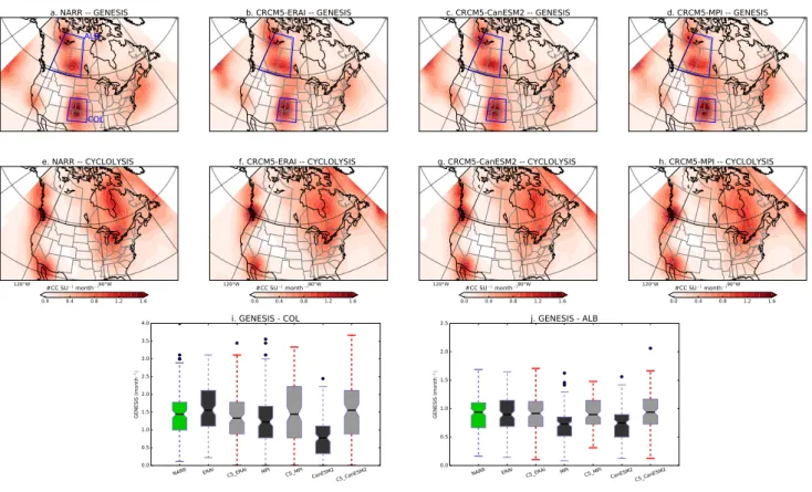
Figure 2 displays spatial structures of storm genesis (top) and lysis (bottom) rates as defined in the “ Methodol-ogy” section, for NARR and the three driving datasets. According to Neu et al. (2013), these two parameters are the most subject to discrepancy among methods and mod-els. The discussion focuses on the inner domain as cyclo-genesis over the Pacific and cyclolysis over the Atlantic are affected by the boundary locations of the regional simulated domain (close to inflow/outflow over the west-ern/eastern domain limits). Consistently with previous studies (e.g., Grise et al. 2013), both NARR and ERAI (Fig. 2a, b) reanalyses highlight two continental regions of cyclone initiation: the genesis of the so-called Alberta Clippers over western Canada (Stewart et al. 1995) and
Fig. 2 25-year (1981–2005) NDJFM climatology of storm genesis
(top panels) and lysis (bottom panels) rates in [#CC SU−1 month−1]
(i.e. cyclonic centers per surface unit SU; 1 SU = 2.5° × 2.5°) from: a NARR (used as reference), b ERAI, c CanESM2, and d MPI-ESM-LR. A threshold of 1.5 CVU (cyclonic vorticity units, 1
CVU = 10−5 s−1) is used for storm detection and tracking while a
min-imum of 24 h is required for the lifetime. The Alberta and Colorado regions delimited in a are highlighted for boxplot analysis shown in Fig. 6
the genesis of the Colorado Lows over the Midwest USA (Sisson and Gyakum 2004). While both reanalyses agree on a stronger genesis rate over Colorado, ERAI tends to overestimate cyclone initiation relative to NARR over this area. In addition to those in Colorado and Alberta, a secondary cyclogenesis region can be seen over the East Coast, with a local maximum near the New England Coast between Cape Hatteras and Cape Cod (well defined in NARR data and underestimated in the ERAI data). As shown by Grise et al. (2013), rather than being a cyclone initiation area, the East Coast region is more subject to a redevelopment or intensification of cyclones because of larger low level baroclinic gradients and also to the pres-ence of diabatic PV (potential vorticity) due to oceanic latent heat release (Lackmann 2011). Therefore, these coastal systems (also called “Nor’easters” by Hirsch et al. 2001) can be quite frequent and explosive (‘bombs’), reaching a growth rate that exceeds one bergeron (Seiler and Zwiers 2016) over the western boundary current (i.e. in the vicinity of the main Gulf Stream branch). The GCM realizations show rather poor skill compared to the reanalysis products: CanESM2 (Fig. 2c) strongly underestimates the number of cyclones that form in these three cyclogenesis regions, while MPI-ESM-LR (Fig. 2d)
reproduces more accurately the Colorado Lows genesis rate (as confirmed by the genesis boxplots in Fig. 6i).
The cyclolysis rate (bottom panels in Fig. 2e–h) indi-cates that the Rocky Mountains act as a strong barrier lead-ing to remarkable cyclolysis over their western limit (over British Columbia and California). There is also a remark-able lysis rate near the eastern sides of continental lakes or inland sea (Great Lakes or Hudson Bay) as the mean envi-ronment energy drops drastically after ECs cross from the moist, warm conditions over lakes or open waters to the dry, cold conditions over land. The cyclolysis rate is rather well captured by all four simulations in terms of spatial structures. However, and consistently with their weaker genesis rate, GCMs underestimate cyclolysis at the exit of the Great Lake region and over the eastern part of Hudson Bay, and do not capture the relatively large spatial variabil-ity displayed by reanalyses over eastern Canada.
3.1.2 Winter cyclone occurrence and intensity
Figures 3 and 4 present the NDJFM mean of storm occur-rence and intensity, respectively, over North America for NARR and the three driving datasets. Driving data biases relative to NARR (middle row) and ERAI (bottom) are
Fig. 3 Same as Fig. 2 but for storm occurrence (top panels). Driv-ing-data occurrence biases with respect to NARR (middle panels) and ERAI (bottom panels) are also shown. Statistically significant differences (biases) in the sense of a Mann–Whitney–Wilcoxon test
(Wilcoxon 1945) with p value <0.01 are shaded by black dots. [#CC SU−1 month−1] is the number of cyclonic centers per surface unit
also displayed. All datasets highlight the well-known storm-track pattern over North America marked by a white box over the Great Lakes region and the north Atlantic storm-track entrance over the WAC (Western Atlantic Coast) of the USA and Canadian Maritimes. Historical storm-track classification based on EC origin (Reitan 1974; Hoskins and Hodges 2002 among others) can also be inferred: (1) the West Coast Pacific storm-track termination over the western Rockies, (2) the lee-side tracks from both the Colorado and Canadian Alberta Rockies, merging over the Great Lakes area, and (3) the WAC track following the land–ocean boundaries and reaching an occurrence maximum near Nova Scotia and the eastern side of the Gulf of St. Lawrence. The Hudson Bay region is also marked by high occurrence of storms, well defined by the NARR data (Fig. 3a) and underesti-mated by the other products (Fig. 3b–d). In fact, Stewart et al. (1995) have shown that, during the winter season, both polar lows and synoptic storms transiting over the St. Lawrence Basin dissipate just after crossing the rela-tively warm water of Hudson Bay, some even regenerat-ing when open waters are sufficiently large in early winter (e.g., Gachon et al. 2003). On the other hand, a remark-able minimum (or absence) of cyclone occurrence can be seen over the Rocky Mountains, the southern border of
the Appalachian Mountains and, to a lesser extent, the Kaniapiskau Plateau in the North of Quebec.
Despite handling the main structures, the three driving datasets, including ERAI, exhibit notable differences with NARR (Fig. 3e–g). The ERAI biases, though surprisingly large, are reminiscent of those of Hodges et al. (2011), where ERAI was shown to overestimate storm occurrence, particularly over northern America, relative to two other reanalyses (NASA-MERRA and NCEP-CFSR) whose res-olution is close to that of NARR. It is worth recalling that ERAI occurrences compare well with those detected by Grise et al. (2013) using the same data, but with a differ-ent tracking algorithm. Overall, these biases raise the ques-tion of which data can be considered as references in model intercomparison exercises.
The 2 CMIP5 GCMs show, consistently with their lower (coarser) topography, a positive bias over the Canadian Rockies, i.e. they overestimate CC over regions with high relief (Fig. 3f, g). In contrast, the Hudson Bay maximum is underestimated. This is likely due to the lack of oceanic grid points, according to their coarse horizontal resolution, inducing an underestimation of regional-scale latent and sensible heat fluxes from open water areas present in early winter. Such fluxes are partly responsible for EC intensifi-cation or the development of polar lows (see Gachon et al. 2003). Over the East Coast, occurrence biases are moderate
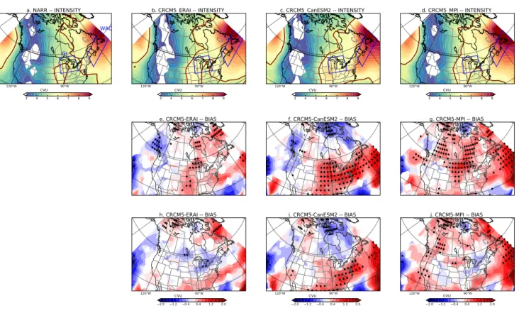
Fig. 4 Same as Fig. 3 but for storm intensity (in CVU). High intensity values (>5 CVU) are delimited with the dark brown contour. The Great Lakes and the Western Atlantic Coast regions are highlighted for occurrence and intensity boxplot analysis shown in Fig. 6
for both GCMs. However, when compared with ERAI, consistently with previous studies (e.g., Colle et al. 2013; Seiler and Zwiers 2016; Zappa et al. 2013), GCMs show a large negative occurrence bias near the East Coast and over the Gulf Stream area (Fig. 3c, d, f–i).
Despite differences in their occurrence field, the inten-sity of winter storms (Fig. 4) is relatively well captured by NARR and ERAI, showing large values (>5 CVU) east of the continental genesis region and reaching a maximum over the Newfoundland area. Bias assessment shows that ERAI slightly overestimates the intensity over the Great Lakes, where surface water temperature can play an impor-tant role before the formation of lake-ice. The GCM sim-ulations fail to capture the intensity amplitude. Red areas over the continental regions of NA imply that ECs of both GCMs are too intense with respect to NARR and ERAI. Over the East Coast, the negative bias pattern is very sali-ent (both in terms of location of maximum values and in spatial extent, especially for CanESM2 data). In fact, both GCMs follow the CMIP5 ensemble mean (e.g., Seiler and Zwiers 2016), being barely sensitive to the well-known WAC intense cyclones associated with the warm SSTs (the Gulf Stream water) or along the coast of eastern North America where land/sea temperature contrasts are high.
The SST anomalies shown in Fig. 5 are quite sub-stantial within these GCMs, particularly for CanESM2 and for the North Atlantic. Along the land/sea boundary, SST gradients constitute a good proxy when diagnosing the potentiality of storminess (Nakamura et al. 2004;
Hoskins and Valdes 1990). Boundary conditions brought by SST features (amplitudes, spatial and temporal vari-ability) can significantly impact the ability of a model to generate EC initiation, and then its development and/ or intensification for those arriving from continental regions. Woollings et al. (2010) have shown that SST spatial and temporal resolutions (considering that they correspond to prescribed values over open water areas in RCM), strongly influence the ability of an RCM (and a GCM) to capture the key features of storms. Colle et al. (2015) have concluded that the question of whether it is SST values or their gradients that influence storms most is still open. Similarly, Booth et al. (2012) have shown that storm strength increases monotonically with SST magnitudes, even for weak SST gradients, and have con-cluded that “the SST beneath the storm can have just as important a role as the SST gradients in local forcing of the storm”. With such warm biases of SSTs, GCMs would be expected to provide more humidity and thus diabatic heating (latent and sensible) PV, which, in turn, should increase storm development (Bluestein 1993). Instead, SST does not appear to be such a decisive com-ponent in determining GCM ability to simulate EC char-acteristics, i.e. at the scale of a GCM. Zappa et al. (2013) have consistently shown that prescribing “observed” SSTs as boundary conditions in CMIP5 GCMs does not significantly suppress this negative bias in intensity or EC occurrence over the WAC. Ultimately, the lack of fine spatial, and particularly temporal, resolution for SST
Fig. 5 25-year NDJFM mean SST (°C) from NARR (a) and the
3 driving (ERAI, CanESM2, and MPI-ESM-LR) datasets (b–d, respectively). The bottom panels represent climatological bias with respect to NARR from ERAI (e), CanESM2 (f) and MPI-ESM-LR (g), respectively. Over the open ocean, SSTs represent the sea surface
temperatures for all datasets while, over frozen areas, SST definition may vary. See text for more details. Gray shaded areas correspond to the presence of sea-ice in March (maximum extent during the November to March period) for each dataset
seems to be the key factor preventing improved climate model skill with respect to coastal EC characteristics. This was demonstrated, at least at the short-term syn-optic scale, over the Gulf of St. Lawrence area in early winter, where the high frequency (high resolution) cou-pling between atmosphere and ocean has quite a substan-tial impact on the accuracy of meteorological forecasts over the whole area, especially when ECs are involved (Gachon and Saucier 2003; Pellerin et al. 2004). In fact, the high resolution and frequency interactions between atmosphere and surface oceanic conditions from the fall to winter months can strongly modify SST and sea-ice conditions at the daily scale (e.g., Gachon et al. 2001), leading to substantial modification in the surface and the air temperature gradients (see Bourassa et al. (2013) for a related discussion on turbulent surface fluxes and air/ ocean and sea-ice interactions). All these surface forcing factors and potential SST biases play a key role in EC development and intensification at high resolution over oceanic areas, i.e. from the RCM simulations analyzed below.
3.2 Assessment of CRCM5 storm characteristics 3.2.1 Storm genesis and lysis
In the following, the analysis seeks to assess the regional model structural error occurring when the model is driven by the most accurate available boundary condi-tions (i.e. reanalysis ERAI products) and, secondly, the value added by regional modeling (Di Luca et al. 2015) with respect to global climate simulations (MPI-ESM-LR and CanESM2) also used as boundary conditions. Figure 6 displays winter storm genesis (Fig. 6a–d) and lysis (Fig. 6e–h) for NARR (for easier comparison) and the 3 simulations of CRCM5. In addition, genesis rate boxplots computed for the Colorado (Fig. 6i) and the Alberta (Fig. 6j) regions are displayed. It is worth recalling that the boxplots do not include spatial vari-ability since the genesis variable is spatially averaged, so statistics are computed over the monthly time series. ERAI-driven CRCM5 (Fig. 6b) captures the genesis pattern exhibited by NARR remarkably, outperforming ERAI over both continental initiation areas (Colorado
Fig. 6 Top (a–h) same as Fig. 2a, e but for CRCM5 simulations driven by ERAI (b, f), CanESM2 (c, g), and MPI-ESM-LR (d, h) respectively. Bottom (i, j) 25-year NDJFM monthly storm gene-sis boxplot for all simulations over the Colorado (i) and Alberta (j) regions (see NARR top panel for their respective locations). The reference NARR is in green, driving data are in black and the
cor-responding CRCM5 simulations are in gray with red whiskers. Box-plots show the min, max and the 3 quartiles (25th, 50th, 75th per-centile) and also the outliers (in blue) that fall out of the interval [Q1–1.5 × IQR, Q3–1.5 × IQR] where Q1 and Q3 are the first and third quartiles and IQR the Inter Quartile Range. Note that C5 (i, j) corresponds to CRCM5
and Alberta). Similarly, the CanESM2-driven simu-lation genesis (Fig. 6c) is improved over the continent and at the East Coast, as can be seen from the boxplots (Fig. 6i, j) where the median is shown to be very close to NARR one. A minor improvement is seen in MPI-ESM-LR-driven CRCM5 (Fig. 6d), with the rate of cyclogen-esis increasing towards the NARR rate over Alberta. It should be noted that, for both GCM-driven simulations, although significant improvement occurs for both mean (from ~0.6 to ~1 CC SU− 1 per month which is NARR
value) and dispersion parameters over the Alberta region, the Colorado boxplots suggest that only the gen-esis (NDJFM) mean value is well captured by CRCM5, while dispersion is much more than observed. To sum up, despite this appreciable AV over continental areas, it appears that there still is room for improvement over the East Coast where CRCM5 tends to reproduce (or mimic) the patterns of GCMs, resulting in underestimation or spatial shift of genesis in comparison with NARR. Finally, the cyclolysis rate shows consistency among all regional simulations. Over the eastern sides of the Great Lakes and Hudson Bay, CRCM5 increases the cyclone dissipation frequency, which was underestimated by both GCMs. The same improvement can be seen over the southern California coast.
3.2.2 Storm occurrence and intensity
Figures 7 and 8 present storm occurrence and intensity (respectively) simulated by CRCM5 driven with the three different boundary conditions, together with the associ-ated biases with respect to NARR and ERAI. In addition, to evaluate each variable distribution more accurately, box-plots of storm occurrence and intensity spatially averaged over the Great Lakes and the WAC are displayed in Fig. 9. Among the three versions of CRCM5, the ERAI-driven one clearly shows the lowest and mostly statistically non-signif-icant biases for both occurrence (Fig. 7b, e) and intensity (Fig. 8b, e) parameters and for the whole of NA excluding arctic regions. In fact, the ERAI positive occurrence bias (discussed in Fig. 3b) is reduced by about a factor two over the continent, along the East Coast and over the Atlantic by the ERAI-driven CRCM5. On the other hand, Fig. 8b suggests that, for the intensity parameter, both ERAI and CRCM5-ERAI biases are comparable (for instance over the Great Lakes) and are mostly not statistically significant.
GCM-driven simulations (Fig. 7c–f, h, i) display large and statistically significant occurrence biases, especially over the southeast of the USA and onto the Atlantic ocean when comparison is made with ERAI. Neverthe-less, when the RCM is considered with respect to its driving GCM, Fig. 9a (for WAC occurrence) shows a
Fig. 8 Same as Fig. 4 but for CRCM5 simulations driven by ERAI (b, e and h), CanESM2 (c, f and i) and MPI-ESM-LR (d, g and j)
Fig. 9 Same as Fig. 6i, j but for monthly storm occurrence and intensity over the Western Atlantic Coast (WAC, a and c) and the Great Lakes (GL, b and d)
slight improvement in terms of storm occurrence over the Western Atlantic coast, with, for instance, an inter-quartile range that is more compatible with NARR for the CRCM5 simulations. Conversely, over the Great Lakes (Fig. 9b), no clear difference appears with respect to GCM simulations.
Considering the EC mean intensity (Fig. 8), GCM negative bias is replaced by a positive bias along the majority of the East Coast in the CRCM5 runs (Figs. 8c, d, f, g, i, j, 9c), which is potentially due to the exacerbat-ing influences of positive biases (too warm) in the SSTs over the western Atlantic (Gulf Stream area) including over the Labrador Sea in the MPI runs, as suggested in Sect. 3.1.2. Finally, it appears that, near areas with marked relief, CRCM5 captures EC occurrence and intensity accurately and thus brings clearer AV than over the south east of North America and the North Atlantic.
4 Temporal seriality of North America ECs
This section analyzes the ‘seriality’ of storms based on their monthly count (occurrence) time series at model grid point scale. The dispersion parameter described in Sect. 2.2.2 is firstly assessed to diagnose CRCM5 (and driving model) skill in capturing some aspects of the intraseasonal (monthly) variability related to EC activ-ity. Furthermore, regional storm occurrence and inten-sity distributions are assessed in order to determine the NA storminess regimes.
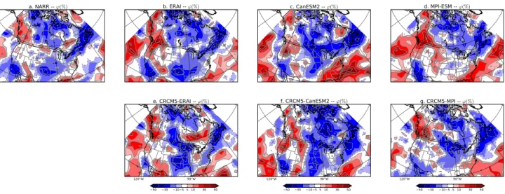
4.1 Storm dispersion maps
Figure 10 displays the dispersion parameter φ (in %) in the same manner as in Pinto et al. (2013). Over the northern regions (Western and Northern Hudson Bay, and Canadian Arctic), there is decent consistency among all datasets, showing that storm occurrence is under-dispersive (φ < 0). In other words, it is a recurrent and regular phenomenon and so its monthly variability is rather weak over these regions, in agreement with Serreze (1995) and Stewart et al. (1995), who diagnosed frequent cyclogenesis activity (due to polar lows and associated blizzards) over the (Cana-dian and Alaskan) Arctic throughout the winter season.
Over the continental US, NARR (Fig. 10a) displays a southwest-northeast axis of storm regularity, in agreement with Vitolo et al. (2009) and Mailier et al. (2006), suggest-ing persistent storminess throughout the winter season. Such a regime originates from the eastern flank of the Col-orado genesis region, passing successively across the Great Lakes, the St. Lawrence valley and the East Coast. This is also consistent with the quasi-permanent baroclinic energy generated by southern warm air masses (Gulf of Mexico and WAC) and the winter continental and/or polar cold air masses. On the other hand, close to the very continental cyclogenesis “points” (Alberta and Colorado as shown in Fig. 3a) and westward, storm occurrence is rather intermit-tent (clustered), partly reflecting the frequency at which upper tropospheric shortwave troughs cross and “emerge from” the Rocky Mountains. Despite significant differences in terms of seasonal mean occurrence, ERAI (Fig. 10b) seriality patterns are in good agreement with NARR over the majority of North America. However, noticeable differ-ences can be seen over the Atlantic (along the Gulf Stream
Fig. 10 25-year climatology of storm dispersion parameter φ (in %)
computed from monthly storm occurrence at each grid point. NARR, ERAI, CanESM2 and MPI-ESM-LR realizations are displayed on the
top panels and the respective CRCM5 driven conditions are displayed on the bottom panels
area, see Fig. 5a) where ERAI storm occurrence is more intermittent (than in NARR data) but consistent with the results of Pinto et al. (2013). The CRCM5-ERAI (Fig. 10e) simulation shows comparable spatial patterns and magni-tudes with respect to NARR, suggesting that the RCM is able to handle the intraseasonal variability of storm occur-rence, except for the region between the northwestern Great Lakes and southern Alberta, where it gives more variabil-ity than in the observed persistent regime. Over the west-ern topographic areas, like the other, previously analyzed parameters, the RCM tends to outperform ERAI.
Considering GCM simulations (Figs. 10c, 6d), the CanESM2 tends to outperform the MPI-ESM-LR model for most continental areas. The North Atlantic storm track entrance is relatively well defined in CanESM2, extending the regular regime from the East Colorado region to the Canadian Maritimes. On the other hand, the MPI-ESM-LR storm occurrence is either intermittent or neutral (total ran-domness i.e. Poisson process) over most of the continen-tal USA, contrasting with the strong regularity found with NARR and ERAI (and equivalent downscaling results). In addition, the regular pattern in MPI-ESM-LR that occurs farther toward the east coast (New England States) is still not reproduced with the correct magnitude, shifting the observed maximum from the Newfoundland area to the west, along the land-sea shorelines of the Gulf of St. Law-rence. The GCM-driven CRCM5 simulations (Fig. 10f, g) seem to be very constrained by their respective GCMs, con-sistently with the idea that (RCM) storminess and particu-larly its seriality (that can be viewed as the rate at which the RCM is excited) are driven by large-scale influences inher-ited from the (potentially biased) boundary conditions. Nevertheless, some details seem to be improved in the RCM simulation, in particular over the area with marked relief (more compatible spatial structure) and over the Atlantic, where both GCMs tend to overestimate the dis-persion, creating excessively intermittent patterns from the southeastern USA and along the Gulf Stream area. Finally, it is interesting to note that CRCM5 is able to correct the MPI-ESM-LR dispersion over the continent, extending the regular pattern inland (e.g. east of Colorado).
4.2 Distribution of EC characteristics
The previous subsection has given a broad view of the storminess regime within the winter season, showing some regions with persistent activity and others with rather clus-tered activity. In the following, regional domain analysis of the monthly occurrence and intensity will contribute more insight into the characteristics of each regime.
Figure 11 displays kernel density estimates (KDE, left y-axis) and the resulting cumulative density func-tions (CDF, right y-axis) of monthly time series of EC
occurrence (top panels) and intensity (bottom panels) retrieved from the 4 regions (shown in Fig. 1). For each box, all grid point values are used to build the boxplots, thus allowing both spatial and temporal dispersions to be included.
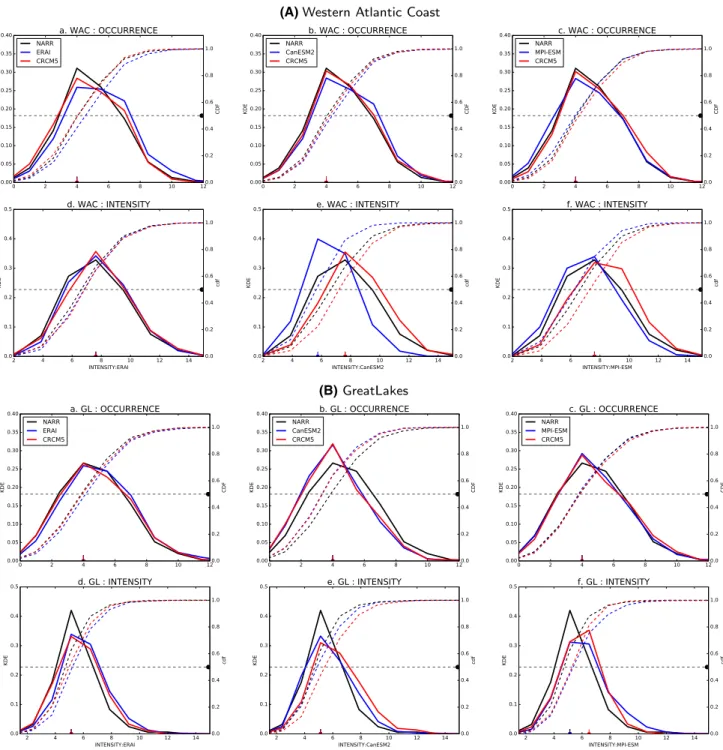
Over the WAC area (Fig. 11a), NARR occurrences range from about 0 to 12 storms per month, with a sta-tistical median and mode of around 4 storms per month. The regular regime is materialized by the compact shape of the distribution, implying that relatively small disper-sion occurs around the mean occurrence value (~5 storms per month). ERAI distribution is shifted toward the right-hand side, suggesting more presence of months with higher storm occurrence values, as suggested by the larger median (5 storms in ERAI instead of 4 in NARR). This distribu-tion shift also suggests that ERAI positive occurrence bias over the coastal area (Fig. 3) may be related to a larger than observed contribution of very active regimes, with an occurrence range of about 6–9 storms per month during the winter season. It is shown that ERAI-driven CRCM5 sig-nificantly reduces the shift of the pattern, leading to better agreement in terms of median and modes with respect to NARR. The intensity KDE shows that, in this WAC regular regime, storm intensity has a median value of ~7 CVU and is pretty well reproduced by ERAI and CRCM5 compared with the NARR distribution. It is worth adding that, even for extreme events (12–14 CVU), the RCM still behaves very well. On the other hand, MPI-ESM-LR and CanESM2 models show fair skill in reproducing the observed shape of the occurrence distribution in a manner very compara-ble to ERAI. Interestingly, it is shown that, as with ERAI, the regionally downscaled simulations can still bring some improvement, especially for a weaker occurrence regime. Finally, serious discrepancies arise in the EC intensity distribution of the CanESM2, in which a weaker storm regime dominates the distribution. The correction brought by CRCM5 is very meaningful even though there is an overestimation of higher intensity storms in return. This too-intense storm category, captured by both GCM-driven CRCM5 runs, could be linked with the SST warm biases inherited from the GCM simulations.
A point of agreement among all data sets is that storm occurrence frequencies are generally distributed over smaller values (and with weaker intensity) over the Great Lakes region (Fig. 11b) than over the WAC region. In addi-tion, the compact shape of the GL occurrence distribution is still noticeable for all datasets, although with a less regu-lar regime (see Fig. 10). ERAI and its driven CRCM5 per-form very well with respect to NARR, exhibiting a regu-lar storminess regime centered on 4 storms per month. On the other hand, although a slight improvement can be seen from CRCM5, storm intensity appears biased toward higher values in both ERAI and CRCM5 in comparison
with NARR. This means that these two models would tend to show a storm regime that is more intense than observed (between 7 and 10 CVU). More generally, over this region, it is difficult to conclude on whether CRCM5 improves both parameters in comparison with its driving data. In fact, the
regional model seems to mimic its driving dataset, leading to a systematic overestimation of the occurrence of intense storms. This is a counterintuitive outcome since one would expect the RCM to be able to capture the Great Lakes effects and therefore not to mimic the large-scale model.
(A) Western Atlantic Coast
(B) GreatLakes
Fig. 11 Kernel density estimates (KDE) of 25-year NDJFM monthly
storm parameters computed over the 4 regions delimited by blue boxes in Fig. 1: a Western Atlantic coast, b Great Lakes, c Colorado and d Alberta. Each column represents a given simulation monthly storm occurrence (storm month−1, top row) and intensity (CVU,
bot-tom row) distributions. The cumulative density function computed
from the integral of KDE is shown in dashed curves and the hori-zontal black-dashed line indicates the CDF 0.5 value. On each plot, NARR is in black, the driving data in blue and the corresponding CRCM5 run in red. On the x-axis, markers show the statistical mode values for each data set
The analysis reveals that, because of the smaller footprint of the GL effects (in opposition to the WAC), more resolu-tion and certainly more refinement in the surface coupling system are needed to “free” the RCM from its driver.
Finally, over the continental cyclogenesis regions (COL and ALB, Fig. 11c, d, respectively), the intermit-tent regime already seen in Fig. 10 is well materialized with (right-hand) long-tailed distributions for all datasets.
EC occurrence is a very dispersive process, occurring with relatively weak mean value (~2 storms per month) but marked by regimes with high occurrences (4–8 storms per month). Figure 11c, d show that the regional model tends to improve the spatio-temporal distribution of storm occur-rence and intensity with respect to ERAI and CanESM2 (and MPI-ESM-LR for the EC intensity over the Alberta area only, see Fig. 11e). On the other hand, the RCM skill
(C) Colorado
(D) Alberta
remains comparable with that of MPI-ESM-LR for the occurrence over the two regions.
Hence, in general for the majority of regions (except the Great Lakes area) and EC characteristics, the CRCM5 simulations tend to improve the occurrence and intensity of storms from their reanalysis and GCM-driven runs. Over the Great Lakes area, the RCM is more dependent on its driven conditions and the AV is less obvious or tenuous, i.e. the regional scale influences and the value added to EC features are less marked than over the other continental and maritime areas where both high-resolution topographic and land/sea boundary conditions can emerge.
5 Conclusion and future work
The paper has evaluated the value added by the Canadian Regional Climate Model—version 5 (CRCM5) when simu-lating northern American ECs as one of the major compo-nents influencing mid-latitude weather and climate states. Because complex physics at different time and space scales is involved, assessing model performance with respect to EC genesis and development requires detailed analyses, and the current paper has attempted to disentangle some of them. Thus, both seasonal characteristics and intraseasonal variability have been assessed and the main findings are: • The choice of a reference dataset for model
compari-son is an important factor for storm tracking analysis. The present analysis—in agreement with Hodges et al. (2011)—found that ERAI mostly overestimates storm genesis and occurrence (and, to a lesser extent, inten-sity) over North America with respect to the regional reanalysis. Because of these differences among reanal-yses, some results from previous studies assessing the performance of (global and regional) climate models need to be taken with caution, especially when regional-scale processes are implicated and interact strongly with large-scale flow and ECs over North America. More fundamentally, there is a need to reach a consensus on the notion of reference data. This consensus may vary depending on the applications or the diagnostic varia-bles considered (e.g. thermodynamical or diabatic forc-ings, storm tracking, etc.), and the region of interest. • The two GCM simulations capture the overall picture of
storm activity over North America, confirming results from previous studies (Zappa et al. 2013). However, systematic large biases appear over the western marked relief area where the GCM’s relatively lower height of mountains leads to an overestimate of cyclone occur-rence and intensity. This is thought to be a minor (or solvable) issue since GCM resolution will continue to increase. Near water masses (Hudson Bay, Great Lakes
and East Coast), it is clear that both parameters are underestimated. Comparison with ERAI suggests even more amplified biases over the East Coast in line with previous results. It is also surprising that, despite strong SST warm biases, GCMs—especially CanESM2—still underestimate storm genesis and intensity over the East Coast. Interestingly, Zappa et al. (2013) have shown that guiding GCMs with “observed” SST does not bring sig-nificant improvement. This lack of sensitivity over the western warm boundary current may be due to: (1) the limitation of horizontal resolution in the GCMs since it is shown that SST gradients (as well as amplitudes) need to be well resolved in both the time and space dimensions to correctly impact EC dynamics and (2) physical parametrization of surface latent and sensible heat fluxes (e.g., Bourassa et al. 2013). This last point is supported by the fact that CRCM5, even inheriting from the same (spatial and temporal resolution) SSTs, was at least able to simulate some added value over this area for both occurrence and intensity characteristics and also in terms of persistence or regularity with respect to boundary conditions. It is recalled that CRCM5 uses a weather forecast model physics, the Environment Canada Global Environmental Multiscale (GEM) fore-cast model (Côté et al. 1998a, b). This means that this regional model uses an improved physical package com-pared to GCM-scale model to resolve short term pro-cesses and high frequency turbulent fluxes. Indeed, the planetary boundary layer parameterization in the GEM forecast model has been regularly improved and modi-fied during the course of time (see a review used in the CRCM5 in Martynov et al. 2013), for example in intro-ducing turbulent hysteresis to improve the representa-tion of the synoptic scales (i.e. ECs in winter; see Zadra et al. 2012).
• CRCM5 driven by ERAI shows remarkable skill over the whole NA domain, outperforming ERAI, particu-larly near mountains (Midwest Rockies). Regional boxplots have shown that cyclone genesis, intensity and occurrence are remarkably improved with respect to NARR, showing more accurate statistics (median and quartiles) than ERAI ones. On the other hand, the dynamically downscaled simulations have revealed, with respect to GCMs, that the notion of added value is quite complex to assess since it involves, at least, resolution and physics issues. For instance, the con-tinental cyclogenesis and lysis areas (Colorado and Alberta) appeared well captured in CRCM5 while the Great Lakes region occurrence and intensity remained comparable to those provided by GCMs. However, it seems that, over the East Coast, in contrast with GCMs, SST biases impact CRCM5 performance in a more comprehensive way: positive SST biases would lead to
stronger cyclones (consistently with Booth et al. 2012). And, more generally, the sensitivity of any RCM to changes (or biases) in surface conditions is more pro-nounced than in any of the coarse scale models, due to the improved resolution of the RCM, which will bring out amplified effects of surface and low level diabatic fluxes not resolved at the scale of a GCM. Nevertheless, quite a substantial improvement has been revealed with respect to storm occurrence in the CRCM5 simulations over the WAC area, with also noticeable agreement for storm intensity in the case of CanESM2 driving simula-tion.
• In an attempt to characterize the storminess regimes within the winter season and thus the intra-seasonal var-iability, the dispersion parameters and monthly occur-rence (and intensity) distributions were assessed. It is shown with NARR (and generally by all datasets) that the eastern part of NA is subject to a persistent (regu-lar) regime while that of the western part is more inter-mittent, characterized by temporally clustered storms. Although it seems obvious that the RCM seriality is somehow imposed by boundary conditions, the disper-sion parameter shows that substantial improvement is brought by using CRCM5 over the continental cyclo-genesis regions and on to the Atlantic. The time series of monthly occurrence and intensity density function analysis over the four domains also shows that, in gen-eral, the RCM is more accurate in refining the storm activity regimes (statistical medians, mean, modes and extreme event tails for occurrence and intensity).
To sum up, the paper has confirmed the reasonable idea that an RCM is able to reproduce and improve our capacity to simulate EC characteristics in a climate per-spective. That has been demonstrated by the skill of ERAI-driven simulations, which handle extratropical storm characteristics (genesis, occurrence, intensity, dis-persion) fairly well (and partly even better than ERAI). On the other hand, the added value that an RCM brings to GCMs is tangible firstly through resolution effects and then through improved physics. In particular over the East Coast, despite largely biased boundary conditions (in the CanESM2 driven version) and despite the fact that those bias effects naturally tend to be exacerbated at higher res-olution (e.g. RCM resres-olution), the CRCM5 has revealed serious potential, mainly for improving storm intensity distribution. However, further work is needed to fully evaluate the whole potential added value for the CRCM5 versus coarse scale boundary conditions, and in particu-lar the effect of different time resolution simulations used here in the storm tracking (3 hourly for RCM and NARR while 6 hourly for the rest) on sensitive EC features (ex. storm speed and phase of rapid intensification during
explosive developments over the eastern NA coast). Fur-thermore, all data were spatially re-gridded to a com-mon 100 km horizontal grid resolution, to facilitate the comparison with an intermediate resolution between the RCM (~50 km) and GCM (~200 km). As we were mainly interested to evaluate the added value of RCM and our focus is on winter synoptic scale storms, i.e. in general with a size more often higher than 1500 km, this interpo-lation was not detrimental for RCM, but can potentially induce some artefact in GCM scale values (not neces-sarily problematic as large scale systems are concerned). Nevertheless, this needs to be evaluated in future works, i.e. to analyze to what extent those space and time differ-ences may impact the results and to be able to generalize our conclusion. Finally, considering the inherent sensitiv-ity of EC characteristics to the surface conditions in win-ter, i.e. SST gradients and location of sea-ice margin over the eastern coast of North America, further works need to be done using CRCM5 simulations with unbiased SSTs (e.g., Hernández-Díaz et al. 2016). Also, different RCMs need to be used for an in-depth evaluation of the uncer-tainties brought by the downscaling model and to develop more robust EC regional scale information over the North America region, by using various combinations of GCMs and greenhouse gas emission scenarios (GES). This work is already underway and is using different CORDEX runs with two GES to generate climate change information, the links between changes in storm track occurrence and intensity, and the modification in the precipitation and the wind regime over the coming decades. This is of par-ticular importance as ECs over eastern North America have the most pronounced effects on intense precipita-tion, including heavy snowfall events, and coastal flood risks occurring from the fall to spring months.
Acknowledgements The authors acknowledge the financial support
of the Canadian Network for Regional Climate and Weather Processes (CNRCWP—http://www.cnrcwp.uqam.ca/), funded by the Natural Sciences and Engineering Research Council of Canada (NERSC-CRSNG—http://www.nserc-crsng.gc.ca/index_eng.asp). We are also grateful to the Centre pour l’Étude et la Simulation du Climat à l’Échelle Régionale (ESCER) of the Université du Québec à Mon-tréal (UQAM) for providing the outputs of CRCM5 simulations used in our study. We specifically thank Ms Katja Winger and Prof. Laxmi Sushama at UQAM, who provided information and output files from CRCM5. We would also like to thank the CCCma/ECCC, ECMWF, NCEP and the Max-Planck Institute for providing output files for CanESM2, ERAI, NARR and MPI-ESM-LR, respectively. Finally, the authors sincerely thank the two anonymous reviewers whose con-tributions have helped to improve the results and the structure of the paper.
Open Access This article is distributed under the terms of the
Creative Commons Attribution 4.0 International License (http:// creativecommons.org/licenses/by/4.0/), which permits unrestricted use, distribution, and reproduction in any medium, provided you give appropriate credit to the original author(s) and the source, provide a
link to the Creative Commons license, and indicate if changes were made.
References
Ahrens CD (2009) Meteorology today: an introduction to weather, climate, and the environment, Brooks/Cole Edition (9th edn), Brooks Cole, Belmont, p 355
Allen JT, Pezza AB, Black MT (2010) Explosive cyclogenesis: a global climatology comparing multiple reanalyses. J Climate 23(24):6468–6484
Arora VK, Coauthors (2011) Carbon emission limits required to satisfy future representative concentration path-ways of greenhouse gases. Geophys Res Lett 38:L05805. doi:10.1029/2010GL046270
Bengtsson L, Hodges KI, Roeckner E (2006) Storm tracks and cli-mate change. J Clicli-mate 19:3518–3543
Blender R, Schubert M (2000) Cyclone tracking in different spatial and temporal resolutions. Mon Weather Rev 128:377–384 Bluestein HB, (1993) Synoptic–dynamic meteorology in midlatitudes.
In: Observations and theory of weather systems, Vol. II, Oxford University, Oxford, p 594
Booth JF, Thompson L, Patoux J, Kelly KA (2012) Sensitivity of midlatitude storm intensification to perturbations in the sea surface temperature near the Gulf Stream. Mon Weather Rev 140:1241–1256
Bourassa MA et al (2013) High-latitude ocean and sea ice surface fluxes: challenges for climate research. Bull Amer Meteor Soc 94:403–423. doi:10.1175/BAMS-D-11-00244.1
Branscome LE, Gutowski WJ Jr, Stewart DA (1989) Effect of sur-face fluxes on the nonlinear development of baroclinic waves. J Atmos Sci 46:460–475
Brayshaw DJ, Hoskins BJ, Blackburn M (2009) The basic ingredients of the North Atlantic storm track. Part I: Land–sea contrast and orography. J Atmos Sci 66:2429–2558
Chang EK, Lee S, Swanson KL (2002) Storm track dynamics. J Cli-mate 15(16):2163–2183
Colle BA, Zhang Z, Lombardo K, Liu P, Chang E, Zhang M (2013) Historical evaluation and future prediction in Eastern North America and western Atlantic extratropical cyclones in the CMIP5 models during the cool season. J. Climate. 2013; 26:6882–6903
Colle BA, Booth JF, Chang EKM (2015) A review of historical and future changes of extratropical cyclones and associated impacts along the US East Coast. Curr Clim Change Rep 1:125–143. doi:10.1007/s40641-015-0013-7
Côté J, Desmarais J-G, Gravel S, Méthot A, Patoine A, Roch M, Stan-iforth A (1998a) The operational CMC-MRB global environ-mental multiscale (GEM) model. Part II: results. Mon Weather Rev 126:1397–1418
Côté J, Gravel S, Méthot A, Patoine A, Roch M, Staniforth A (1998b) The operational CMC-MRB global environmental multiscale (GEM) model. Part I: Design considerations and formulations. Mon Weather Rev 126:1373–1395
Côté H, Grise KM, Son S-W, de Elía R, Frigon A (2015) Challenges of tracking extratropical cyclones in regional climate models, Clim Dyn 44(11):3101–3109
Dee DP et al. (2011) The ERA-Interim reanalysis: configuration and performance of the data assimilation system. Q J R Meteorol Soc 137:553–597. doi:10.1002/qj.828
Di Luca A, de Elía R, Laprise R (2015) Challenges in the quest for added value of regional climate dynamical downscaling. Curr Clim Change Rep 1(1):10–21. doi:10.1007/s40641-015-0003-9
Eichler TP, Gottschalck JA (2013) Comparison of southern Hemi-sphere cyclone track climatology and interannual variability in coarse gridded reanalysis datasets. Adv Meteorol, p 1–16 Gachon P, Saucier FJ (2003) La modélisation du climat dans les mers
intérieures du Canada : Baie d’Hudson et Golfe du Saint-Lau-rent. Nat Can 127(2):117–122
Gachon P, Saucier FJ, Laprise R (2001) Atmosphere-ocean-ice inter-action processes in the Gulf of St. Lawrence: numerical study with a coupled model. In: Sixth Conference on Polar Meteorol-ogy and Oceanography and 11th Conference on Interaction of the Sea and Atmosphere. AMS (American Meteorological Soci-ety) Meeting, San Diego (14–18 May 2001. Abstract volume, J1.18, J37–J40 (B))
Gachon P, Laprise R, Zwack P, Saucier FJ (2003) The effects of inter-actions between surface forcings in the development of a model-simulated polar low in Hudson Bay. Tellus A 55(1):61–87 Giorgi F, Jones C, Asrar GR (2009) Addressing climate information
needs at the regional level: the CORDEX framework. World Meteorol Org Bull 58:175
Goyette S, Brasseur O, Beniston M (2003) Application of a new wind gust parameterization: Multiscale case studies performed with the Canadian regional climate model. J Geophys Res 108(D13):4374. doi:10.1029/2002JD002646
Giorgetta et al (2013) Climate and carbon cycle changes from 1850 to 2100 in MPI-ESM-LR simulations for the coupled model inter-comparison project phase 5. J Adv Model Earth Syst 5:572–597. doi:10.1002/jame.20038
Grise KM, Son S-W, Gyakum JR (2013) Intraseasonal and interannual variability in North American storm tracks and its relationship to equatorial Pacific variability. Mon Weather Rev 141:3610–3625 He J, Zhang M, Lin W, Colle B, Vogelmann A (2013) Simulations of
a mid-latitude cyclone over the southern Great Plains using the WRF nested within the CESM. J Adv Mod Earth Syst 5:611–622 Hernández-Díaz L, Laprise R, Nikiéma O, Winger K. (2016) 3-Step
dynamical downscaling with empirical correction of sea-surface conditions: application to a CORDEX Africa simulation. Clim Dyn. doi:10.1007/s00382-016-3201-9
Hirsch ME, DeGaetano AT, Colucci SJ (2001) An East Coast winter storm climatology. J Clim 14:882–899
Hodges KI, Lee RW, Bengtsson L (2011) A comparison of extratropi-cal cyclones in recent reanalyses ERA-Interim, NASA MERRA, NCEP CFSR, and JRA-25. J Clim 24:4888–4906
Hoskins BJ, Hodges KI (2002) New perspectives on the Northern Hemisphere winter storm tracks. J Atmos Sci 59:1041–1061 Hoskins BJ, Valdez P (1990) On the existence of storm-tracks. J
Atmos Sci 47:1854–1864
IPCC (2013), Climate change 2013: the physical science basis. In: Stocker TF, Qin D, Plattner G-K, Tignor M, Allen SK, Boschung J, Nauels A, Xia Y, Bex V, Midgley PM (eds) Contribution of working group I to the fifth assessment report of the intergov-ernmental panel on climate change. Cambridge University, Cam-bridge, p 1535
Jung T, Gulev SK, Rudeva I, Soloviov V (2006) Sensitivity of extra-tropical cyclone characteristics to horizontal resolution in the ECMWF model. Q J R Meteorol Soc 132:1839–1857
Kumar A, Zhang L, Wang W (2013) Sea surface temperature–pre-cipitation relationship in different reanalyses. Mon Weather Rev 141:1118–1123. doi:10.1175/MWR-D-12-00214.1
Lackmann, G. (2011) Midlatitude synoptic meteorology: dynamics, analysis and forecasting, American Meteorological Society, Mas-sachusetts 345
Lambert SJ, Fyfe JC (2006) Changes in winter cyclone frequencies and strengths simulated in enhanced greenhouse warming exper-iments: results from the models participating in the IPCC diag-nostic exercise. Clim Dyn 26:713–728