Structural Characterization of Highly Flexible Proteins by Small-Angle Scattering.

(1)

HAL Id: hal-01664316

https://hal.laas.fr/hal-01664316

Submitted on 14 Dec 2017

HAL is a multi-disciplinary open access

archive for the deposit and dissemination of sci-entific research documents, whether they are pub-lished or not. The documents may come from teaching and research institutions in France or abroad, or from public or private research centers.

L’archive ouverte pluridisciplinaire HAL, est destinée au dépôt et à la diffusion de documents scientifiques de niveau recherche, publiés ou non, émanant des établissements d’enseignement et de recherche français ou étrangers, des laboratoires publics ou privés.

Structural Characterization of Highly Flexible Proteins

by Small-Angle Scattering.

Tiago Cordeiro, Fatima Herranz-Trillo, Annika Urbanek, Alejandro Estaña,

Juan Cortés, Nathalie Sibille, Pau Bernadó

To cite this version:

Tiago Cordeiro, Fatima Herranz-Trillo, Annika Urbanek, Alejandro Estaña, Juan Cortés, et al.. Struc-tural Characterization of Highly Flexible Proteins by Small-Angle Scattering.. Advances in Exper-imental Medicine and Biology, Kluwer, 2017, pp.PP.107-129. �10.1007/978-981-10-6038-0_7�. �hal-01664316�

(2)

Structural Characterization of Highly Flexible Proteins by

Small-‐Angle Scattering

Tiago N. Cordeiroa_{,
Fátima
Herranz-‐Trillo}a,c_{,
Annika
Urbanek}a_{,
Alejandro
Estaña}a,b_{,
Juan} Cortésb_{,
Nathalie
Sibille}a_{,
Pau
Bernadó}a,_*

a-‐Centre de Biochimie Structurale. INSERM U1054, CNRS UMR 5048, Université de Montpellier. 29, rue de Navacelles, 34090-‐Montpellier, France.

b-‐ LAAS-‐CNRS, Université de Toulouse, CNRS, Toulouse, France.

c-‐ Department of Pharmacy and Department of Drug Design and Pharmacology, University of Copenhagen, Universitetsparken 2, 2100 Copenhagen, Denmark.

Contact Author: Pau Bernadó (pau.bernado@cbs.cnrs.fr). Tel. +33 467417705

Keywords: Intrinsically Disordered Proteins, Small-‐Angle X-‐ray Scattering, Small-‐angle Neutron Scattering, Ensemble Methods, Protein-‐Protein Interactions, Nuclear Magnetic Resonance, Low-‐Complexity Regions, Random Coil Models, Amyloids.

(3)

Abstract:

Intrinsically Disordered Proteins (IDPs) are fundamental actors of biological processes. Their inherent plasticity facilitates very specialized tasks in cell regulation and signalling, and their malfunction is linked to severe pathologies. Understanding the functional role of disorder requires the structural characterization of IDPs and the complexes they form. Small-‐angle Scattering of X-‐rays (SAXS) and Neutrons (SANS) have notably contributed to this structural understanding. In this review we summarize the most relevant developments in the field of SAS studies of disordered proteins. Emphasis is given to ensemble methods and how SAS data can be combined with computational approaches or other biophysical information such as NMR. The unique capabilities of SAS enable its application to extremely challenging disordered systems such as low-‐complexity regions, amyloidogenic proteins and transient biomolecular complexes. This reinforces the fundamental role of SAS in the structural and dynamic characterization of this elusive family of proteins.

(4)

INTRODUCTION

Intrinsically disordered Proteins or Regions (IDPs/IDRs) have emerged as key actors for a large variety of biological functions such as cell signalling and regulation (Kriwacki et al., 1996; Wright and Dyson, 1999; Dunker et al., 2002; Wright and Dyson, 2015). The main feature of IDPs and IDRs is their lack of permanent secondary or tertiary structure that provides them with an inherent malleability enabling highly specialized biological functions (Dunker et al., 2002). Eukaryotic genomes are highly enriched in genes coding for disordered proteins, and this observation has been linked to the major complexity of these organisms. The capacity of IDPs to adapt their conformation to specifically recognize one or several partners, and the low to moderate affinity for partners make IDPs ideal for protein-‐ protein interactions (Tompa et al., 2015). In fact, it has been shown that interactome hubs are enriched in this family of proteins (Dunker et al., 2005; Kim et al. 2008). Partner recognition is normally performed through conserved and partially structured motifs of the protein, and their individual properties can be modulated by post-‐translational modifications or alternative splicing. IDRs are highly flexible regions connecting well-‐folded globular proteins forming the so-‐called multi-‐domain proteins. Multi-‐domain protein topology, which is highly prevalent in eukaryotes, enables the presence of multiple biological activities performed by the globular domains in close proximity (Hawkins and Lamb 1995; Levitt, 2009). In many of these cases, IDRs behave as entropic linkers with an inherent plasticity that can be tuned depending on the length and the specific amino acid sequence of the region.

The biological relevance of IDPs has fostered their structural characterization (Eliezer 2009). Identification of the conformational preferences of binding motifs, the detection of transient long-‐range contacts within the chain, the structural perturbations exerted by PTM, the shape of biomolecular complexes with disordered partners, and the spatial distribution of globular domains in multi-‐domain protein are structural features that must be characterized to understand the molecular bases of biological function. This characterization is far from being trivial as the inherent disorder of IDPs/IDRs precludes their crystallization. Nuclear Magnetic Resonance (NMR) has become the only technique that can provide atomic-‐ resolution information on IDPs (Dyson and Wright, 2004). Novel NMR experiments and modelling strategies have been developed to interpret experimental parameters in terms of structure (Jensen et al., 2009; Jensen et al., 2013; Jensen et al., 2014; Wright and Dyson,

(5)

2015). However, some structural aspects that remain elusive by NMR such as the overall shape and size of disordered proteins or the distribution of interdomain position in multi-‐ domain proteins.

Small-‐Angle Scattering (SAS) of X-‐rays (SAXS) or Neutrons (SANS) have emerged as powerful techniques to probe the structure and dynamics of biomolecules in solution at low resolution (Figin and Svergun, 1987; Svergun and Koch, 2003; Koch et al., 2003; Putnam et al. 2007; Jacques and Trewhella, 2010). SAS provides unique information about the overall size and shape of individual macromolecules or their complexes in a rapid manner. Additionally, structural changes upon environmental perturbations, such as interactions with other molecules, can be addressed straightforwardly. Major advances in instrumentation and computational methods in the last decade have led to a tremendous increase in the applications of SAS in structural biology (Petoukhov and Svergun, 2007; Mertens and Svergun, 2010; Pérez and Nishioni, 2012; Rambo and Tainer, 2013; Graewert and Svergun, 2013). One of the major advances of SAXS in the last decade has been its extension to address biomolecular dynamics (Doniach, 2001; Bernadó and Svergun, 2012a; Receveur-‐Brechot and Durand, 2012; Bernadó and Svergun, 2012b; Kikhney and Svergun, 2015; Kachala et al., 2015). Although used in the past to study protein flexibility (Aslam et al., 2003), the availability of robust protocols to interpret SAS data in terms of ensembles of conformations have generalized these studies and, therefore, have enriched the spectrum of applications of the technique (Bernadó and Blackledge, 2010).

The aim of this chapter is to provide an overview of the recent developments of SAS to study highly disordered proteins. A special emphasis is put on biological scenarios involving highly flexible proteins for which SAS is a crucial tool to tackle the structural/dynamic bases of biological function.

Scattering properties of IDPs

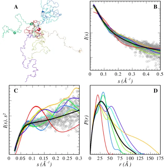
The fact that IDPs sample an astronomical number of conformations has a strong impact on the scattering profiles measured and their comprehensive analysis in terms of structure. The experimental SAXS profile of an IDP corresponds to the average of all the conformations that the protein adopts in solution, inducing special features to the curves. Figure 1A displays the synthetic SAXS curves for seven conformations of p15PAF_{,
a
111
residue-‐long
IDP,
selected} from a large pool of 5,000 (De Biasio et al., 2014). The individual conformations display

(6)

several features along the complete momentum transfer range simulated. The initial part of the simulated curves, containing the lowest resolution structural information, presents distinct slopes indicating a large variety of possible sizes and shapes that an unstructured chain can adopt. The SAXS profile, obtained after averaging curves for the 5,000 conformations, presents a smoother behavior with essentially no features (Fig. 1B).

Figure 1. (A) Seven representative conformers randomly selected from an ensemble of 5,000 explicit all-‐atoms models generate for p15PAF_{(De
Biasio
et
al.,
2014).
Solid
lines
correspond}

to their computed SAXS curves (B) and Kratky plots (C) and are colored as in planel A. T. The average over the ensemble of 5,000 conformations yields a featureless curve that is in very good agreement with the experimental data (gray circles). (D) p(r) functions computed for the 7 conformers and the complete ensembles in the same color code that in panels (A-‐C).

Traditionally, Kratky plots (I(s)·s2_{as
a
function
of
s)
have
been
used
to
qualitatively
identify} disordered states and distinguish them from globular particles. The scattering intensity of a

(7)

globular protein behaves approximately as 1/s4_{conferring
a
bell-‐shaped
Kratky
plot
with
a} well-‐defined maximum. Conversely, an ideal Gaussian chain has a 1/s2_{dependence
of
I(s)} and therefore presents a plateau at large s values. In the case of a chain with no thickness, the Kratky plot also presents a plateau over a specific range of s, which is followed by a monotonic increase. This last behavior is normally observed experimentally in unfolded proteins. The Kratky representation has the capacity to enhance particular features of scattering profiles that allows an easier identification of different degrees of compactness (Doniach, 2001). This is shown in figure 1C where different degrees of compactness for the conformations are observed. Multi-‐domain proteins present in the same molecule a dual (folded/disordered) behavior consequently SAXS profiles and Kratky plots present contributions from both structurally distinct regions. Pair-‐wise distance distributions, p(r), derived from disordered proteins also present specific properties (Figure 1D). The most characteristic feature is the smooth decrease towards large intramolecular distances. Maximum intramolecular distance, Dmax, which represents the maximum distance within one

of the accessible conformations of the protein, are very large in disordered proteins. It is worth noting that due to the low population of highly extended conformations in the ensembles, experimental Dmax values are systematically underestimated (Bernadó, 2010).

Unstructured proteins, due to the presence of extended conformations, are characterized by large average sizes compared to globular proteins. The radius of gyration, Rg, which can be

directly obtained from a SAXS curve using a classical Guinier approximation, is the most common descriptor to quantify the overall size of molecules in solution (Guinier, 1939). In the Guinier approximation, it is assumed that at very small angles (s < 1.3/Rg) the scattering

intensity can be represented as I(s) = I(0) exp(-‐(sRg)2/3), and the Rg is obtained by a simple

linear fit in logarithmic scale. Debye’s approximation (eq. 1) can be more precise than Guinier’s one to derive Rg values as its validity extends to larger momentum transfer ranges

(Calmettes et al., 1994).

(

x

)

2 x 1 e x 2 ) 0 ( I ) s ( I − + − = ; x = s2·Rg2 (1)

Alternatively, p(r) function calculated from the complete scattering profile using a Fourier transformation also yields precise Rg values for disordered proteins.

(8)

The experimental Rg is a single value representation of the size of the molecule, which for

disordered states represents a z-‐average over all accessible conformations in solution (Feigin and Svergun, 1987). The most common quantitative interpretation of Rg for unfolded

proteins, which is based on Flory’s studies in polymer science, relates this parameter to the length of the protein chain through a power law (Flory, 1953),

Rg = R0·Nν (2)

where N is the number of residues in the polymer chain, R0 is a constant that depends on several factors, in particular, on the persistence length, and ν is an exponential scaling factor. For an excluded-‐volume polymer, Flory estimated ν to be ≈ 0.6, and more accurate theoretical estimates established a value of 0.588 (LeGuillou and Zinn-‐Justin, 1977). A recent compilation of Rg values measured for 26 chemically denatured proteins sampling broad

range of chain lengths found a ν value of 0.598 ± 0.028, and a R0 value of 1.927 ± 0.27 (Kohn et al., 2004). The agreement between the ν value obtained experimentally and the theoretical models suggest the random coil nature of the chemically denatured proteins. However, the question whether the conformational sampling in the chemically denatured state is equivalent to that found for IDPs in native conditions must be clarified (Stumpe and Grubmüller, 2007 and references therein). Using atomistic ensemble models of several disordered proteins, Flory’s equation has been parametrized for IDPs (Bernadó and Blackledge, 2009):

Rg = (2.54 ± 0.01)·N(0.522 ± 0.01) (3)

The exponential value obtained from the parametrization, ν=0.522±0.01, is notably smaller than that derived from the dataset of denatured proteins, ν=0.598 ± 0.028, indicating that IDPs are more compact than chemically denatured proteins. This observation is in line with NMR studies that indicated that urea denatured proteins have an enhanced sampling (around 15%) of extended conformations compared with IDPs (Meier et al., 2007).

(9)

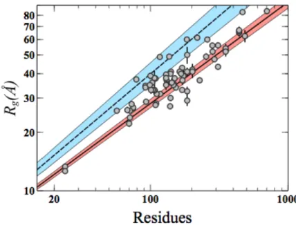
Here, we have collected Rg data from 74 IDPs from the literature (Table 1) that are plotted as

a function of the chain length (Fig. 2). As expected, the Rgs collected display a correlation

with the number of residues of the chain. This linear relationship is closer to the above-‐ mentioned parametrization of IDPs than to that established for chemically denatured proteins. As some IDPs are expected to have certain populations of secondary or tertiary structure, this relationship can be used as an interpretative tool. Thus, deviations from expected IDP random coil model indicate enhanced degrees of compactness or extendedness within the protein.

Figure 2. Rg values from Table 1 (gray dots) as a function of the number of residues are plotted in

Log-‐Log scale. Straight lines correspond to Flory’s relationships parametrized for denatured proteins (blue-‐dashed) (Kohn et al., 2004) and IDPs (red-‐solid) (Bernadó and Blackledge, 2009). Colored bands correspond to uncertainty of the parametrization for both models. Some IDPs are

not fully disordered and are globally more extended or more compact than expected for a random coil. These structural features even if transient affect the experimental Rg.

(10)

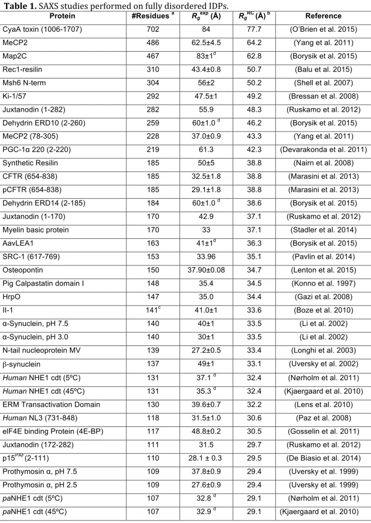
Table 1. SAXS studies performed on fully disordered IDPs.

Protein #Residues a Rgexp (Å) RgRC (Å) b Reference

CyaA toxin (1006-1707) 702 84 77.7 (O’Brien et al. 2015)

MeCP2 486 62.5±4.5 64.2 (Yang et al. 2011)

Map2C 467 83±1d 62.8 (Borysik et al. 2015)

Rec1-resilin 310 43.4±0.8 50.7 (Balu et al. 2015)

Msh6 N-term 304 56±2 50.2 (Shell et al. 2007)

Ki-1/57 292 47.5±1 49.2 (Bressan et al. 2008)

Juxtanodin (1-282) 282 55.9 48.3 (Ruskamo et al. 2012)

Dehydrin ERD10 (2-260) 259 60±1.0 d 46.2 (Borysik et al. 2015)

MeCP2 (78-305) 228 37.0±0.9 43.3 (Yang et al. 2011)

PGC-1α 220 (2-220) 219 61.3 42.3 (Devarakonda et al. 2011)

Synthetic Resilin 185 50±5 38.8 (Nairn et al. 2008)

CFTR (654-838) 185 32.5±1.8 38.8 (Marasini et al. 2013)

pCFTR (654-838) 185 29.1±1.8 38.8 (Marasini et al. 2013)

Dehydrin ERD14 (2-185) 184 60±1.0 d 38.6 (Borysik et al. 2015)

Myelin basic protein 170 33 37.1 (Stadler et al. 2014)

AavLEA1 163 41±1d 36.3 (Borysik et al. 2015)

SRC-1 (617-769) 153 33.96 35.1 (Pavlin et al. 2014)

Osteopontin 150 37.90±0.08 34.7 (Lenton et al. 2015)

Pig Calpastatin domain I 148 35.4 34.5 (Konno et al. 1997)

HrpO 147 35.0 34.4 (Gazi et al. 2008)

II-1 141c 41.0±1 33.6 (Boze et al. 2010)

α-Synuclein, pH 7.5 140 40±1 33.5 (Li et al. 2002)

α-Synuclein, pH 3.0 140 30±1 33.5 (Li et al. 2002)

N-tail nucleoprotein MV 139 27.2±0.5 33.4 (Longhi et al. 2003)

β-synuclein 137 49±1 33.1 (Uversky et al. 2002)

Human NHE1 cdt (5ºC) 131 37.1 d 32.4 (Nørholm et al. 2011)

Human NHE1 cdt (45ºC) 131 35.3 d 32.4 (Kjaergaard et al. 2010)

ERM Transactivation Domain 130 39.6±0.7 32.2 (Lens et al. 2010)

Human NL3 (731-848) 118 31.5±1.0 30.6 (Paz et al. 2008)

elF4E binding Protein (4E-BP) 117 48.8±0.2 30.5 (Gosselin et al. 2011)

p15PAF(2-111) 110 28.1 ± 0.3 29.5 (De Biasio et al. 2014)

Prothymosin α, pH 7.5 109 37.8±0.9 29.4 (Uversky et al. 1999)

Prothymosin α, pH 2.5 109 27.6±0.9 29.4 (Uversky et al. 1999)

paNHE1 cdt (5ºC) 107 32.8 d 29.1 (Nørholm et al. 2011)

(11)

N-protein of bacteriophage λ 107 33±2 e 29.1 (Johansen et al. 2011a)

N-protein of bacteriophage λ 107 38±3.5 29.1 (Johansen et al. 2011b)

Human NCBD domain 105 33±1 28.8 (Borysik et al. 2015)

FEZ1 monomer 103 36±1 28.5 (Alborghetti et al. 2010)

HIV-1 Tat133 101 33.0±1.5 28.3 (Foucault et al. 2010)

Human Calpastatin (137-237) 100 39.0±1.5 28.1 (Borysik et al. 2015)

p53 (1-93) 93 28.7±0.3 27.1 (Wells et al. 2008)

Sic1 92 34.7 26.9 (Mittag et al. 2010)

pSic1 (hexaphosphorylated) 92 34.0 26.9 (Mittag et al. 2010)

Juxtanodium (103-282) 79 37.4 38.1 (Ruskamo et al. 2012)

PIR domain 75 26.5±0.5 24.2 (Moncoq et al. 2004)

N-term NRG1 type III 75 26.8 d 24.2 (Chukhlieb et al. 2015)

IB5 73 b 27.9±1.0 23.8 (Boze et al. 2010)

ACTR (5ºC) 71 25.8 d 23.5 (Kjaergaard et al. 2010)

ACTR (45ºC) 71 23.8 d 23.5 (Kjaergaard et al. 2010)

PaaA2 (1-63) 70 a 22.15±0.87 d 23.3 (Sterckx et al. 2014)

N-term VS Virus phosphoprotein 68 26±1 f 23.0 (Leyrat et al. 2011)

E3 ubiquitin ligase RNF4 (32-82) 57 25.8 21.0 (Kung et al. 2014)

Histatin 5 24 13.3 13.3 (Cragnell et al. 2016)

R/S peptide 24 12.6±0.1 13.3 (Rauscher et al. 2015)

Constructions of Tau Protein

Tau ht40 441 65±3 61.0 (Mylonas et al. 2008)

Tau K32 202 42±3 40.6 (Mylonas et al. 2008)

Tau ht23 352 53±3 54.2 (Mylonas et al. 2008)

Tau K32 AT8 AT100 202 41±3 40.6 (Mylonas et al. 2008)

Tau ht23 S214E 352 54±3 54.2 (Mylonas et al. 2008)

Tau ht23 AT8 AT100 352 52±3 54.2 (Mylonas et al. 2008)

Tau K18 P301L 130 35±2 32.2 (Mylonas et al. 2008)

Tau ht40 AT8 AT100 PHF1 (10ºC) 441 66±3 61.0 (Shkumatov et al. 2011)

(12)

a-‐ When present, purification tags or extra terminal residues resulting from cloning were considered as part of the protein

b-‐ Threshold Rg value obtained from the parametrization of Flory’s relationship with the coil database. c-‐ Length of the most populated isoform of the samples was used.

d-‐ Rg derived from averaging conformations selected with EOM.

e-‐ Data measured by SANS in highly crowded conditions (130 mg/ml of BPTI) f-‐ Data derived from the 10mM Arg/Glu buffer.

(13)

Molecular Modelling of Intrinsically Disordered Proteins

The interpretation of the SAXS parameters such as Rg, p(r) and Dmax from disordered

proteins in terms of structure is limited to overall molecular information. In order to fully exploit the structural and dynamic information encoded in SAXS data, the use of realistic three-‐dimensional models is necessary. However, the generation of conformational ensembles of disordered proteins is extremely challenging (Zhou, 2004). IDPs present a relatively flat (non-‐funnelled) energy landscape, with an extremely large number of local minima separated by low-‐energy barriers. This, combined with their large size, makes the analysis of their energy landscape a challenging problem for computational methods. Most of the available computational methods aim at collecting an ensemble representation of IDPs (Bernadó et al., 2007; Jensen et al., 2014; Wright and Dyson, 2015). This requires an extensive and statistically correct exploration of the conformational space to obtain a representative set of states. Three main families of approaches have been proposed to generate conformational ensembles: molecular dynamics (MD) simulations, Monte Carlo (MC) methods, and experimentally parametrized statistical approaches. These three families of methods are succinctly explained next.

MD simulations analyze the evolution of the system under study by solving Newton's equations of motion (Karplus and McCammon, 2002; Piana et al., 2014). Theoretically, MD is a suitable method to correctly sample the conformational space of IDPs. Nevertheless, in practice, the high-‐dimensionality and the wideness of the energy landscape hampers its exhaustive exploration. Several approaches have been proposed to enhance conformational exploration with MD methods. A particularly effective one is Replica Exchange MD (REMD) that runs multiple simulations in parallel with different settings (usually different temperatures) and exchanges states between these processes (Trakawa and Takada, 2011; Zerze GH et al. 2015; Chebaro et al., 2015). Going further in this direction, a very recent method called Multiscale Enhance Sampling (MSES) couples temperature replica exchange and Hamiltonian replica exchange, using a coarse-‐grained model to guide atomistic conformational sampling (Lee KH et al., 2016). The performance of MD-‐based method can also be improved by the integration of experimental data to restrain the exploration of the most relevant regions of the conformational space (Lindorff-‐Larsen et al., 2004; Dedmon et al., 2005; Wu et al., 2009).

(14)

(Metropolis et al., 1953) the most widely used sampling technique (Vitalis and Pappu, 2009). The system is randomly perturbed and the new conformation is accepted with a probability that depends on the energy change between the new conformation and the previous one. Particular mention deserves a recently proposed variant called Hamiltonian Switch Metropolis Monte Carlo (HS-‐MMC), which has been specially conceived to study IDRs tethered to globular domains. Proteins including IDRs present energy minima due to the contact of the disordered and ordered regions. To avoid being trapped in such minima, the HS-‐MMC switches between an all-‐atom Hamiltonian to an excluded volume Hamiltonian to push the IDR away from the ordered domain.

Both, MD-‐based and MC-‐based approaches may suffer from inaccuracies of current energy models, which are better suited to globular proteins, and tend to provide structurally biased ensembles that do not properly reflect the conformational behaviour in solution of unstructured proteins (Best et al., 2014; Henriques et al., 2015). The development of more suitable force-‐fields and solvation models for IDPs are key issues for a correct performance of computational methods (Vitalis and Pappu, 2009b; Emperador et al., 2015).

Knowledge-‐based statistical approaches are an alternative to physics-‐based energy functions. The most representative knowledge-‐based method for the generation of atomistic models of disordered proteins is Flexible-‐Meccano (FM) (Bernadó et al., 2005; Ozenne et al., 2012), although other similar methods have been described (Jha et al., 2005). The FM algorithm uses an amino acid-‐specific statistical coil derived from crystallographic structures. In FM, each conformation is built by assembling peptide plane units in a consecutive manner using a residue-‐specific coil library derived from crystallographic structures. To avoid the collapse of the chain, a coarse-‐grained description of side chains is also used. Based on this set of conformations, experimentally measurable NMR parameters and SAXS curves can be estimated, which has permitted the validation of the resulting models (see below).

Despite the efforts that have been made to precisely describe the conformational states of disordered proteins, there are still many technical and conceptual issues that must be addressed to correctly describe their energy landscape and, as a consequence, their associated experimental observables.

(15)

IDPs sample a large number of conformations. Therefore, ensembles of conformations are the most appropriate framework to structurally represent this family of proteins. In recent years, structural biologists have addressed the challenge of describing dynamic systems in terms of ensembles of reliable conformations guided by experimental data that represents average values for the complete ensemble of conformations (Bernadó and Blackledge, 2010). SAXS has not been exempt from this tendency and several approaches have been developed to characterize protein mobility: Ensemble Optimization Method (EOM) (Bernadó et al., 2007; Tria et al., 2015), Minimal Ensemble Search (MES) (Pelikan et al., 2009), Basis-‐Set Supported SAXS (BSS-‐SAXS) (Yang et al., 2010), Maximum Occurrence (MAX-‐Occ) (Bertini et al., 2010), Ensemble Refinement of SAXS (EROS) (Rozicky et al.,2011 ), Broad Ensemble Generator with Re-‐weighting (BEGR) (Daughdrill et al., 2012), and Bayesian Ensemble SAXS (BE-‐SAXS) (Antonov et al., 2016). These methods are based on a common strategy that consists of three consecutive steps: (i) computational generation of a large ensemble describing the conformational landscape available to the protein, (ii) computation of the theoretical SAXS curves from the individual conformations, and (iii) selection of a subensemble of conformations that collectively describes the experimental profile using multiparametric optimization methods. Despite the common philosophy, these programs present distinct features in the three steps. Readers are referred to the original articles for a detailed description of the approaches.

The availability of ensemble methods has revolutionized the study of flexible proteins by SAS. Ensemble methods provide a description in terms of statistical distributions of structural parameters or conformations that represents a crucial step forward with respect to traditional analysis based on averaged parameters extracted from raw data such as Rg or

Dmax. In that context, conformational perturbations exerted by temperature (Shkumatov et

al. 2011; Kjaergaard et al., 2010), buffer composition (Leyrat et al., 2011), or mutations (Stott et al., 2010) can be monitored in terms of ensembles o accessible conformations. The main approximation of ensemble methods is the discrete description of entities that probe an astronomical number of conformations. It is therefore reasonable to argue about the real meaning of the SAXS-‐derived ensembles. An additional problem is the statistically significant size of the derived ensembles based on experimental data with a very limited amount of information (Hammel, 2012; Yang, 2014). The described strategies use distinct philosophies to address these issues. In some cases such as EOM 2.0 and MES, programs

(16)

search for the minimal number of conformations required to describe the data to limit or abolish over-‐fitting. BSS-‐SAXS and BE-‐SAXS use Bayesian statistics to address the confidence of the derived populations. In other cases, such as EROS and BEGR, populations of the conformers of an initially built ensemble are slightly modified (re-‐weighted) in order to describe the data.

SAXS-‐derived ensembles are representations of the conformational landscape sampled by proteins in solution, but not necessarily the exact states. Ensemble approaches are inherently ill-‐defined problems, and this is especially severe in SAXS that codes for a very limited amount of structural information. In that sense, it is more adequate to represent highly flexible proteins as distributions of accessible structural parameters such as Rg or

Dmax. These representations are less prone to over-‐fitting artifacts (Bernadó et al., 2007).

In disordered proteins, SAS reports on the overall size and shape of the protein in solution. The presence of extendedness or compactness can be probed by SAS, but regions causing these structural biases can not be identified unambiguously due to the low-‐resolution nature of the data. An interesting way to enrich the structural content of SAXS data to more precisely localize partially structured regions in IDPs has been proposed. In this strategy, SAXS curves are measured for multiple deletion mutants of the disordered chain, and simultaneously fitted in terms of a common ensemble. Note that this strategy is only valid if the structural elements of the full-‐length protein remain intact in the deletion mutants. This approach is described in detail in the original article of EOM where it was applied to a flexible multi-‐domain kinase (Bernadó et al., 2007). The most notable example of this approach was the study of two isoforms of Alzheimer-‐related tau, ht23 and ht40 (Mylonas et al., 2008). SAXS data for full-‐length ht23 and ht40 and for 5 and 3 deletion mutants for each isoform were measured, respectively. The simultaneous fit of all curves with EOM unambiguously identified the so-‐called repeat region as the source of residual secondary structure in tau. For the ht23 isoform, with three repeats, the maximum separation is found within the repeat domain itself. Conversely, the ht40 isoform, with four repeats, presented an enhanced separation between the repeat domain and the preceding region. These results suggest that the different number of turns (one per repeat) may lead to different global arrangements of the chain in that region.

In addition of the previously described strategy, the information content of SAXS curves measured for IDPs can be enriched with data from other techniques. NMR is by far the most

(17)

common technique used synergistically with SAXS (Sibille and Bernadó, 2012), and a special section of this chapter is devoted to it. Additionally, experimental data coming from Electron Paramagnetic Resonance (EPR) and single molecule Fluorescence Resonance Energy Transfer (smFRET) have been synergistically used with SAXS to characterize disordered proteins (Boura et al., 2012). In that sense, the development of robust ways to integrate other biophysical measurements in ensemble approaches is an unavoidable future direction.

Application of SANS to study IDPs

The physical bases and the structural information that can be derived form SAXS and SANS are equivalent and, in principle, both techniques can be used to characterize biomolecules. The more general use of SAXS is based on its higher sensitivity and the more widespread availability of beam-‐lines. SANS however offers some advantages with respect to SAXS. The first one is the absence of radiation damage that makes it a non-‐destructive technique. The second one is based on the possibility to perform contrast-‐match experiments, where some components of the sample are made invisible by finely tuning the degree of deuteration of sample components and the ratio of H2O/D2O of the buffer. Contrast matching has been widely used in structural biology and the reader is refereed to the excellent reviews available on the subject (Jacrot, 1976; Heller, 2010; Gabel, 2012).

Although SANS has been used to study IDPs or IDRs (Krueger et al., 2011) or radiation sensitive systems (Greving et al., 2010; Stanley et al., 2011; Perevozchikova et al., 2014), its main application is in contrast-‐match experiments. An example of this family of experiments is the study of the interaction of β-‐amyloid (1-‐40) with the detergent SDS (Jeng et al., 2006). In this study the use of deuterated SDS in SANS experiments enabled the characterization of the peptide in the presence of SDS and showed that β-‐amyloid adopts a short rod-‐like shape. Interestingly the authors observed that SDS suppress fibrils by forming complexes with a 30:1 molar ratio between detergent and protein.

IDPs may be particularly sensitive to the effects of molecular crowding, and contrast-‐ matching SANS experiments is a powerful tool to study these effects. By choosing appropriate levels of deuteration of the protein of interest and the crowding agent, the scattering contribution of the latter can be made negligible, enabling the study of the structural perturbations exerted by macromolecular crowding on disordered proteins. This strategy was used to study the disordered N-‐protein of bacteriophage λ in the presence of

(18)

high concentrations of bovine pancreatic trypsin inhibitor (BPTI), a small globular protein (Johansen et al., 2011a; Goldenberg and Argyle, 2014). In 46% D2O, high concentrations of non-‐deuterated BPTI were contrast matched, and only the signal of the 85% deuterated N-‐ protein was visible. The study demonstrated that molecular crowding exerted a compaction effect on N-‐protein. However, this effect was non-‐linear and the effects observed at 65 mg/mL of BPTI were equivalent to those at 130 mg/mL.

SAXS studies of IDPs within macromolecular assemblies

Given the structural plasticity of disordered proteins, they are regarded as interacting specialists and have a special place in cell signalling using short motifs or domain-‐sized disordered segments for partner recognition (Wright and Dyson, 2015; Tompa et al., 2015). Providing a comprehensive description of the biomolecular recognition processes for IDPs is thus of great importance for the understanding of key biological functions that are orchestrated by this family of proteins. In this regard, SAXS is emerging as an extremely valuable tool for characterizing biomolecular interactions involving highly flexible proteins, which are highly challenging for crystallography. The application of solution NMR also encounters severe limitations when characterizing large biomolecular complexes. Conversely, SAXS, which is not limited by size, offers a source of structural and dynamic information that by itself or combined with NMR and/or X-‐ray crystallography is a promising alternative for the structural characterization of highly dynamic proteins and complexes in solution.

The binding of an IDP to its target produces specific SAXS signatures that enable the detection the interaction. Typically, the mixing of two interacting partners will result in a rise of Rg values, otherwise, if the proteins do not form a complex the Rg value will follow an

population-‐weighted average of the two. Insightful information can be obtained by inspecting the p(r) function in the absence and presence of the disordered interaction partner. The scattering of globular proteins generally give a symmetrical bell-‐shaped p(r) function, while the interaction with a sufficiently large IDP results in tailing of the peak shape to higher values of r, culminating at a large Dmax. The Kratky and Porod-‐Debye

analyses are also powerful indicators of flexibility within macromolecular assemblies (Rambo and Tainer 2011).

(19)

It is possible to define 3D molecular envelopes describing the low-‐resolution shapes of flexible macromolecular assemblies involving IDPs (Longhi et al., 2003; Marsh et al., 2010; Gosselin et al., 2011; Devarakonda et al., 2011). However, the resulting fixed low-‐resolution structure is not the most appropriate structural description of a disordered protein. Ensemble analysis of explicit or coarse-‐grained models should provide a more accurate characterization of flexible macromolecular assemblies, particularly if combined with available structure coordinates of folded-‐domains and data affordable by NMR. Moreover, weak or moderate affinities are a hallmark of many IDP molecular recognition events, which entails the presence of multiple species in solution at standard experimental concentrations. In these cases, any modeling strategy envisioned should account for this species polydispersity to reliably describe SAS data.

Several SAXS studies have been devoted to the interactions of different IDPs with other proteins _{or
DNA,
as
the
only
source
of
structural
information
or
in
combination
with
high-‐} resolution methods. Some examples will be presented.

The complex of Msh2 and Msh6 recognizes mismatched bases in DNA during mismatch repair. The N-‐terminal region of Msh6, a 304 residue long IDR, recognizes PCNA, a protein that controls processivity of DNA polymerases. Shell and co-‐workers have demonstrated this direct interaction with SAXS (Shell et al., 2007). A comparison of the Rg, Kratky plots and p(r)

functions of the isolated partners and the complex showed that PCNA does not induce substantial structure to the N-‐terminal region of Msh6, which remains mainly disordered and proteolytically accessible upon binding. The interaction of the Msh2-‐Msh6 complex with PCNA was also addressed by SAXS. The interaction was shown to produce a complex that could be considered as a highly flexible dumbbell where both globular domains are tethered by the N-‐terminal Msh6 fragment that acts as a molecular leash. These observations were further confirmed in an additional experiment with a biologically active deletion mutant of Msh6 containing a notably shorter N-‐terminal tail. Under these conditions the important size changes upon binding were easily monitored using the p(r) and Dmax.

The tumor suppressor p53 is a multifunctional protein that plays a crucial role in processes like apoptosis control and DNA repair. P53 is a homotetramer with two folded domains that are tethered and flanked by unstructured regions. Rigid-‐body modeling of SAXS data measured for p53 suggests that the protein is a rather open cross-‐like tetrameric assembly,

(20)

which collapses to tightly embrace DNA (Tidow et al., 2007). This is how the flexibility of IDPs helps the protein to fulfill its function.

Nuclear receptors (NR) are engaged in gene transcription regulation in response to binding of specific ligands. Signal transduction from ligand binding to gene expression requires the recruitment of co-‐regulator proteins. Most NR co-‐regulators function as flexible scaffolds for chromatin modifiers and transcriptional machinery (Millard et al., 2013). Structural analyses of their interaction have been restricted to small peptides of the regulators and the nuclear receptor ligand-‐binding domain. More recently, several SAXS studies have provided new insights into the stoichiometry and binding mode of the complexes formed by NR and disordered co-‐regulators (Jin et al., 2008; Rochel et al., 2011; Devarakonda et al., 2011; Pavlin et al., 2014).

β-‐thymosin/WH2 (β-‐t/WH2) domains are widespread short disordered regions (25-‐50 residues) able to recognize G-‐actin and regulate actin-‐assembly. When bound to G-‐actin the N-‐terminal half of β-‐t/WH2 adopts a well-‐ordered amphipathic helix. SAXS analysis at different ionic strengths revealed that the C-‐terminal regions of different β-‐t/WH2 domains display distinct dynamics, which correlate with functional differences. At low ionic strength β-‐t/WH2 sequesters G-‐actin in a polymerization incompetent state, where the dynamic interactions of the C-‐terminal part are restrained to a single conformational state. This SAXS-‐ driven observation prompted the study of the β-‐t/WH2:G-‐actin complex by NMR at different ionic strengths revealing that a single intermolecular salt-‐bridge controls the assembly (Didry et al., 2012).

Low-‐Complexity Regions

Low-‐complexity regions (LCRs) are unusually simple protein sequences with a strong amino acid composition bias, and include homo-‐repeats of a single amino acid, short period repeats or aperiodic mosaics of a few residues (Wootton and Federhen, 1993). Protein sequences from all three kingdoms of life contain LCRs, but they are more common in eukaryotes, with Plasmodium falciparum being an extreme case as ~90 % of its proteins host LCRs (Marcotte et al., 1999; Pizzi and Frontali, 2001). Despite their high abundance and doubtless biological relevance, not many studies are focused on the structural characterization of LCRs mainly due to the technical challenges they pose. LCRs are often inserted in IDRs precluding their crystallization (Haerty and Golding, 2010), and the NMR sequence assignment is

(21)

complicated (or impossible) by the similarity of nuclear chemical environments. In that context, SAS is a powerful technique to investigate the structure and dynamics of this elusive family of proteins.

Prothymosin α was the first and probably the most well characterized LCR-‐hosting protein (Gast et al., 1995). Roughly half of the 109 residues of Prothymosin α are acidic (Asp and Glu), leading to a net charge of -‐44 at neutral pH. A SAXS analysis of prothymosin α at near neutral (7.5) and acidic (2.5) pH showed that while it was unstructured under both conditions, a dramatic reduction in Rg (from 37.8 ± 0.9 Å to 27.6 ± 0.8 Å) could be observed (Uversky et al., 1999). The pH-‐induced reduction in protein size can be explained by the

neutralization of the negatively charged acidic residues due to the decrease in pH. A similar reduction of size was observed after the addition of 15 mM Zn2+_{at
neutral
pH
(R}_g_{=
28.1}_± 0.8 Å) suggesting the electrostatic screening of the negative charges by cations (Uversky et al., 2000). A similar situation was observed for the basic proline-‐rich salivary proteins IB5 and Il-‐1. Proline-‐rich salivary proteins bind polyphenolic plant compounds (e.g. tannins) and form aggregates upon binding high concentrations of these compounds. At sequence level IB5 and Il-‐1 contain repetitions of Pro, Gly and Gln or Glu residues, and they are predicted to be disordered. Boze et al. used SAXS to study the conformations of IB5 and Il-‐1, and to see if there are any functional advantages linked to the respective conformations (Boze et al., 2010). Both IB5 and Il-‐1 showed an Rg larger than the theoretical one for IDPs of their lengths, Rg = 27.9 Å ± 1.0 Å and 41.0 Å ± 1.0 Å, respectively. In addition, the experimental Dmax (110 ± 10 Å and 155 Å ± 10 Å, respectively) also indicated the presence of highly extended conformations that could contain poly-‐proline II helices.

Another example for a protein with low sequence complexity is the crosslinked elastomeric protein resilin. Resilin is rich in Gly, Ser and Pro residues and is present in most insects where it is critical for flight and jumping. Due to its low stiffness, high fatigue lifetime and high resilience, resilin has been of great interest for the production of biomaterials for biomedical applications. SAXS measurements on a recombinant resilin (rec1-‐resilin) comprising 18 copies of the N-‐terminal repeat motif (GGRPSDSYGAPGGGN), yielded an Rg of

43.4 ± 0.8 Å and a Dmax of 200 Å (Balu et al., 2015). Since the expected Rg of a 310 residue-‐

long protein with a compact structure would be ~19.6 Å and that of an IDP would be ~59.5 Å, these data suggest that rec1-‐resilin is largely unfolded but not completely disordered.

(22)

Homo-‐repeat proteins represent extreme cases for the structural characterization, and huntingtin protein (htt) is the prototypical example of this family of proteins. Htt exon 1 contains two homo-‐repeat regions consisting of poly-‐Gln and poly-‐Pro, respectively. SAXS has been used for the characterization of the overall properties of this protein. Kratky plots of htt exon1 constructs fused to thioredoxin showed broad peaks with less decrease at higher scattering angles, consistent with flexible or unfolded proteins. Interestingly, the observed radii of gyration for constructs with 16 Gln or 39 Gln were very similar, Rg = 49 Å or 52 Å, respectively (Owens et al., 2015). These data were consistent with previous experimental observations and MD simulations indicating that poly-‐Gln tracts form disordered, collapsed globular structures in solution (Vitalis et al., 2008; Dougan et al., 2009).

An example for a protein with low sequence complexity that forms higher order structures is silk fibroin. The heavy chain of silk fibroin from Bombyx mori is 5263 amino acids long and dominated (94%) by the repetition of Gly-‐X repeats where X is mainly Ala (65%), Ser (23%), or Tyr (9%) (Zhou et al., 2001). In a pioneering study, Greving et al. characterized native (SF) and reconstituted silk fibroin (RSF) by SANS (Greving et al., 2010). Their study identified significant differences between the molecular weights and Rgs of native and reconstituted

silk fibroin, as well as for RSF samples prepared under different conditions.

Application of SAS to aggregating IDPs

Through a complex self-‐assembly process, some IDPs form amyloid fibrils that are the hallmark of disorders such as Alzheimer’s, Parkinson’s or diabetes (Chiti and Dobson 2006). Fibrillation is a very complex process that involves multiple oligomeric species that are transformed following intricate pathways. Interestingly, there are indications that soluble oligomers, often precursors of fibrils, are the main cause of cytotoxicity and neuronal damage. The structural analysis of the distinct species involved in fibrillation is a major challenge due to their instability, low relative concentration, difficulties of isolation, and the equilibrium between species of very different sizes, present at any time point during the fibrillation process.

The aggregation process of huntingtin exon 1 (htt, see above) has been followed by SANS (Stanley et al., 2011). For this study, the aggregation of a pathological truncated version of the protein encompassing 42 consecutive Gln residues (NtQ42P10) was followed in a time-‐