HAL Id: hal-00260753
https://hal.archives-ouvertes.fr/hal-00260753
Submitted on 5 Feb 2020
HAL is a multi-disciplinary open access
archive for the deposit and dissemination of
sci-entific research documents, whether they are
pub-lished or not. The documents may come from
teaching and research institutions in France or
abroad, or from public or private research centers.
L’archive ouverte pluridisciplinaire HAL, est
destinée au dépôt et à la diffusion de documents
scientifiques de niveau recherche, publiés ou non,
émanant des établissements d’enseignement et de
recherche français ou étrangers, des laboratoires
publics ou privés.
Turbulent vortex dipoles in a shallow water layer
Damien Sous, Natalie Bonneton, Joël Sommeria
To cite this version:
Damien Sous, Natalie Bonneton, Joël Sommeria. Turbulent vortex dipoles in a shallow water layer.
Physics of Fluids, American Institute of Physics, 2004, 16, pp.2886-2898. �10.1063/1.1762912�.
�hal-00260753�
Turbulent vortex dipoles in a shallow water layer
Damien Sous
TREFLE, ENSCPB, 16 avenue Pey-Berland, 33607 Pessac, France
Natalie Bonneton
L3AB, Observatoire de Bordeaux, 2 rue de l’Observatoire, BP 89, 33270 Floirac, France
Joe¨l Sommeria
LEGI/CORIOLIS, 21 avenue des Martyrs, 38000 Grenoble, France
~Received 16 October 2003; accepted 20 April 2004; published online 25 June 2004!
This paper describes an experimental study on turbulent dipolar vortices in a shallow water layer. Dipoles are generated by an impulsive horizontal jet, by which a localized three-dimensional turbulent flow region is created. Dipole emergence is only controlled by the confinement number
C5
A
Q/H2tinjwhereas the jet Reynolds number Re5A
Q/v has no influence in the studied range 50 000,Re,75 000 ~H is the water depth, v is the kinematical viscosity, Q the injected momentum flux and tinj the injection duration!. When C.2, the flow becomes quasi-two-dimensional and a single vortex dipole emerges in most cases. By qualitative observations and application of particle image velocimetry, the main dipole features have been determined. The shallow water dipoles are characterized by the simultaneous presence of several scales of turbulence: A quasi-two-dimensional main flow at large scale and three-dimensional turbulent motions at small scale. A vertical circulation takes place in the dipole front. A theoretical model is presented and compared to experimental results. The three-dimensional turbulence production occurs mainly in the frontal circulation. A good agreement has been found between the model prediction and the measurements for the velocity evolution. © 2004 American Institute of Physics. @DOI: 10.1063/1.1762912#I. INTRODUCTION
At the beginning of the twentieth century, Lamb1 and Chaplygin2have achieved well-known theoretical studies on two-dimensional invisible flows based on the Euler equation. In particular, they have detailed the structure of coherent two-dimensional vortices. One of them is the dipole, which consists of two closely packed counter-rotative circulations. It has the remarkable property of transporting momentum and mass like a solid body does. Observations on geophysi-cal flows have revealed the presence, at very varied dimen-sions, of large horizontal vortices. At large scale, the satellite imagery has clearly shown the existence of coherent vortices in the atmosphere and the oceans. Most of these vortices, which possess long lifetimes, are monopolar vortices.3 Nev-ertheless, dipolar vortices could have an important mixing role due to their ability to transport matter over long dis-tances. At smaller scale, in the near-shore zone for instance, dipoles have been observed in the head of rip-currents4or in tidal channels.5 But, whereas theoretical models assume the strict two-dimensionality of the flow and the velocity fields, geophysical flows generally possess vertical components as-sociated to three-dimensional motions. When these motions are negligible, the flows are considered quasi-two-dimensional ~Q2D!.
Laboratory experiments on quasi-two-dimensional flows have confirmed the appearance of dipolar vortices. The quasi-two-dimensionality is obtained by submitting the flow to specific forcing. They are mainly the density stratification,
the background rotation, the magnetic forces and the thick-ness of the fluid domain itself.
Flo`r and van Heijst6 and Voropayev et al.7 have both experimentally studied the evolution of an impulsive jet in a stratified fluid. After the gravitational collapse due to the stratification, the flow becomes approximatively two-dimensional and a vortex dipole eventually emerges. The di-pole so created is not systematically symmetric. Depending on the type of injection, laminar or turbulent, the relationship between the vorticity and the stream function can be respec-tively linear or nonlinear ~sinh-relationship!. The nonlinear-ity of the relationship is in discrepancy with the Lamb– Chaplygin model. In their statistical-mechanics approach of characterizing steady-state structures in two-dimensional ~2D! flows, based on the searching for the most probable state, Montgomery and Joyce8found evidence for the valid-ity of this sinh-relationship for such 2D flow structures. De-spite of the nonlinear relationship observed in the dipoles in stratified fluid, very good agreement has been found with the main features of the Lamb–Chaplygin dipole, by comparing the size, position of maximum vorticity or the translation speed. Moreover Voropayev et al. shown the self-similarity of the dipole during time.
Experiments in rotating fluids have revealed the emer-gence of two-dimensional vortices.9 In particular, Velasco Fuentes and van Heijst10 have experimentally studied the propagation of dipolar vortices on a topographic b-plane. Measurements have shown the nonlinearity of the vorticity/ stream function relationship.
2886
Dipoles have also been observed by Nguyen Duc and
Sommeria.11 In their experiments, the flow
two-dimensionality is obtained by submitting a horizontal layer of mercury to a vertical uniform magnetic field. The dipoles were found to be in good agreement with the theoretical model: Circular shape and vorticity-stream function relation with a constant slope ~or without maximum!. Possible inter-actions have been observed between dipoles, which leads to exchange of vortices.
Vortex dipoles can also emerged in the wake of a cylin-der towed through a soap-film.12 In this case, the extreme thinness of the fluid domain leads to the flow two-dimensionality.
Thus, experiments in stratified6,7or rotating fluids9,10and soap films12have revealed the quasi-two-dimensional behav-ior of the turbulence, characterized by the emergence of large coherent vortices. The dipoles frequently observed in these flows have been widely studied and compared with theoret-ical 2D model. As shown recently by experiments carried out on mixing layers13,14and grid turbulence,15 forced turbulent shallow flows can also develop a Q2D dynamics, character-ized by emergence of large coherent vortices. These studies have revealed the simultaneous presence of large scale Q2D vortices and small scale 3D turbulence induced by bottom friction. Shallow layers are then defined as fluid layers where the coherent structure size is much larger than the layer depth. However, any experimental characterization of the transition from deep to shallow layers is lacking: The transi-tion point where two-dimensional processes start dominating the turbulence behavior has not been clearly identified. Moreover, any study of freely evolving coherent turbulent vortices in shallow water is still lacking. Due to their impli-cation in turbulent geophysical processes ~mixing processes and transports of mass, momentum or sediments!, it is of great importance to know the vortices evolution and their interaction with the solid bottom.
Our study consists into two parts. First, we aim at iden-tifying the transition from a deep to a shallow water layer in a test case: The vortex dynamics produced by an impulsive jet in a homogeneous water layer. Second, we focus our at-tention on the free evolution of vortex dipoles in a shallow water layer.
Qualitative observations and quantitative measurements have been carried out with the experimental setup described in Sec. II. The dimensional analysis of impulsive turbulent jets is proposed in Sec. III. The influence of the dimension-less numbers at large scale is exposed in Sec. IV. The obser-vations on the dipoles are summarized in Sec. V. From these observations, a theoretical model is proposed in Sec. VI and compared with experimental results. Finally, a discussion of the results and conclusions are proposed in Sec. VII.
II. EXPERIMENTAL SETUP
A sketch of the experimental setup is presented in Fig. 1. Experiments have been performed in a rectangular channel ~8 m33 m!. In this channel, we inject a small amount of fluid through a horizontal cylindrical nozzle ~diameter 8 mm! immersed in water at rest. During our experiments, three
parameters are modified: The depth, the injection rate and the injection duration. The depth H varies from 0.21 to 0.35 m, the injection rate from 2.5•1024to 7.5•1024m23/s and the injected duration from 1 to 20 s. The injected fluid is taken outside of the channel and is strictly the same as the receiv-ing fluid. The injection rate is held constant durreceiv-ing the injec-tion durainjec-tion.
Qualitative informations have been obtained by seeding the flow with pliolite particles ~size 300mm, density 1023.6 kg•m23! and using a laser sheet illumination described here after.
Velocity measurements have been performed by particle image velocimetry ~PIV!. PIV is a nonintrusive velocity measurement technique which provides instantaneous veloc-ity fields. It consists in analyzing the displacements of par-ticles added to the flow.
The illumination is provided by an argon laser with power 8 W ~model ‘‘coherent innova 70-4 A’’!. The light sheet is produced with an oscillating mirror. The total angu-lar spread in water can reach 50°, but it can be adjusted to optimize luminosity in the field of view. This horizontal laser sheet can be quickly moved to cover three horizontal slices, the lower one at 5 cm above the bottom, the middle one at half-depth and the upper one 3 cm below the free surface. A CCD camera ~SMD 1M60! with a 102431024 resolution is used. It captures frames with an adjustable frequency up to 60 Hz. A numerical shutter is available on each frame and gives access to higher velocities. The observed areas are rela-tively large ~2.532.5 m2!. Frames sequences are recorded from the injection until the flow goes out the observation area. Typical duration of recording is about 300 s.
The step following the frame grabbing is the correlation process, performed by CIV ~correlation imaging velocim-etry!. CIV is an advanced imaging velocimetry implementa-tion of direct-cross correlaimplementa-tion PIV that relies on generalized pattern matching by direct cross-correlation of pattern boxes between image pairs. The software CIV provides the two components of the velocity u and v on each point of the meshgrid, and the velocity gradients in each direction]u/]x,
]v/]x, ]u/]y, and ]v/]y calculated with a centered
scheme. From these gradients, the vorticity and the horizon-tal divergence can be directly calculated: v5]u/]y
2]v/]x and ]w/]z52]u/]x2]v/]y. Next the stream FIG. 1. Sketch of the experimental setup.
functioncis calculated by numerically solving the following Poisson-type equation: v52¹2c. The global uncertainties on velocity measurements are inferior to 2% and those ob-tained on differential quantities are two times greater, about 4%. For a complete review on CIV features, the reader is referred to Refs. 16 and 17.
The seeding of the flow is of great importance for the quality of PIV measurements. The particles need to accu-rately follow the local flow. It means that the particles should have a density very close to that of the fluid and a small size to avoid perturbations. The seeding density ~particle concen-tration! is governed by the need to have roughly 0.05 par-ticles per pixel. This density should be homogeneous in the whole observed region. In our measurements, we have used pliolite particles, with a size about 300mm and a density of 1023.6 kg•m23. Salt has been added to the water to match the particle density.
III. DIMENSIONAL ANALYSIS
In order to minimize surface excitations by the injection, we use a small injector nozzle d!H ~d the nozzle diameter and H the depth!. We study the jet at distance x large in comparison with the nozzle diameter d. In this zone x .25d, the turbulent jets are self-similar:18The jet diameter d is not a relevant parameter and the expansion rate can be considered constant. For a turbulent impulsive jet, the two relevant parameters are the injected momentum flux Q7and the injection duration tinj. Thus, four independent parameters describe our experiments:
~i! v, the kinematic viscosity @m2•s21#;
~ii! Q, the injected momentum flux given by
Q5(US)2/S5U2S514U
2pd2@m4 • s22#; ~iii! H, the water depth @m#;
~iv! tinj, the injection duration @s#;
where U is the injection speed and S the nozzle section. From these parameters, two dimensionless numbers can be defined. First, the jet Reynolds number Re, based on the injected momentum flux, is given by
Re5
A
vQ. ~1!We have called the second dimensionless number C the confinement number, defined by
C5
A
QH2 tinj. ~2!
The confinement number C characterizes directly the vertical confinement applied on the impulsive jet: The greater C is ~which corresponds to large injected volume or small depth!, the stronger the confinement applied is.
The time ~observation time from the injection! t is also a preponderant parameter. The dimensionless time t* is de-fined from the injection duration: t*5t/tinj.
IV. INFLUENCE OF THE VERTICAL CONFINEMENT
The first step of the present experimental study is to quantify the influence of C on the flow, we determine the flow structuration as a function of C. Structuration is evalu-ated by computing the correlation product between the ve-locity fields on three horizontal slices: the upper one 3 cm below the free surface, the middle one at half depth and the lower one 5 cm above the bottom. The correlation product is calculated as follows: corr5
(
i, j u1u21v1v2A
u121v12A
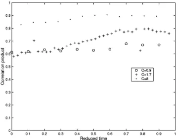
u221v22 1 nbpoints,where (u1,v1) and (u2,v2) are the velocity components given at each point of the PIV mesh grid on two different slices, i and j describe the mesh grid constituted by nbpoints. The correlation product corr is equal to 1 when the ve-locity fields (u1,v1) and (u2,v2) are totally identical. The arithmetical average is computed between the values ob-tained for the upper and middle slices and for the middle and the lower slices. Examples of the correlation product evolu-tion for C50.9, 1.7, and 8 are shown in Fig. 2. The three experiments have different acquisition durations due to the different dynamics which can be more or less propagative. For the cases C50.9, 1.7, and 8 the durations are, respec-tively, 200, 407, and 127 s. In order to compare the evolution of the correlation product on the same graph, the time has been normalized by the acquisition duration. For C50.9, the correlation product increases very slowly from 0.61 to 0.67, the structuration remains weak. For C51.7, the correlation product increases from 0.58 to 0.8 and reach a nearly con-stant value around 0.8. It means that the turbulent patch gen-erated with C51.7 develops progressively in a structured flow on the whole depth. For the most confined case C58, the initial value of the correlation product is greater than 0.8. It increases to reach 0.9 until the end of the acquisition. For
C58 the structuration has occurred before that the flow goes
in the PIV acquisition area.
FIG. 2. Evolution of the correlation product for C50.9 ~symbols s!,
In order to quantify the evolution of the flow structura-tion with respect to the confinement number, we have com-pared the maximum value reached by the correlation product for each experiment. This maximum is called Mcorr. The evolution of Mcorr versus the confinement number C is plot-ted in Fig. 3. We note a direct influence of C on Mcorr while Re has not a significant role. When C is small (C,1), the confinement is too weak to generate a structuration of the flow and the turbulence remains fully three-dimensional ~3D!. From C52, Mcorr remains superior to 0.8, the flow is structured over the depth. The corresponding velocity fields indicate that these structured flows are vortex dipoles. Note that the correlation product never reaches 1. It means that the flow is not perfectly structured, vertical variations remaining even in the most confined experiments. Most of the impul-sive jets generated with C,2 do not develop a structured flow but we have observed episodic emergence of dipoles for
C51.7.
Thus, three regimes can be identified in the jet develop-ment. When C,1, the confinement does not influence the jet, the water layer is deep. A transition occurs when 1,C ,2, where the confinement starts to act on the jet evolution, but the flow is not systematically structured. When C>2, the ‘‘shallow water behavior’’ appears: this is characterized by the flow structuration in large horizontal dipole. We do not have identified any influence of the jet Reynolds number.
V. OBSERVATIONS ON DIPOLES
Vortex dipoles are systematically formed when C>2, and can also appear in the transition zone 1,C,2. The experimental results presented here describe a dipole ob-tained for C53.2 and Re550 000, which features are repre-sentative of all other dipoles we observed in our shallow water experiments.
A. Qualitative observations
Qualitative observations have been carried out by adding fluoresceine or particles in the flow. The pictures shown in Figs. 4 and 5 have been taken for a dipole obtained with C 53.2 and Re550 000.
The particles streaks ~Fig. 4! reveal the main dipole structure with two counter-rotative circulations. The upper
FIG. 3. Maximum of the correlation product versus C for Re550 000 and Re575 000.
FIG. 4. Particle streaks of a dipole obtained with C53.2 and Re550 000 at
t*522.1 ~upper! and t*542 ~lower!.
FIG. 5. Picture of a dipole obtained with C53.2 and Re550 000 at
picture taken at t*522.1 shows the presence of a perturbed
zone in the front of the dipole. This zone is characterized by small-scale turbulent motions. In the latter picture (t*
542), the dipole size has increased. The perturbed zone re-mains in the dipole front, but we also note the presence of 3D turbulent motion in the dipole main flow. A preliminary hypothesis can be done here: 3D small scale turbulence is produced in the frontal region and then transported in the main Q2D dipole flow.
A picture with fluoresceine added to the injected fluid ~Fig. 5! confirms the presence of a perturbed zone in the dipole front. Small scale vortices take place all over the fron-tal boundary.
B. Velocity and vorticity fields
The first quantitative measurements are done on the ve-locity fields. These veve-locity fields are obtained by the PIV system presented in Sec. II.
Figure 6 shows velocity fields and corresponding vortic-ity distributions, respectively, on upper, middle, and lower slices of the dipole obtained with C53.2 and Re550 000. Measurements were done at t*540.3, 40.4, and 40.5. The
shifts correspond to the time necessary to move the light sheet.
The dipolar structure with two counter-rotative circula-tions is easily identified on the velocity fields. The corre-sponding vorticity fields are two patches of opposite sign. However, the dipole structure is not totally identical on the three slices, there is a vertical variation of the flow. The main difference between the velocity fields occurs in the front of the dipole. On the upper slice, the fluid in this frontal zone flows out of the dipole, while on the lower slice the flow clearly comes inside the dipole. In the middle slice, the fron-tal flow is not structured, many small-scale motions are ob-served. These observations reveals the presence of a vertical circulation in the front of the dipole, which is detailed in the following section. Moreover, the flow is not laminar, small shear zones associated to small vortex structures remain in-side the dipole. This feature is confirmed on the vorticity distributions which show numerous patches of various signs. This small-scale turbulence, mainly concentrated in the fron-tal zone, has been previously observed during the qualitative visualizations.
C. Vertical motions
The dipole flow presents a vertical variation in the front of the dipole. The comparison between the velocity fields in the upper and the lower slices suggests the presence of a vertical circulation in the front of the dipole. These observa-tions are confirmed by studying the horizontal divergence of the velocity fields.
The divergence of the velocity field is nil because of the flow incompressibility. Thus, from the horizontal velocity fields, we can compute the gradient of vertical velocity over the vertical direction as follows:
]w/]z52]u/]x2]v/]y.
Figure 7 shows the distribution of]w/]zin the dipole on
the upper and lower slices, respectively, at t*558.2 and at
t*558.4. We note first that the peak value of]w/]z is half the peak value of the vertical vorticity. Then, the horizontal divergence can not be neglected. Even if the main flow takes place in the horizontal plane, the velocity field is not 2D. We note that the distribution of]w/]zis not uniform: the stron-gest vertical velocity gradients are located in the front of the dipole. The comparison between the upper and the lower slices reveals the presence of a vertical circulation. The PIV slices intercept the upper and lower part of this circulation which takes place all along the front of the dipole and all through the depth. The role of this frontal circulation in the production of small-scale turbulence observed in the whole dipole is analyzed in Sec. VI A.
D. vÀc relationship
The Lamb–Chaplygin model of purely 2D dipole as-sumes a linear relationship between the vorticity vand the stream functioncin the dipole. The experiments carried out on dipoles6,10,11 have shown several different relationships betweenvandc. In most cases, thev/crelationship is non-linear and the derivative of the functionv5 f (c) has singu-lar maxima at the vortex cores, but no local maximum else-where.
The stream function is only defined for purely 2D flows. The dipoles observed in shallow water are characterized by significant vertical motion. However, we can assume a scale-separation: A main 2D flow at large length and time scales and 3D turbulent motions at small length and time scales. The main flow is a 2D dipole, which omega–psi relationship can be analyzed. In order to minimize the perturbation due to 3D motions, the vorticity and the stream function are com-puted from the average of the three velocity fields ~on the upper, middle, and lower slices! measured for the case
C53.2 and Re550 000. The so obtained omega–psi relation
is presented in the left part of the Fig. 8. The plot dispersion reveals the presence of small-scale turbulence in the dipole main flow. The small-scale vortices of 3D turbulence provide numerous patches of vorticity which directly induce strong noise in the vorticity signal. The stream function which is defined from two successive spatial integrations of the vor-ticity is less affected by the presence of small scale motion. In order to evaluate the omega–psi relationship of the 2D main flow and to avoid perturbations due to small-scale tur-bulence, we have averaged the vorticity values obtained for each stream function calculation. The result is plotted on the right part of the Fig. 8. It allows to identify the nonlinear relationship between the vorticity and the stream function of the dipole main flow. The shape of the omega–psi relation is different from the sinh-relation observed in stratified or mag-netically driven flows. We can note that the two branches
v.0 and v,0 which each represent one half of the dipole are more spaced than in a sinh-relation. It means that the two vortices are less linked and are separated by a nearly irrota-tional flow. It reveals an increase of fluid entrainment, prob-ably caused by the vertical circulation at the dipole front. This observation can also be relied to the numerical simula-tions of dipole in stratified fluid carried out by Beckers
et al.19For the higher Reynolds number simulations, dipoles ~which remain laminar! are found to be less compact, with a kink in the vorticity profile. For increasing Reynolds number, entrainment of nearly irrotational fluid into the dipole comes more effective in forming less compact dipoles, be-cause diffusion is less effective in smoothing the vorticity profile. Such a mechanism can explain the appearance of a
kink in the vorticity profile in our turbulent dipole experi-ments.
E. Summary of the observations
The present experiments have highlighted the main fea-tures of dipoles in a shallow water layer. These dipoles are
FIG. 6. Dipole velocity field ~left! and vorticity field ~right! for C53.2 and Re550 000: upper figure at t*540.3 on the upper slice, middle figure at t*
quite different from their counterparts observed in Q2D flows. Firstly, the dipoles are turbulent: 3D turbulence is ad-vected by the Q2D main flow. These small scale perturba-tions are responsible for the dispersion of the v/c relation-ship. Secondly, vertical motion remains significant during the dipole evolution. These motion are mainly concentrated in a vertical circulation which takes place in the dipole front all over the depth.
VI. THEORETICAL MODEL A. Hypothesis
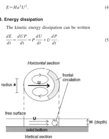
We have used the previous observations to model the dipole evolution and to understand the presence of small-scale turbulence in the main flow. Our model aims at describ-ing the evolution of a dipole in linear translation, of speed U and radius a with a vertical circulation in the frontal zone ~Fig. 9!.
The equilibrium of the boundary layer corresponds to the balance between the diffusion and advection times of the momentum. This leads to
d2
v ' H U.
Then, the boundary layer thicknessd can be estimated
d'
A
v H U.By considering the characteristic values U50.02 m/s,
v51026m2• s21 and H50.3 m, the boundary layer
Rey-nolds number Redis about 80, which is far from the critical
value Red5300. Then, the boundary layer is considered
stable. We assume that the frontal circulation of the dipole is the only responsible of small-scale turbulence production.
The momentum P ~divided byr! and the kinetic energy
E ~divided byr! are, respectively, evaluated by
P'Ha2U
, ~3!
E'Ha2U2
. ~4!
B. Energy dissipation
The kinetic energy dissipation can be written
dE dt 5 dU P dt 5 P dU dt 1U d P dt . ~5!
FIG. 7. Horizontal divergence field ~left for upper slice and right for lower slice, units s21!, at t*
558.2 and t*558.4, C53.2 and Re550 000 ~the black arrow
represents the jet axis!.
FIG. 8. Vorticity/stream-function relationship for C53.2, Re550 000 and
t*558.3, direct computation ~left figure! and averaged vorticity
1. Estimation of P(dUÕdt)
This term is associated to the turbulence production which occurs in the frontal circulation, characterized by its thickness H and its ‘‘active’’ volume aH2. The energy dissi-pation rate in the circulation can be written as the product of the volumic dissipation U3/H by the active volume
PdU dt '2 U3 H aH 2 '2U3aH '2EUa . ~6!
The radius a can be expressed from Eq. ~3!: a ' P1/2U21/2H21/2. Then Eq. ~6! becomes
PdU dt '2U
5/2P1/2H1/2
. ~7!
2. Estimation of U(dPÕdt)
This term is nil if the momentum is constant. A remark-able property of the 2D dipoles is to transport momentum as a solid body does. Significant vertical motions have been observed in the shallow water dipoles. It is of great interest to know how these long-lifetime vortices are able to trans-port momentum.
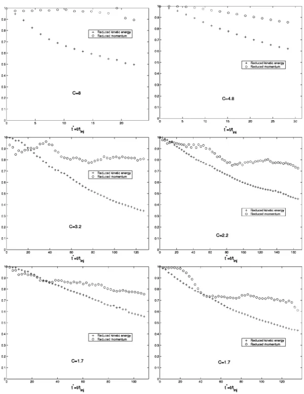
FIG. 10. Evolution of reduced momentum and reduced kinetic energy. For C58 ~Re550 000!, C54.8 ~Re550 000!, C53.2 ~Re550 000!, C52.2 ~Re550 000!, C51.7 ~Re575 000!, and C51.7 ~Re550 000!.
If P is not constant, its dissipation is mainly caused by the bottom friction. It can be estimated by
d P dt 'v
E
]v ]z dr 2 . ~8!The shear ]v/]z can be approximated by U/d, where d is
the boundary layer thickness. Equation ~8! becomes
d P dt 'v
Ua2
d . ~9!
Then Eq. ~9! can be written
d P dt '2v 1/2U3/2H21/2a2, ~10! which leads to Ud P dt '2v 1/2U5/2H21/2a2 . ~11!
3. Comparison of both contributions
From Eqs. ~6! and ~11!, the total kinetic energy dissipa-tion becomes dE dt '2U 3 aH2v1/2U5/2H21/2a2 . ~12!
The contributions of both terms can be evaluated by computing their ratio
PdU dt Ud P dt 5U3aHv21/2U25/2H1/2a225U1/2H3/2a21v21/2. ~13! If we introduce the parametrization of shallow water flows proposed by Dolzhanskii et al.,20 two different Rey-nolds numbers can be defined. On one hand, the internal Reynolds number characterizes the horizontal structure
Rea5Ua
v . ~14!
On the other hand, the external Reynolds number takes into account the bottom friction
Ref5lLU 5UH 2
2av , ~15!
where L is the characteristic horizontal lengthscale and l is the bottom friction coefficient given by l52v/H2for a thin fluid layer.
Equation ~13! can be written
PdU dt Ud P dt 5
S
UH 2 2avD
3/4S
Ua vD
21/4 ~16! 5S
Ref 3 ReaD
1/4 . ~17!Two different regimes are possible: ~i! If (Ref
3
/Rea)1/4.1 (Ref3@Rea), the term PdU/dt domi-nates, the frontal circulation has a preponderant influ-ence, the momentum dissipation can be neglected. ~ii! If (Ref
3
/Rea)1/4,1 (Ref3,Rea), the momentum cannot be considered constant. This regime has been characterized in the parametrization of bottom friction in the shallow water equations, see for instance, Ref. 21.
C. Velocity and radius evolution
In the case where (Ref 3
/Rea)1/4.1, the momentum is considered constant. Then evolution laws for U and a can be deduced from expression ~7!
U'
S
P HD
1/3 ~ t2t0!22/3, a'S
P HD
1/3 ~ t2t0!1/3. ~18! This time dependence of the dipole radius is similar to the one obtained in the experiments carried out on dipoles in stratified fluid by Voropayev et al.7VII. COMPARISON WITH EXPERIMENTAL RESULTS A. Momentum measurements
The first step of the model validation is to quantify the momentum evolution during the dipole translation and to compare it with the kinetic energy evolution.
Six nearly symmetric dipoles in linear translation have been studied. From the three horizontal slices, the velocity fields (u,v) are obtained all along the dipole evolution. The momentum Pi and the kinetic energy Ei ~divided byr! are computed on the slice ~i! as follows:
Pi5
A
S
(
S udSD
2 1S
(
S vdSD
2 , Ei51/2(
S ~ u2 1v2!dS,where S is the PIV meshgrid surface and dS the surface element. The average values P and E are computed between the three slices. By dividing P and E by their respective maxima, the reduced momentum P* and the reduced kinetic energy E* are obtained.
Figure 10 shows the compared evolutions of P*and E*
for six different dipoles, respectively, represented by
sym-TABLE I. (Ref
3
/Rea)
1/4
versus C and Re.
C Reinj (Ref
3
/Rea)1/4initial (Ref
3
/Rea)1/4final Final time ~s!
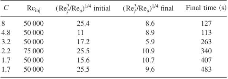
8 50 000 25.4 8.6 127 4.8 50 000 11 8.9 113 3.2 50 000 17.2 5.9 263 2.2 75 000 25.5 10.9 340 1.7 50 000 15.6 10.7 407 1.7 50 000 25.5 9.6 483
bols s and 1. The dimensionless time is defined by
t*5t/tinj. The initial time t*50 is the beginning of the PIV acquisition.
We first note that, in all cases, the reduced momentum is better conserved than reduced kinetic energy. However, the momentum dissipation is never negligible. This dissipation is weak in the most confined case (C58 in Fig. 10! but re-mains significant. Thus, we have shown that, during the propagation of dipoles in shallow water, the momentum is not strictly conserved. The momentum dissipation is associ-ated to the bottom friction, which contribution in the kinetic energy dissipation is evaluated by the term U(d P/dt) in Eq. ~5!.
As shown previously, the contributions of both terms
U(d P/dt) and P(dU/dt) in the kinetic energy dissipation can be evaluated by the ratio (Ref
3
/Rea)1/4. We compute the values of Ref, Rea and (Ref
3
/Rea)1/4 for each dipole, at the initial and final time of the acquisition. The characteristic speed U is determined on the dipole axis and the radius a is defined as the distance between the vorticity extrema. These calculations are exposed in the Table I.
Two observations can be done from these results: ~i! (Ref
3
/Rea)1/4 is systematically greater than 1. It means that the term P(dU/dt) dominates U(d P/dt) in Eq. ~17!. In first approximation, we can neglect the term FIG. 11. Evolution of reduced velocity on upper slice ~symbols*!, middle slice ~symbols 1!, and lower slice ~symbols s!, and comparison with theoretical model U*5A(t*2t0*)22/3~solid line!.
U(d P/dt) in the kinetic energy dissipation, which cor-responds to considering the momentum constant during the dipole evolution.
~ii! (Ref 3
/Rea)1/4 decreases during time. The regime consid-ered here, where the momentum dissipation is neglected and the turbulence production in the frontal circulation is the main responsible of kinetic energy dissipation, will progressively degenerate in a different regime where both contributions are of the same order.
The assumption P5cste allows to write evolution laws for the characteristic velocity and radius in Eq. ~18!.
B. Model validation
In order to validate our model, its predictions are com-pared with the experimental results for the dipole velocity and radius. The evolution laws are given by
U'A~ t2t0!22/3, a'B~ t2t0!1/3, ~19! where A and B are constant and t0is, respectively, defined by
U(t0)5U0 where U0 is the initial dipole velocity and
a(t0)5a0 where a0 is the initial dipole radius. The reduced velocity U* and the reduced radius a* are obtained by di-viding the measured values U and a by the initial values:
U*5U/U0 and a*5a/a0.
1. Evolution of characteristic velocity
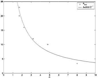
Figure 11 presents the evolutions of the characteristic velocity measured on the three slices compared to the model prediction. In every case, we can note a good agreement between the model prediction and the experimental results. The constant A takes respectively the following values: 3.4, 10, 12, 16, 23, and 20. In Fig. 12, the experimental values
Aexpare plotted versus C and compared to a hyperbolic evo-lution A536.8C21. The reduced characteristic velocity of turbulent shallow water dipoles can be expressed as follows:
U*536.8C21~ t*2t0*!22/3. ~20!
2. Evolution of radius
The dipole radius is computed from the vorticity field obtained from the PIV velocity field. By identifying at each instant the vorticity extrema positions, we deduce the dis-tance between the circulation centers, called a.
Figure 13 presents the evolutions of the reduced radius measured on the three slices compared to the model predic-tion. The constant B takes, respectively, the values: 0.6, 0.2, 0.1, 0.2, 0.2, and 0.05.
The model predictions for the dipole radius are less ac-curate than for the velocity evolution. The dipole radius, identified as the distance between the circulation centers, does not increase systematically. In the cases C54.8 and C 51.7, it tends to decrease during time. If we compare the vorticity distribution obtained at t*525.6 and t*5131.5 in
the last case (C51.7) in Fig. 14, we observe that the circu-lation centers get closer during time while the dipole lateral extension increases mainly by lateral diffusion. Unfortu-nately, the total dipole lateral extension cannot be correctly measured because of the difficulty to define a boundary to the dipole flow.
We can also observe an oscillation of the dipole radius around its evolution. These oscillations are not identical on the three slices, there is a phase shift. The vorticity axes do not remain parallel during time. Dipoles are submitted to horizontal oscillations, which lead to conical shapes alterna-tively oriented downward and upward. This phenomenon is less evident in the most confined case C58.
VIII. CONCLUSION
Laboratory experiments aimed at studying the vortex dy-namics generated by impulsive jets have been performed in shallow water layer. Our aim was to identify a transition from fully 3D behavior ~deep fluid layer! to Q2D behavior ~shallow water layer!. This transition has been studied by imposing a progressive vertical confinement on an axisym-metric horizontal turbulent impulsive jet. The jet evolution has been studied depending on two dimensionless param-eters: the Reynolds number Re and the confinement number
C. They are defined by
Re5
A
vQ, C5A
Q H2 tinj,where v is the kinematic viscosity, Q the injected momentum flux, H the water depth and tinj the injection duration. The development of horizontal impulsive jets is only controlled by the confinement number C whereas the Reynolds number has no influence in the studied range. When C is inferior to 1, the impulsive jet development is a typical three-dimensional turbulence decay, the water layer is deep. Between C51 and
C52, the confinement starts to act on the flow, vertical
mo-tions are progressively damped. Beyond C52, the impulsive jet develops into vortex dipole, which size is much larger than the fluid depth, the water layer can be considered shal-low.
A detailed study of turbulent dipoles in shallow water layer have been carried out. The velocity and vorticity fields show the relative homogeneity of the dipoles over the depth FIG. 12. Evolution of the constant A versus the confinement number C
and the quasi-two-dimensionality of the main flow. However, the dipoles are turbulent: 3D turbulent motions are trans-ported by the Q2D main flow. Observations have revealed the presence of a vertical circulation in the dipole front. The boundary layer on the solid bottom is stable and the frontal circulation is the only responsible of small-scale turbulence production. The contributions of bottom friction and frontal circulation in the kinetic energy dissipation are controlled by the ratio (Ref
3 /Rea)
1/4
(Rea5Ua/v and Ref5UH2/2av where
Uis the characteristic velocity and a the dipole radius!. Mea-surements have shown that (Ref
3
/Rea)1/4is greater than 1 for every dipole observed in shallow water. Thus, even if the momentum is not strictly conserved, the effects of momen-tum dissipation by bottom friction can be neglected. Two
evolution laws for the velocity U and radius a of the dipoles can be deduced from the model: U5A(t2t0)22/3where t0is defined by U(t0)5U0 with U0 the initial speed and A is a constant, and a5B(t2t0)1/3 where B is a constant and
a(t0)5a0 where a0is the dipole initial radius. The compari-son with experimental results shows a good agreement for the velocity evolution. Such comparison is more difficult for the radius evolution because of the difficulty to carry out accurate measurements.
Thus, we have characterized the conditions necessary to the formation of dipoles in a shallow water layer and detailed the flow structure. However, these experimental results lead us to several questions, in particular the role of the solid bottom in the formation of a vertical circulation in the dipole
FIG. 13. Evolution of reduced radius on upper slice ~symbols*!, middle slice ~symbols 1!, and lower slice ~symbols s!, and comparison with theoretical
model a5B(t*2t0*) 1/3
front. Preliminary qualitative observations have been carried out at small scale on laminar dipoles with a slip condition on the bottom ~addition of a heavier fluid layer!. These obser-vations have revealed the quasi-two-dimensional structure of the flow, without vertical circulation at the dipole front.22
ACKNOWLEDGMENTS
The present experiments have been performed on the Coriolis turntable of the LEGI ~Grenoble! and thanks to the financial support of the De´le´gation Ge´ne´rale pour l’Armement.
1H. Lamb, Hydrodynamics, 6th ed. ~Dover, New York, 1932!.
2V. V. Meleshko and G. J. F. Van Heijst, ‘‘On Chaplygin’s investigations of
two-dimensional vortex structures in an inviscid fluid,’’ J. Fluid Mech.
272, 157 ~1994!.
3J. C. McWilliams, ‘‘The vortices of two-dimensional turbulence,’’ J. Fluid
Mech. 219, 361 ~1990!.
4J. A. Smith and J. L. Largier, ‘‘Observations of nearshore circulations: Rip
currents,’’ J. Geophys. Res. 100, 10967 ~1995!.
5
T. Fujiwara, H. Nakata, and K. Nakatsuji, ‘‘Tidal-jet and vortex-pair driv-ing of the residual circulation in a tidal estuary,’’ Cont. Shelf Res. 14, 1025 ~1994!.
6J. B. Flo`r and G. J. F. Van Heijst, ‘‘An experimental study of dipolar
vortex structures in a stratified fluid,’’ J. Fluid Mech. 279, 101 ~1994!.
7S. I. Voropayev, Ya. D. Afanasyev, and I. A. Filippov, ‘‘Horizontal jets and
vortex dipoles in a stratified fluid,’’ J. Fluid Mech. 227, 543 ~1991!.
8D. C. Montgomery and G. Joyce, ‘‘Statistical mechanics of ‘negative
tem-perature’ states,’’ Phys. Fluids 17, 1139 ~1974!.
9E. J. Hopfinger and G. J. F. Van Heijst, ‘‘Vortices in rotating fluids,’’ J.
Fluid Mech. 25, 241 ~1993!.
10O. U. Velasco Fuentes and G. J. F. Van Heijst, ‘‘Experimental study of
dipolar vortices on a topographicb-plane,’’ J. Fluid Mech. 259, 79 ~1994!.
11J. M. Nguyen Duc and J. Sommeria, ‘‘Experimental characterization of
steady two-dimensional vortex couples,’’ J. Fluid Mech. 192, 175 ~1988!.
12Y. Couder and C. Basdevant, ‘‘Experimental and numerical study of
vor-tex couples in two-dimensional flows,’’ J. Fluid Mech. 173, 225 ~1986!.
13W. S. J. Uijttewaal and R. Booij, ‘‘Effects of shallowness on the
develop-ment of free-surface mixing layers,’’ Phys. Fluids 12, 392 ~2000!.
14
R. Booij and J. Tukker, ‘‘Integral model of shallow mixing layers,’’ J. Hydraul. Res. 39, 169 ~2001!.
15
W. S. J. Uijttewaal and G. H. Jirka, ‘‘Grid turbulence in shallow flows,’’ J. Fluid Mech. 489, 325 ~2003!.
16A. M. Fincham and G. R. Spedding, ‘‘Low cost, high resolution DPIV for
measurement of turbulent fluid flow,’’ Exp. Fluids 23, 449 ~1997!.
17A. Fincham and G. Delerce, ‘‘Advanced optimization of correlation
imag-ing velocimetry algorithms,’’ Exp. Fluids 29, S13 ~2000!.
18H. Schlichting, Boundary Layer Theory ~McGraw-Hill, New York, 1979!. 19
M. Beckers, H. J. H. Clercx, G. J. F. Van Heijst, and R. Verzicco, ‘‘Dipole formation by two interacting shielded monopoles in a stratified fluid,’’ Phys. Fluids 14, 704 ~2002!.
20F. V. Dolzhanskii, V. A. Krymov, and D. Yu. Manin, ‘‘An advanced
ex-perimental investigation of quasi-two-dimensionnal shear flows,’’ J. Fluid Mech. 241, 705 ~1992!.
21H. J. H. Clercx, G. J. F. Van Heijst, and M. L. Zoeteweij,
‘‘Quasi-two-dimensional turbulence in shallow fluid layers: The role of bottom friction and fluid layer depth,’’ Phys. Rev. E 67, 066303 ~2003!.
22D. Sous, ‘‘Dynamique tourbillonnaire en milieu peu profond,’’ Ph.D.
the-sis, Universite´ Bordeaux 1 ~2003!.