HAL Id: hal-00296471
https://hal.archives-ouvertes.fr/hal-00296471
Submitted on 4 Mar 2008
HAL is a multi-disciplinary open access
archive for the deposit and dissemination of
sci-entific research documents, whether they are
pub-lished or not. The documents may come from
teaching and research institutions in France or
abroad, or from public or private research centers.
L’archive ouverte pluridisciplinaire HAL, est
destinée au dépôt et à la diffusion de documents
scientifiques de niveau recherche, publiés ou non,
émanant des établissements d’enseignement et de
recherche français ou étrangers, des laboratoires
publics ou privés.
CALIPSO cloud height and amount
B. H. Kahn, M. T. Chahine, G. L. Stephens, G. G. Mace, R. T. Marchand, Z.
Wang, C. D. Barnet, A. Eldering, R. E. Holz, R. E. Kuehn, et al.
To cite this version:
B. H. Kahn, M. T. Chahine, G. L. Stephens, G. G. Mace, R. T. Marchand, et al.. Cloud type
comparisons of AIRS, CloudSat, and CALIPSO cloud height and amount. Atmospheric Chemistry
and Physics, European Geosciences Union, 2008, 8 (5), pp.1231-1248. �hal-00296471�
www.atmos-chem-phys.net/8/1231/2008/ © Author(s) 2008. This work is distributed under the Creative Commons Attribution 3.0 License.
Chemistry
and Physics
Cloud type comparisons of AIRS, CloudSat, and CALIPSO cloud
height and amount
B. H. Kahn1, M. T. Chahine1, G. L. Stephens2, G. G. Mace3, R. T. Marchand4, Z. Wang5, C. D. Barnet6, A. Eldering1,
R. E. Holz7, R. E. Kuehn8, and D. G. Vane1
1Jet Propulsion Laboratory, California Institute of Technology, Pasadena, CA, USA 2Department of Atmospheric Science, Colorado State University, Fort Collins, CO, USA 3Department of Meteorology, University of Utah, Salt Lake City, UT, USA
4Joint Institute for the Study of the Atmosphere and Ocean, University of Washington, Seattle, WA, USA 5Department of Atmospheric Science, University of Wyoming, Laramie, WY, USA
6NOAA – NESDIS, Silver Springs, MD, USA
7CIMSS – University of Wisconsin – Madison, Madison, WI, USA 8NASA Langley Research Center, Hampton, VA, USA
Received: 14 September 2007 – Published in Atmos. Chem. Phys. Discuss.: 27 September 2007 Revised: 20 December 2007 – Accepted: 5 February 2008 – Published: 4 March 2008
Abstract. The precision of the two-layer cloud height fields derived from the Atmospheric Infrared Sounder (AIRS) is explored and quantified for a five-day set of observations. Coincident profiles of vertical cloud structure by CloudSat, a 94 GHz profiling radar, and the Cloud-Aerosol Lidar and In-frared Pathfinder Satellite Observation (CALIPSO), are com-pared to AIRS for a wide range of cloud types. Bias and variability in cloud height differences are shown to have dependence on cloud type, height, and amount, as well as whether CloudSat or CALIPSO is used as the comparison standard. The CloudSat-AIRS biases and variability range from −4.3 to 0.5±1.2–3.6 km for all cloud types. Likewise, the CALIPSO-AIRS biases range from 0.6–3.0±1.2–3.6 km (−5.8 to −0.2±0.5–2.7 km) for clouds ≥7 km (<7 km). The upper layer of AIRS has the greatest sensitivity to Altocumu-lus, Altostratus, Cirrus, Cumulonimbus, and Nimbostratus, whereas the lower layer has the greatest sensitivity to Cu-mulus and StratocuCu-mulus. Although the bias and variability generally decrease with increasing cloud amount, the ability of AIRS to constrain cloud occurrence, height, and amount is demonstrated across all cloud types for many geophysi-cal conditions. In particular, skill is demonstrated for thin
Correspondence to: B. H. Kahn ([email protected])
Cirrus, as well as some Cumulus and Stratocumulus, cloud types infrared sounders typically struggle to quantify. Fur-thermore, some improvements in the AIRS Version 5 opera-tional retrieval algorithm are demonstrated. However, limi-tations in AIRS cloud retrievals are also revealed, including the existence of spurious Cirrus near the tropopause and low cloud layers within Cumulonimbus and Nimbostratus clouds. Likely causes of spurious clouds are identified and the poten-tial for further improvement is discussed.
1 Introduction
Improving the realism of cloud fields within general circu-lation models (GCMs) is necessary to increase certainty in prognoses of future climate (Houghton et al., 2001). How-ever, cloud responses to anthropogenic forcing in climate GCMs vary widely from model to model and are largely at-tributed to differences in the representation of cloud feed-back processes (Stephens, 2005). Use of relatively long-term satellite data records such as the Earth Radiation Bud-get Experiment (ERBE) (Ramanathan et al., 1989) and the International Satellite Cloud Climatology Project (ISCCP) (Rossow and Schiffer, 1999) have clarified cloud radiative impacts, inspired approaches to climate GCM evaluation, and contributed to further theoretical understanding of cloud
feedbacks (e.g. Hartmann et al., 2001). Wielicki et al. (1995) note the historical satellite record is unable to measure all cloud properties relevant to Earth’s cloudy radiation budget, which include liquid and ice water path (LWP/IWP), visible optical depth (τ ), effective particle size (De), particle phase
and shape, fractional coverage, height, and IR emittance. Il-lustrating the need for improved cloud observations, Webb et al. (2001) showed that some climate GCMs generate erro-neous vertical cloud distributions that compensate in a man-ner producing favorable mean radiative budget comparisons with observations. Thus, reliable observations of cloud ver-tical structure will help to reduce the ambiguity in climate GCM–satellite comparisons.
Several active and passive satellite sensors with unprece-dented observing capabilities are flying in a formation called the “A-train” (Stephens et al., 2002). The constellation is anchored by NASA’s Earth Observing System (EOS) Aqua and Aura satellites, the Cloud-Aerosol Lidar and Infrared Pathfinder Satellite Observation (CALIPSO) (Winker et al., 2003), CloudSat (Stephens et al., 2002), along with the Polar-ization and Anisotropy of Reflectances for Atmospheric Sci-ences coupled with Observations from a Lidar (PARASOL), and in the near future Glory (solar irradiance and aerosols), and the Orbiting Carbon Observatory (OCO) (atmospheric CO2). Several instruments on Aqua and Aura are designed to
measure temperature, humidity, clouds, aerosols, trace gases, and surface properties (Parkinson et al., 2003; Schoeberl et al., 2006). The present focus is on comparisons of cloud retrievals from the Atmospheric Infrared Sounder (AIRS) lo-cated on Aqua (Aumann et al., 2003) to CloudSat, a 94 GHz cloud profiling radar, and CALIOP (Cloud-Aerosol Lidar with Orthogonal Polarization), a cloud and aerosol profiling lidar on CALIPSO. Aqua leads CloudSat and CALIPSO by
∼55 and ∼70 s, respectively, providing nearly simultaneous and collocated cloud observations.
From the perspective of a satellite-based cloud observa-tion, inter-satellite comparisons have several advantages over surface-satellite comparisons: they (1) eliminate the ambigu-ity introduced from the integration of a time series of surface-based measurements to replicate a spatial scale comparable to the satellite field of view (FOV) that is further complicated by cloud temporal evolution (e.g. Kahn et al., 2005), (2) re-duce the effects of certain types of sampling biases, includ-ing those introduced by the attenuation of surface-based lidar and cloud radar in thick and precipitating clouds (Comstock et al., 2002; McGill et al., 2004), (3) provide a larger and sta-tistically robust set of observations for comparison, and (4) facilitate near-global sampling for most types of clouds.
Many schemes have been developed to classify clouds into fixed types. For instance, the ISCCP data set provides a 3×3 classification scheme based on cloud top pressure and
τVIS (Rossow and Schiffer, 1999), while Wang and Sassen
(2001) developed a scheme using multiple ground-based sen-sors. These (and numerous other) classification schemes are loosely based on the naming system originating from Luke
Howard (Gedzelman, 1989). Although cloud classification schemes are limited by measurement sensitivity and subject to misinterpretation, they help to organize clouds into cate-gories with unique characteristics of composition, radiative forcing, and heating/cooling effects (Hartmann et al., 1992; Klein and Hartmann, 1993; Chen et al., 2000; Inoue and Ackerman, 2002; Xu et al., 2005; L’Ecuyer et al., 2006).
No single passive or active measurement from space is able to infer all relevant cloud physical properties (e.g. Wielicki et al., 1995) spanning all geophysical conditions; hence, a multi-instrument constellation is needed to observe Earth’s clouds (Miller et al., 2000; Stephens et al., 2002). Now that this type of satellite constellation is operational, the strengths and weaknesses of various instruments can be evaluated in the presence of different cloud types and ul-timately observations of multiple instruments can be com-bined to yield retrievals superior to retrievals from any single instrument. This is motivated in part because of discrepan-cies in existing climatologies of cloud height, frequency and amount derived from combinations of passive (visible, IR, and microwave) wavelengths (e.g. Rossow et al., 1993; Jin et al., 1996; Thomas et al., 2004). Discrepancies exist not only from different measurement characteristics and sam-pling strategies, but perhaps as significantly, from retrieval algorithm differences and a priori assumptions (Rossow et al., 1985; Wielicki and Parker, 1992; Kahn et al., 2007b). CloudSat and CALIOP generally provide more direct and easily interpreted observations of cloud detection and vertical cloud structure than passive methods. A combination of ra-diative transfer modeling and a priori assumptions of surface and atmospheric quantities are necessary to infer cloud prop-erties from passive measurements (e.g. Rossow and Schiffer, 1999).
The scientific literature is replete with cross-comparisons of in situ, surface-based, and satellite-derived cloud proper-ties. However, there are few that consider the impacts of cloud type on the distribution of statistical properties. The precision of passive satellite-derived cloud quantities is not only impacted by cloud type, but temperature (Susskind et al., 2006) and water vapor variability (Fetzer et al., 2006), trace gases (Kulawik et al., 2006), aerosols (Remer et al., 2005), and surface quantities have varying degrees of preci-sion within different cloud types. In this article, the accuracy of AIRS cloud height and amount for different cloud type configurations is quantified using CloudSat and CALIPSO. In Sect. 2 the observations and data products of the three observing platforms are introduced. Section 3 describes the comparison methodology and presents illustrative cloud climatologies of AIRS, CloudSat, and CALIOP. Similari-ties and differences are placed in the context of measure-ment sensitivity. Section 4 presents coincident CloudSat-AIRS cloud top differences spanning the breadth of cloud types. CALIPSO-AIRS cloud top differences are shown and compared to those between CloudSat-AIRS. Further-more, strengths and weaknesses of AIRS cloud retrievals are
revealed and probable causes of discrepancies are discussed. In Sect. 5 the results are discussed and summarized.
2 Data
The sensitivity of radar, lidar and passive IR sounders to clouds differs greatly. Active sensors provide relatively di-rect observations of cloud vertical structure compared to pas-sive IR sounders, which derive cloud vertical structure using combinations of radiative transfer modeling and a priori as-sumptions about the surface and atmospheric state. AIRS has sensitivity to clouds with τVIS≤10 (Huang et al., 2004).
CALIOP can be used to obtain very accurate cloud top boundaries, especially when the cloud scatters visible light well above that of the molecular atmosphere and aerosols, but has an upper bound of τVIS∼3 (Winker et al., 1998; You
et al., 2006). CloudSat penetrates through clouds well be-yond the sensitivity limit of IR sounders, but is insensitive to small hydrometeors and will often miss tenuous cloud con-densate at the tops of some clouds or clouds composed only of small liquid water droplets. In this comparison, a subset of publicly released products is used: cloud top height (ZA)
and effective cloud fraction (fA)from AIRS, the radar-only
cloud confidence and cloud classification masks from Cloud-Sat, and the 5 km cloud feature mask from CALIPSO.
2.1 AIRS
AIRS is a thermal IR grating spectrometer operating in tan-dem with the Advanced Microwave Sounding Unit (AMSU) (Aumann et al., 2003). A substantial portion of Earth’s ther-mal emission spectrum is observed with 2378 spectral chan-nels from 3.7–15.4 µm at a nominal spectral resolution of
υ/1υ≈1200. The AIRS footprint size is 13.5 km at nadir, whereas AMSU is approximately 40 km at nadir and co-aligned to a 3×3 array of AIRS FOVs. The AIRS/AMSU suite scans ±48.95◦ off nadir recording over 2.9 million AIRS spectra and 300 000 Level 2 (L2) retrievals for daily, near-global coverage. The Version 5 (V5) AIRS L2 oper-ational retrieval system (and all previous versions) is based on the cloud-clearing approach of Chahine (1974). Unless otherwise noted the AIRS retrievals used are V5. Profiles of
T (z), q(z), O3(z), additional minor gases such as CH4, CO,
CO2and SO2, and other atmospheric and surface properties
are derived from the cloud-cleared radiances (Chahine et al., 2006).
Up to two cloud layers are inferred from fitting observed AIRS radiances to calculated ones (Kahn et al., 2007a). Cloud top pressure (PA)and cloud top temperature (TA)are
reported at the AMSU resolution (∼40 km at nadir), whereas
fA – the multiplication of spatial cloud fraction and cloud
emissivity – is reported at the AIRS resolution. (Henceforth, “AIRS FOV” refers to the spatial scale of geophysical param-eters reported at the AMSU FOV resolution unless otherwise
noted.) ZA is derived from PA and geopotential height
us-ing a log-linear interpolation of PAin between adjacent
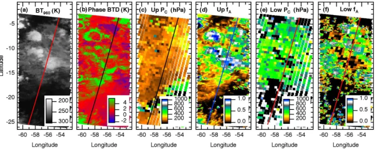
stan-dard geopotential levels. An illustrative (and partial) AIRS granule (defined to be 135 scan lines or 6 min of data) is pre-sented in Fig. 1. Shown is the brightness temperature (BT) at 960 cm−1 (BT960), a BT difference between 1231 cm−1
and 960 cm−1(BTD) that reveals a sensitivity to cloud phase (Nasiri et al., 2007), and PA and fA for two cloud layers.
A wide variety of structure, including extensive multi-layer clouds, is observed in the PA and fAfields. Figure 1b
indi-cates negative BTDs from 6–8◦S that coincide with Altocu-mulus (Ac) and Altostratus (As) and higher values of PAand
fA, whereas scattered positive BTD are present to the north
and south within thinner Cirrus (Ci) layers having lower val-ues of PAand fA. The negative and positive BTDs coincide
with cloud types consistent with liquid water droplets (Ac and As) and ice crystals (Ci), respectively (see Sect. 2.2). For further detail about AIRS cloud retrievals, cloud valida-tion efforts, and cross-comparisons with the Moderate Reso-lution Imaging Spectroradiometer (MODIS) and Microwave Limb Sounder (MLS), please refer to Susskind et al. (2006), Kahn et al. (2007a, b), Weisz et al. (2007), and references therein.
2.2 CloudSat
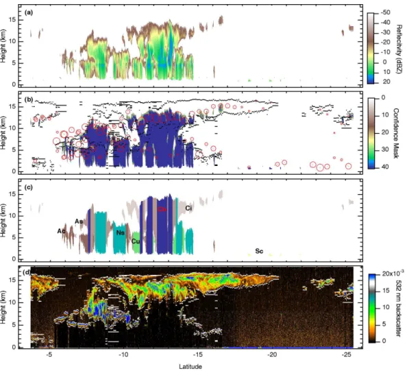
CloudSat is a 94 GHz cloud profiling radar providing vertically-resolved information on cloud location, cloud ice and liquid water content (IWC/LWC), precipitation, cloud classification, radiative fluxes and heating rates (Stephens et al., 2002). The vertical resolution is 480 m with 240 m sam-pling, and the horizontal resolution is approximately 1.4 km (cross-track) ×2.5 km (along-track) with sampling roughly every 1 km. Surface reflection/clutter over most surfaces greatly reduces radar sensitivity in the lowest 3–4 range bins (roughly the lowest km) such that these data are marginally useful in release 3 (R03) (Marchand et al., 2008). An ex-ample cross-section of height-resolved reflectivity is shown in Fig. 2a for the same granule introduced in Fig. 1. Cloud-Sat reveals details in vertical cloud structure that IR sounders are unable to either resolve or sample because the IR signal is emitted by the upper 8–10 or so optical depths of a given cloud profile (Huang et al., 2004).
Range bins with detectable hydrometeors are reported in the 2B-GEOPROF product (Mace et al., 2007). A cloudy range bin is associated with a confidence mask value that ranges from 0–40. Values ≥30 are confidently associated with clouds although values as low as 6 suggest clouds ap-proximately 50% of the time (Marchand et al., 2008). Fig-ure 2b shows the cloud mask for confidence values ≥20. When compared to AIRS cloud fields (Figs. 1 and 2b), PA
agrees better with CloudSat when fAis relatively large. In
more tenuous scenes (small fA)CloudSat infrequently
ob-serves clouds. It is unclear if this is a result of clouds with low radar reflectivities (due perhaps to small hydrometeor
Fig. 1. An illustrative AIRS granule (number 53) from a descending orbit on 26 October 2006 (05:12:00–05:18:00 UTC). (a) AIRS BT at
960 cm−1. (b) AIRS BT difference (1231–960 cm−1)indicating cloud phase sensitivity. (c) AIRS upper cloud top pressure (PC)(hPa). (d)
AIRS effective cloud fraction (fA)associated with the upper PC. (e) As in (c) except for the lower PC. (f) As in (d) except for the lower
layer fA. Lines with various colors indicate the CloudSat ground track that trails the AIRS observation by approximately 55 s.
size), or spurious AIRS cloud retrievals, or just simple mis-matches in the sensor time and space sampling. This sub-ject is discussed in Sects. 3 and 4. About 51% of all R03 CloudSat profiles confidently contain at least one range bin with hydrometeors based on three months of data from the Summer of 2006 (Mace et al., 2007). In Release 4 (R04), a combined radar-lidar 2B-GEOPROF product will be pro-duced (Marchand et al., 2008).
The detected clouds in 2B-GEOPROF are assigned cloud types and are reported in the 2B-CLDCLASS product (Wang and Sassen 2007). Clouds with a confidence mask ≥20 are classified into Ac, As, Cumulonimbus (Cb), Ci, Cumulus (Cu), Nimbostratus (Ns), Stratocumulus (Sc), and Stratus (St). The two-dimensional structure and maximum value of cloud reflectivity as well as cloud temperature (based on ECMWF profiles) are combined to identify cloud types. Cloud type frequency and spatial statistics are presented in Wang and Sassen (2007) for the initial 6 months of CloudSat observations. In a future version a radar-lidar cloud classi-fication mask will be released. The radar-only cloud clas-sification scheme has some differences when compared to a combined radar-lidar scheme. The cloud types As, Ns, Cb, and Cu (congestus) are well detected and classified with a radar-only algorithm. Ci is well classified but under-detected because of the existence of small ice particles in thin Ci that a lidar is able to detect. Ac, St, Sc, and fair weather Cu (in the absence of virga or drizzle) are under-detected using a radar-only algorithm and will be greatly improved with a combined radar-lidar algorithm. The classification of these cloud types is sufficient except that a combined radar-lidar approach is needed to partition St from Sc clouds. The relative merits
between a radar-only and combined radar-lidar classification algorithm will be summarized and published elsewhere. The R03 cloud classification mask is shown in Fig. 2c. Compari-son to Fig. 2b strongly suggests bias and variability statistics of AIRS and CloudSat cloud top height differences depend on cloud type. As discussed in the introduction most cloud comparison studies present statistics averaged over multiple cloud types. Thus, cloud type classification is able to pro-vide more relevant and useful satellite-based cloud retrieval comparisons.
2.3 CALIPSO
The CALIPSO payload consists of three nadir-viewing in-struments: CALIOP, the imaging infrared radiometer (IIR), and the wide field camera (WFC) (Winker et al., 2003). This instrument synergy enables the retrieval of a wide range of aerosol and cloud products including (but not limited to): vertically resolved aerosol and cloud layers, extinction, op-tical depth, aerosol and cloud type, cloud water phase, cir-rus emissivity, and particle size and shape (Winker et al., 2003; You et al., 2006). We use the Level 1B total attenu-ated backscatter profiles to illustrate cloud vertical structure, and the 5 km Level 2 cloud feature mask to quantify cloud al-titude. The bit-based feature mask indicates the presence of cloud and aerosol features (layers) and an associated top and base for each feature detected; up to 10 features are reported for cloud (8 for aerosol). Presently, the publicly released fea-ture mask does not discriminate between cloud and aerosol types although type discrimination is planned for a future re-lease. Cloud identification is considerably accurate in Ver-sion 1.10, although some thick aerosol can be misidentified
Fig. 2. Vertical cross-sections of CloudSat, CALIPSO, and AIRS cloud fields for the AIRS granule introduced in Fig. 1. (a) CloudSat
94 GHz reflectivity from the 2B-GEOPROF product. (b) CloudSat cloud confidence mask from the 2B-GEOPROF product restricted to cloud confidence ≥20 (Mace et al., 2007). The 5 km CALIPSO cloud feature mask cloud top heights and bases are shown in black. The
centers of the red circles show the AIRS V5 (up to) two layer ZAand associated fA(smallest to largest circles are fAfrom 0→1). Likely
unphysical cloud layers with fA≤0.01 not included. (c) CloudSat cloud classification from the 2B-CLDCLASS files (Wang and Sassen,
2007). (d) CALIPSO 532 nm total attenuated backscatter (colorized) and 5 km cloud feature mask cloud top heights and bases shown in white.
as cloud (see the data quality statement at http://eosweb.larc. nasa.gov/PRODOCS/calipso/table calipso.html). Relatively weak backscatter for tenuous aerosol and cloud approaches the limits of feature detection with CALIOP, thus varying degrees of horizontal averaging is performed to reduce noise and reveal tenuous features, reported at 333 m, 1, 5, 20, or 80 km depending on the feature. The vertical resolution is 30 m from the surface to 8.2 km; higher than 8.2 km it is 60 m (Vaughan et al., 2005).
2.4 An illustrative cloudy snapshot
The CALIOP 532 nm total attenuated backscatter and 5 km cloud feature mask is shown in Fig. 2d. Commonly observed differences between lidar- and radar-derived cloudiness that have been previously reported are seen in Fig. 2 (Comstock
et al., 2002; McGill et al., 2004). When CloudSat (the radar) and CALIOP (the lidar) both detect clouds (6–15◦S), the li-dar observes higher cloud tops than the rali-dar. This difference is expected because lidar is more sensitive to small hydrom-eteors than radar; small ice crystals and water droplets are ubiquitous near cloud tops. The radar penetrates to the sur-face through nearly all clouds except for those with signif-icant precipitation (e.g. Cb) unlike most lidars, which gen-erally saturate at optical depth values not much greater than 3 (Comstock et al., 2002). Similarly, the lidar detects ex-tensive thin cirrus from 4–6◦S and 15–25◦S that the radar
misses. Figure 2b shows that AIRS-derived cloud tops follow the radar more closely than the lidar when thick clouds oc-cur below tenuous clouds (Baum and Wielicki, 1994; Weisz et al., 2007). Effective cloud fraction (fA)tends to be much
Table 1. List of days and AIRS granules used in the cross-comparisons with CloudSat and CALIPSO. The days shown below are part of the “focus day” list used for ongoing algorithm develop-ment.
Year-Month-Day AIRS granule range
2006-07-22 3–234
2006-08-15 11–225
2006-09-08 3–234
2006-10-26 3–234
2006-11-19 11–225
higher in the presence of geometrically thick cloud (observed by the radar), or large backscatter (observed by the lidar), and vice-versa, implying qualitative agreement of fA with
radar and lidar observations. AIRS detects much of the thin Ci observed by the lidar only and generally places the up-per layer (ZAU)in the middle or lower portions of the Ci
layers (Holz et al., 2006). The radar occasionally misses clouds below fA<0.2–0.3 that the lidar easily observes. In
some two-layered cloud systems (e.g. Ci, Cu, and Ns from 14–17◦S) AIRS retrieves realistic ZA values for both
lay-ers. In more complicated multi-layer cloud structures (e.g. Ac, As, Ns, and Ci detected by the lidar only from 6–10◦S) locating the two dominant cloud tops is problematic. Fur-thermore, in areas of thick and/or precipitating cloud (e.g. Cb from 11–14◦S), AIRS “retrieves” a lower layer (Z
AL)
within the cloud at a depth beyond the expected range of sen-sitivity for IR sounders. In summary, the cloudy snapshot in Fig. 2 illustrates CloudSat’s ability to profile thick and multi-layered cloud structure, CALIPSO’s ability to accurately de-termine cloud top boundaries and profile thin clouds, and re-veals strengths and weaknesses of IR-based cloud top height retrievals.
3 AIRS, CloudSat and CALIPSO cloud frequency
3.1 Methodology
In this section the comparison approach between AIRS, CloudSat and CALIPSO is outlined for a five-day set of co-incident observations (Table 1). The different horizontal res-olutions suggest the results may be sensitive to the treatment of spatial variability of CloudSat and CALIPSO within the AIRS FOV. Results by Kahn et al. (2007a) (their Table 1) demonstrate a variation in bias of 0.5–1.5 km and variability of 0.3–0.7 km from using different spatial and temporal aver-aging approaches between ZA and surface-based lidar and
radar at the Atmospheric Radiation Measurement (ARM) program Manus and Nauru Island sites. Different tempo-ral averages of ARM data (used to replicate the AIRS spa-tial scale) show similar (smaller) sensitivity for thin (thick)
(
a
) 31.3%
(
b
) 40.8%
(
c
) 10.9%
(
d
) 2.1%
(
e
) 9.0%
(
f
) 6.0%
(61.0%)
(24.8%)
(8.8%)
(1.6%)
(1.7%)
(2.1%)
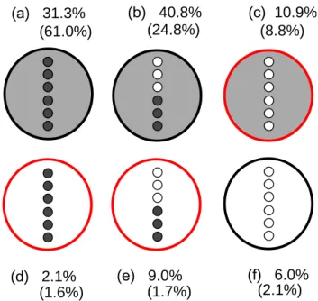
Fig. 3. Six general scenarios describe collocated AIRS and
Cloud-Sat/CALIPSO observations. Large gray (white) circles indicate cloudy (clear) AIRS FOVs. Small dark gray (white) circles indicate either cloudy (clear) CloudSat or CALIPSO profiles. The number and relative placement of small circles do not represent the actual number and locations of CloudSat and CALIPSO profiles within a given AIRS FOV, which vary substantially between FOVs. Cloud-Sat or CALIPSO profiles with rows of partly cloudy demonstrate heterogeneous cloud/clear scenes within an AIRS FOV. The rela-tive frequency of occurrence (in percent) for each scenario is shown separately for CloudSat and CALIPSO (in parentheses) for the five days listed in Table 1. The large red circles are candidates for “false” (Scenario C) or “failed” (Scenarios D and E) cloud detec-tions (AIRS relative to CloudSat or CALIPSO).
clouds when compared to the sensitivity from different spa-tial averaging approaches (Kahn et al., 2007a).
Clear sky and cloud frequency statistics for the three in-strument platforms are shown in Table 2. Most notable is the large difference in cloud frequency between CloudSat and CALIPSO. Although the CloudSat and CALIPSO data products have 1 and 5 km ground resolution, respectively, the majority of the difference is due to the relative sensitiv-ity of each instrument to hydrometeors that was discussed in Sect. 2. CloudSat reports the smallest frequency of clouds whereas AIRS demonstrates the greatest. That AIRS detects more clouds than CALIPSO is an indication of (1) some false cloud detections by AIRS, (2) missed clouds by CALIPSO, or (3) increases in FOV size lead to increases in perceived cloud frequency within some spatially heterogeneous cloud fields. Furthermore, a sensitivity of a few percent in AIRS frequency depends on the inclusion of the smallest values of
fA. CALIPSO cloud frequency statistics may depend on the
resolution of the feature mask (333 m, 1 km, and 5 km) but are not explored here.
0.15
0.10
0.05
0.00
AIRS Lower Layer Freq
(C) 20 15 10 5 0 Height (km) 0.15 0.10 0.05 0.00
AIRS Upper Layer Freq
(A) 20 15 10 5 0 Height (km) -60 -40 -20 0 20 40 60 Latitude (B) 0.12 0.10 0.08 0.06 0.04 0.02 0.00
AIRS Upper Layer f
A -60 -40 -20 0 20 40 60 Latitude 0.12 0.10 0.08 0.06 0.04 0.02 0.00
AIRS Lower Layer f
A
(D)
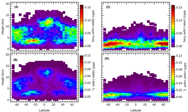
Fig. 4. Zonal average AIRS cloud frequency and fAfor the five days listed in Table 1. Latitude bins are 5◦in width and height bins are
0.5 km in depth. Cloud frequency PDFs are determined by counting the frequency of AIRS FOVs with fA≥0.005, whereas fAis the average
value (including clear sky) that is reported in the AIRS L2 Standard product. (a) AIRS upper layer frequency. (b) AIRS upper layer fA. (c)
and (d) as in (a) and (b) except for the AIRS lower layer.
To address the relative frequency of false and positive cloud detections, six general scenarios of coincidence are de-fined in Fig. 3. The frequency of occurrence for each sce-nario is shown, which account for heterogeneous and homo-geneous cloud fields within an AIRS FOV at any altitude in the vertical column. “False” (Scenario C) or “failed” (Sce-narios D and E) cloud detections occur approximately 22.0% (12.1%) of the time for CloudSat (CALIPSO) comparisons. Some cases are explained by the insensitivity of CloudSat to thin Ci (Scenario C) and the inability of AIRS to detect some low clouds such as Sc and Cu (Scenarios D and E), while others are explained by partial cloud adjacent to the Cloud-Sat/CALIPSO ground track within the AIRS FOV (Sce-nario C; e.g. Kahn et al., 2005), co-registration/collocation uncertainties (e.g. Kahn et al., 2007b), and other factors. For the five days in Table 1, averages of 19.3 and 10.6 Cloud-Sat profiles containing cloud (6.0 and 4.3 CALIPSO 5 km profiles) are located within a typical AIRS FOV for Scenar-ios (B) and (E), respectively. With regard to thin Ci, the CALIPSO comparison in Scenario C demonstrates a signifi-cant portion of either false AIRS detection (see Sect. 4.2) or clouds located outside of the CALIPSO ground track. In sce-narios D and E, many of these cases are thin Ci detected by CALIPSO that are below the detection limit of AIRS. Further analysis using (for instance) MODIS radiances is required to quantify the relative contributions to false and failed AIRS detection frequency.
Table 2. Percentage of clear and cloudy occurrences for
Cloud-Sat, CALIPSO, and AIRS. CloudSat cloud frequency is based on whether one or more range bins have a cloud confidence mask ≥20. AIRS cloud frequency is based on whether either the upper or lower
layer contains fA≥0.01 or fA≥0.0. CALIPSO cloud frequency is
based on the 5 km feature mask and whether at least one feature is detected in a given profile. These values do not represent the true global climatology because of the small sample (5 days), and the fact the days chosen are on the 16-day orbit repeat cycle, leading to potential spatial sampling biases.
Instrument % Clear % Cloudy
CloudSat 48.1 51.9 CALIPSO 22.7 77.3 (5 km) AIRS 19.6 80.4 (fA≥0.01) AIRS 17.1 82.9 (fA>0.0)
For Scenarios D and E (instances when the radar senses clouds and AIRS does not), the cloud types that dominate the missed cloud detections are assessed. For Scenario D (E), the percentage of missed St is 55% (70.1%) of all cloud types, respectively. This is not a surprise given that St dominates the overall frequency statistics (Wang and Sassen, 2007). Furthermore, the AIRS channel list was modified for V5 in
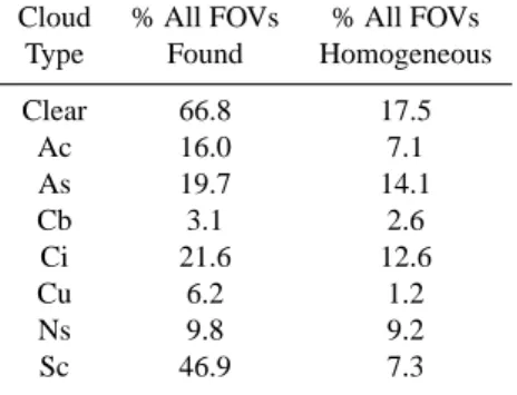
Table 3. Shown are the percentage of AIRS FOVs that contain at
least one CloudSat profile with these particular cloud types (mid-dle column), and the percentage of homogenous FOVs for the same cloud types (right column). A total of 52 320 AMSU FOVs and
2.37×10⁶CloudSat profiles (about 45 CloudSat profiles per AMSU
FOV) are used in this comparison for the 5-day period listed in Ta-ble 1.
Cloud % All FOVs % All FOVs
Type Found Homogeneous
Clear 66.8 17.5 Ac 16.0 7.1 As 19.7 14.1 Cb 3.1 2.6 Ci 21.6 12.6 Cu 6.2 1.2 Ns 9.8 9.2 Sc 46.9 7.3
such a way to be less sensitive to low clouds, hence increas-ing missed St detections over V4 that is to be discussed in Sect. 4.3. For Scenario D (E), As explains 23.7% (22.7%) missed cloud detections, while Ac composes 5.9% (3.6%) of all cases. Approximately 14.5% (1.6%) of Ns clouds ex-plain missed detections; the difference in percentages be-tween Scenarios D and E are largely explained by the fre-quency of homogeneous Ns clouds within the AIRS FOV (see Table 3). Missed detections of Ns are consistent with limitations of the AIRS algorithm in the presence of precip-itating clouds (Kahn et al., 2007a). All other cloud types explain about 1.5% or less of the missed cloud detections by AIRS. For instance, it is very rare that CloudSat detects Ci cloud when AIRS does not.
According to Scenarios B and E, the AIRS FOV is het-erogeneous 49.8% of the time using coincident radar-derived cloud profiles, but is reduced to 26.5% using lidar profiles. The higher sensitivity of lidar in detecting small hydrom-eteors suggests a lower frequency of clear sky/cloud het-erogeneity on the scale of the AIRS FOV than implied by the radar. Regardless of the instrument sensitivity, a sig-nificant percentage of AIRS observations contain heteroge-neous mixtures of clear and cloudy sky. The frequency of each cloud type detected within an AIRS FOV and the per-centage of homogeneous AIRS FOVs (where only one type occurs) are shown in Table 3. For AIRS FOVs that contain As, Cb, Ci and Ns a majority is homogeneous; in contrast Ac, Cu, and Sc are substantially more heterogeneous. Cloud profiles with vertically heterogeneous cloud types will be explored upon release of the combined CloudSat/CALIPSO cloud type mask and are not presented here.
3.2 A global five-day climatology
Figure 4 shows AIRS zonally averaged cloud frequency and
fA (defined in Sect. 2.1) from 70◦S–70◦N illustrating the
realism of AIRS cloud height (ZA), amount (fA), and
fre-quency. Cloud “frequency” is defined as the percentage of AIRS FOVs with non-zero fA. In the case of Fig. 4, cloud
frequency is partitioned into vertical bins, which sum to the values shown in Fig. 5. Although the biases of ZA
rela-tive to the radar are not appreciably different in the Polar latitudes, the rate of “false” or “failed” cloud detections is greatly increased (31%) compared to all latitudes (22%). The reasons for poorer cloud retrievals in high latitudes are be-ing explored and will be presented elsewhere. Figure 4a and b (4c and d) illustrates cloud frequency and fA for
the upper (lower) layer, respectively. Familiar global- and regional-scale cloud distributions are revealed. High cloudi-ness is most frequent in the tropical upper troposphere and mid-latitude storm tracks, whereas low cloud occurs within the subtropics extending to the high latitudes. Furthermore, minima in cloud frequency and amount are observed in the subtropical middle and upper troposphere. These patterns are qualitatively consistent with other climatologies (Rossow and Schiffer, 1999; Wylie et al., 1999; Thomas et al., 2004).
Zonally averaged cloud frequency and fA are shown in
Fig. 5a and b, respectively. Two minimum values of fA(0.0
and 0.01) used to define cloud in a frequency-based clima-tology (Fig. 4) illustrate the sensitivity to potentially spuri-ous cloud. Cloud frequency is 5–15% smaller (depending on latitude) using fAU<0.01 for the upper layer, however, the
corresponding change for fAL is only 1–2%. Zonally
aver-aged fA is lower with a global mean of ∼0.4 for the sum
of both layers, consistent with observations from the High Resolution Infrared Radiation Sounder (HIRS) (Wylie et al., 1999). We note that fractional global cloud cover is sub-stantially larger than 0.4, and fAincludes the effect of cloud
emissivity. Since many clouds do not radiate as black bodies, the average of fAis expected to be less than the true cloud
fraction (or frequency).
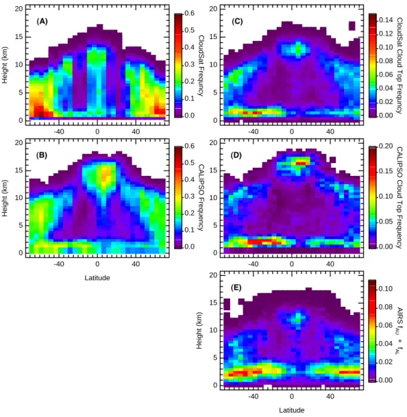
Zonally averaged cloud climatologies for collocated AIRS, CloudSat, and CALIPSO observations are illustrated in Fig. 6. The cloud distribution in Fig. 6 is not representative of any particular season or month (Table 1). CloudSat cloud frequency for mask values ≥40 is shown in Fig. 6a. The radar penetrates through nearly all clouds and high frequencies are present throughout the tropical column with the peak from 10–13 km. However, a climatology like that shown in Fig. 6a is not directly comparable to one derived from AIRS. A cli-matology of CloudSat-observed cloud tops using the high-est cloudy range bin within a given vertical profile is pre-sented in Fig. 6c. The cloud top climatology compares much more favorably with AIRS (Fig. 6e) as expected in terms of zonally-averaged spatial patterns and the magnitude of cloud frequency since AIRS does not sample the full vertical struc-ture of a given cloudy column. Likewise, CALIPSO cloud
frequency derived from the 5 km feature mask is shown in Fig. 6b, and the cloud top climatology is shown in Fig. 6d. As with CloudSat, the CALIPSO cloud top climatology qual-itatively agrees more favorably with AIRS, although height and sampling biases are apparent from inspection of the fre-quency patterns with respect to height and latitude, these will be explored in more detail in Sect. 4.
There are several additional notable features between AIRS and CloudSat/CALIPSO shown in Fig. 6. First, the peak frequency in the tropical upper troposphere is zonally offset between AIRS and CloudSat by ∼5◦. At least two explanations are possible: (1) the cloud types AIRS and the radar are most sensitive to are not uniformly distributed (i.e. Ci versus Cb) introducing a zonally-dependent sam-pling bias, and (2) precipitating clouds occasionally produce
ZA retrievals too low in the troposphere with erroneously
low values of fA (Kahn et al., 2007a). Second, AIRS
re-trieves tenuous clouds at higher altitudes than the radar in the subtropical latitudes, suggestive of either sensitivity to thin Ci with small ice particles and/or spurious AIRS re-trievals. Third, the radar observes high frequencies of low clouds 1–2 km in height in most latitude bands implying a positive height bias for low clouds sensed by AIRS. Fourth, a second layer within Ns from 2–3 km is frequently observed and is inconsistent with IR sensitivity, to be discussed further in Sect. 4.
Several of the radar-lidar differences that are pointed out in Fig. 2 are also observed in Fig. 6. Cloud tops in the upper troposphere observed by the lidar are higher than the radar by 1–4 km depending on the latitude, and are more verti-cally extensive than observed by AIRS and the radar. This feature is more expansive from 15 S–15 N, whereas the peak frequency is shifted 5 N (10 N) relative to AIRS in Fig. 6a– b. However, a more appropriate cloud top boundary-based cloud climatology in Fig. 6c–e shows that the tropical cloud features compare much better. The broader zonal extent in the lidar climatology is expected because of high sensitivity to thin Ci. The northward shift is consistent with vertically thick and tenuous Ci layers persisting along the edge of the ITCZ allowing the lidar to detect higher cloud frequencies at lower altitude bins. The lower frequency of lidar-detected clouds from 5◦S–5◦N is a result of sampling biases. At this latitude, clouds are more frequently opaque and precipitating and the lidar observations are restricted to a narrow vertical range resulting in fewer detected clouds. Furthermore, the li-dar and rali-dar (Fig. 6a and b) observe low clouds across most latitudes, however, the radar observes more in the ITCZ and less in the Northern Hemisphere (NH) subtropics than the lidar. The low cloud frequency differences are likely a re-sult from a combination of sampling biases (e.g. upper cloud layers obscuring the lidar’s view of low cloud, the insensitiv-ity of radar to smaller droplets, etc.), and CloudSat’s limita-tions in the lowest 1.0–1.25 km in R03. Lastly, the frequency minima within subtropical gyres in Fig. 6a extend more pole-ward into the midlatitudes in Fig. 6b, consistent with the high
1.0 0.8 0.6 0.4 0.2 0.0 fA -60 -40 -20 0 20 40 60 Latitude (B) fAU fAL fAU + fAL 1.0 0.8 0.6 0.4 0.2 0.0 Cloud Frequency
Upper Layer Freq (fAU > 0.0)
Upper Layer Freq (fAU 0.01)
Lower Layer Freq (fAL > 0.0)
Lower Layer Freq (fAL 0.01)
(A)
Fig. 5. (a) Zonal average cloud frequency for both AIRS cloud
lay-ers (the total of all vertical bins in Fig. 4a and d) for all clouds
(fA>0) and screened for clouds most likely to be unphysical
(fA≥0.01). See the text for discussion on unphysical cloud
re-trievals. (b) As in (a) except for the two layers of fA and their
sum. No screening of fAis shown in (b).
opacity of clouds in the storm tracks.
4 Height differences partitioned by cloud type
While AIRS estimates up to two cloud layers, the verti-cal structure cannot be profiled in the manner of a radar or lidar, making comparisons less straightforward than some other studies (Mace et al., 1998; Miller et al., 1999). In this section, coincident cloud top height observations be-tween AIRS, CloudSat, and CALIPSO are differenced to quantify the precision of ZA as a function of fA and cloud
type. The resolution of CloudSat and CALIPSO is not de-graded to AIRS, instead each CloudSat and CALIPSO pro-file is compared to the nearest AIRS retrieval. Random sam-pling of one CloudSat profile per AIRS FOV demonstrates that the bias and variability are within ±0.1–0.3 km for the approach taken in this section. Furthermore, we show that biases and variability in cloud top differences among dif-ferent cloud types are several factors larger than those in-troduced from choosing a particular averaging methodology (Kahn et al., 2007a). More importantly, we will show that the differences among the different cloud types are several factors larger than biases and variability introduced by the
20 15 10 5 0 Height (km) -40 0 40 0.6 0.5 0.4 0.3 0.2 0.1 0.0 CloudSat Frequncy (A) 20 15 10 5 0 Height (km) -40 0 40 Latitude 0.6 0.5 0.4 0.3 0.2 0.1 0.0 CALIPSO Frequency (B) 20 15 10 5 0 Height (km) -40 0 40 Latitude 0.10 0.08 0.06 0.04 0.02 0.00 AIRS f AU + f AL (E) 20 15 10 5 0 -40 0 40 0.14 0.12 0.10 0.08 0.06 0.04 0.02 0.00
CloudSat Cloud Top Frequncy
(C) 20 15 10 5 0 -40 0 40 0.20 0.15 0.10 0.05 0.00
CALIPSO Cloud Top Frequency
(D)
Fig. 6. Zonal-height cross-sectional averages of the 5 days listed in Table 1 for (a) CloudSat cloud frequency using cloud confidence mask
values ≥40, (b) CALIPSO cloud frequency using feature base and height values from the 5 km cloud feature mask, (c) as in (a) except for only the highest cloudy CloudSat range bin (cloud top), (d) as in (b) except for the highest detected cloud top sensed by CALIPSO (cloud
top), and (e) a combined AIRS upper and lower fA (sum of Fig. 4b and d). All latitude and height bins are in 5◦and 0.5 km increments,
respectively.
choice of sampling strategy. Approximately 45–50 CloudSat profiles (9–10 CALIPSO) coincide with the AIRS FOV. A “nearest neighbor” collocation approach is applied using lat-itude/longitude pairs. The gap between AIRS nadir view and CloudSat and CALIPSO depends on latitude. As a result, an AIRS FOV occasionally contains less than 45–50 CloudSat and 9–10 CALIPSO match-ups since the index of the col-located footprint is not constant with successive scan lines. Fields of fAare averaged to the resolution of ZA. Additional
challenges of collocating multiple satellite measurements are addressed further in Kahn et al. (2007b).
4.1 CloudSat–AIRS
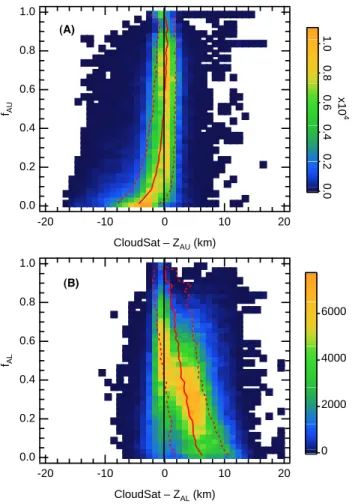
Globally averaged differences of AIRS upper (ZAU) and
lower (ZAL)cloud layers with radar-derived cloud top height
(ZCS)are shown in Fig. 7. About 72.1% of AIRS FOVs are
comparable to CloudSat, following Scenarios A and B pre-sented in Fig. 3; the remaining FOVs are clear or represent false or failed detections, which encompass several possibil-ities (see Sect. 3). The ZCS is the highest altitude range bin
with a confidence mask ≥20; no other cloud layer detected by the radar is used in the comparison, even in the presence of additional layers. The cloud type associated with the high-est range bin classifies the comparisons by cloud type. As
1.0 0.8 0.6 0.4 0.2 0.0 fAL -20 -10 0 10 20 CloudSat – ZAL (km) 6000 4000 2000 0 (B) 1.0 0.8 0.6 0.4 0.2 0.0 fAU -20 -10 0 10 20 CloudSat – ZAU (km) 1.0 0.8 0.6 0.4 0.2 0.0 x10 4 (A)
Fig. 7. Joint probability density functions of CloudSat-AIRS cloud
top height differences (for the days listed in Table 1) as a function
of fA. (a) CloudSat-AIRS height differences (1Z) using the AIRS
upper cloud layer (ZAU). (b) As in (a) except the AIRS lower cloud
layer (ZAL)is used. For a given vertical profile, the CloudSat cloud
top is defined as the highest altitude in which a cloud confidence
mask value ≥20 (both (a) and (b) use the same value). ZAU and
ZAL are calculated from the cloud top pressure and geopotential
height fields in the AIRS L2 Standard files. The solid red line is the
mean value of 1Z for each fAbin and the dashed red lines are the
±1 σ variability.
discussed in Sect. 3, a histogram approach like that taken by Kahn et al. (2007a) to account for multiple radar-derived cloud layers, changes the biases and variability by a smaller amount than those found between different cloud types.
Figure 7a and b shows differences of ZCS–ZAU≡1ZU
and ZCS–ZAL≡1ZL, respectively, as a function of fA
av-eraged over all cloud types. The variability is greater (espe-cially for 1ZU>0) if the confidence mask is relaxed to
val-ues less than 20 (not shown). Figure 7a shows that 1ZU
is a strong (weak) function of fAU<0.2 (fAU>0.2). The
mean bias (solid red line) is −1.0 to −4.0 km for fAU<0.2,
increasing to 0.5 km as fAU approaches 1.0. Likewise,
the variability (dashed red lines) ranges from ±3.5 km for
Table 4. Summary of CloudSat–AIRS cloud top differences shown
in Figs. 7–10. Bias and variability (±1 σ ) are in km. “AIRS Layer” indicates the layer that most accurately captures a particular cloud type.
Cloud AIRS Bias ±1 σ
Type Layer Variability
All Upper 4.0 to 0.2 1.2–3.6 All Lower 0.1 to 6.2 1.8–4.5 Ac Upper 4.0 to 0.2 0.7–3.0 As Upper 2.3 to 0.7 0.9–2.6 Cb Upper 1.4 to 1.6 0.9–4.0 Ci Upper 0.2 to 1.5 1.1–2.8 Cu Lower 0.3 to 1.5 0.3–2.2 Ns Upper 3.3 to 0.4 0.7–2.5 Sc Lower 1.3 to 0.3 0.4–1.7
fAU∼0.01 to ±1.25 km for fAU∼1.0. There are two
con-tributing factors to the negative bias for fA<0.2: (1) the
radar is insensitive to thin and tenuous Ci layers that AIRS detects above lower cloud layers that the radar detects, and (2) some of the small fAU retrievals are spurious. In Fig. 7b,
two broad clusters are suggested for 1ZL. As fALincreases,
1ZLdecreases for the cluster with smaller fALbecause the
lower layer becomes the dominant cloud layer. The clus-ter with higher fAL is centered near 1ZL∼0 km and is
in-dependent of fAL. This second cluster suggests that AIRS
retrieves a quantitatively meaningful lower cloud layer. We will show that the second cluster is associated with particular cloud types.
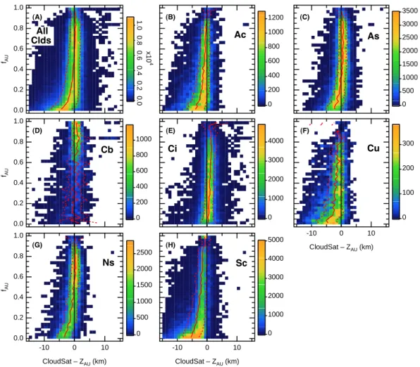
The results in Fig. 7a are partitioned into individual cloud types using the 2B-CLDCLASS product and are shown in Fig. 8. Several differences of 1ZU among the assorted cloud
types are observed. First, the negative bias for low fAU in
Fig. 7a is primarily due to Sc (the count in Fig. 8h exceeds Fig. 8b–g), with additional contributions from Ac, Cu, and Ns. For these cases the radar detects low or middle clouds while ZAU is located at a higher altitude. Some ZAU are
physically plausible (e.g. thin Ci residing over Sc or Cu in the subtropics or tropics) and some are spurious (to be discussed in Sect. 4.2). Second, the magnitude of fAU for individual
cloud types is qualitatively consistent with expectations. For instance, Cb is dominated by fAU>0.8 (low values occur for
partial coverage in the AIRS FOV), Ci is 0.05<fAU<0.4,
and Ns is in between Cb and Ci with 0.5<fAU<0.9. Few
cases of Ns with fAU>0.9 are observed because non-zero
fALseveral km below the Ns cloud top is frequently retrieved
(fAL+fAU typically sum to 1.0); a similar tendency is also
observed within some Cb as well (see Fig. 2). Ac has a lower range of fAU compared to As, consistent with the
classifica-tion used in Rossow and Schiffer (1999) and the increased heterogeneity of Ac (Table 3).
-10 0 10 CloudSat – ZAU (km) 5000 4000 3000 2000 1000 0 (H) Sc 1.0 0.8 0.6 0.4 0.2 0.0 fAU -10 0 10 CloudSat – ZAU (km) 2500 2000 1500 1000 500 0 (G) Ns -10 0 10 CloudSat – ZAU (km) 300 200 100 0 (F) Cu 4000 3000 2000 1000 0 (E) Ci 1.0 0.8 0.6 0.4 0.2 0.0 fAU 1000 800 600 400 200 0 (D) Cb 3500 3000 2500 2000 1500 1000 500 0 (C) As 1200 1000 800 600 400 200 0 (B) Ac 1.0 0.8 0.6 0.4 0.2 0.0 fAU 1.0 0.8 0.6 0.4 0.2 0.0 x10 4 (A) All Clds
Fig. 8. CloudSat-ZAU (for the days listed in Table 1) as a function of AIRS fAU. (a) Repeat of Fig. 7a. (b) Portion of PDF in (a) where the cloud classification indicates Altocumulus (Ac) clouds at the CloudSat cloud top (as defined in the caption of Fig. 7); there is no partitioning of CloudSat profiles that may contain one or more vertically-stacked cloud types. (c) Altostratus (As). (d) Cumulonimbus (Cb). (e) Cirrus (Ci). (f) Cumulus (Cu). (g) Nimbostratus (Ns). (h) Stratocumulus (Sc). The relative frequencies of each cloud type are given by the magnitudes of each PDF; further frequency statistics on cloud-type frequencies are given in Wang and Sassen (2007). The solid and dashed red lines are the mean and ±1 σ variability, respectively, as in Fig. 7.
Third, both bias and variability strongly depend on cloud type. Sc and Cu have negative 1ZU, consistent with the high
height biases shown for low clouds in Fig. 6. Cb and Ci (and As and Ns for higher values of fAU) have positive biases
of 1ZU. Holz et al. (2006) showed that Ci cloud top
re-trievals derived from IR measurements are frequently placed 1–2 km or more below the physical cloud top. Likewise, Sherwood et al. (2004) showed that height differences de-rived from geostationary imagery and coincident lidar are 1– 2 km even within highly opaque cloud tops. The variability in bias decreases as fAU increases for all cloud types except Ci,
which remains somewhat constant with fAU. The variability
is smallest for As, Ci, and Ns (for fAU>0.5) and largest for
Cb (fAU<0.6), Cu (fAU<0.4), and Sc (fAU<0.4).
Further-more, As shows less variability than Ac. Therefore, more heterogeneous clouds (see Table 3) tend to have larger vari-ability in 1ZU.
Figure 9 shows the results for 1ZL. The cluster at small
fALis dominated by As, Cb, Ci, and Ns. Whether ZALis a
physically reasonable second cloud layer, or a consequence of retrieval algorithm limitations, it is expected that vertical profiles of IWP derived from the radar will provide further insight on ZAL. In R03, CloudSat IWP retrievals in thick
and/or precipitating clouds are not reported which hinders the exploration of ZAL within Cb and Ns; however, an
im-proved retrieval is anticipated for the R04 release (2B-CWC-RO R03 data quality statement at http://www.cloudsat.cira. colostate.edu). Sc clouds dominate the cluster with high fAL
(see the high count in Fig. 9h) with contributions from Ac and Cu. ZALagrees best with the radar in low and middle
al-titude liquid water clouds. For Ns clouds, the bias in ZALis
lower as fALincreases, resulting in two cloud layers in close
vertical proximity when fALis large. Despite the complexity
1400 1200 1000 800 600 400 200 0 (B) Ac 2500 2000 1500 1000 500 0 (C) As 1.0 0.8 0.6 0.4 0.2 0.0 fAL 6000 4000 2000 0 (A) All Clds 1.0 0.8 0.6 0.4 0.2 0.0 fAL 600 500 400 300 200 100 0 (D) Cb 2000 1500 1000 500 0 (E) Ci -10 0 10 CloudSat – ZAL (km) 400 300 200 100 0 (F) Cu 1.0 0.8 0.6 0.4 0.2 0.0 fAL -10 0 10 CloudSat – ZAL (km) 2500 2000 1500 1000 500 0 (G) Ns -10 0 10 CloudSat – ZAL (km) 4000 3000 2000 1000 0 (H) Sc
Fig. 9. As in Fig. 8 except for ZAL. The CloudSat cloud top and cloud type are the same as shown in Fig. 8.
AIRS is shown to possess skill in detecting and assigning an altitude to low cloud layers.
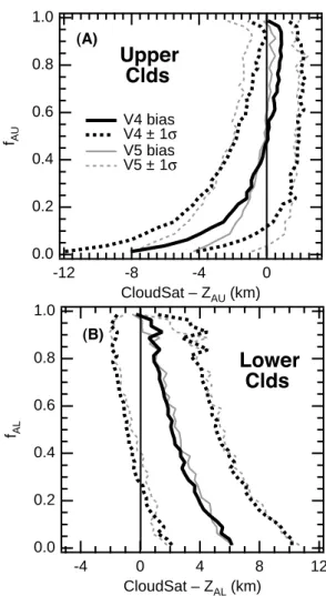
Figure 10 shows mean bias and variability statistics for V4 and V5 AIRS retrievals, and the results for V5 are summa-rized in Table 4. In Fig. 10a, the bias is substantially smaller for fAU<0.1 and fAU>0.6 in V5. This demonstrates that
improvements to cloud retrievals were made for V5. The larger negative bias for fAU<0.1 in V4 was primarily a
re-sult of poorer retrievals in Ac and Ci (not shown). The larger positive bias in V4 for fAU>0.6 was a result of poorer
re-trievals in As and Ns, and to a lesser extent, Ci and Cu (not shown). However, in the case of Sc, the V5 bias is larger by 0.25–0.5 km depending on the magnitude of fAU.
Dif-ferences in day-night and land-ocean biases and variability were explored. Between day and night, as well as between land and ocean, these differences are not qualitatively sig-nificant and are several factors smaller than the differences between V4 and V5 (not shown).
4.2 CALIPSO-AIRS
Given the known differences in lidar and radar sensitivity,
ZA and lidar-derived cloud top height (ZCAL) differences
(1ZCAL)have the potential to be significantly different than
demonstrated in Sect. 4.1 with the radar. However, Fig. 11 reveals qualitatively similar distributions compared to Fig. 7. The sum of Fig. 11a and b (11c and d) is analogous to Fig. 7a (7b). Clouds are partitioned into two categories with
ZCAL<7 km and ZCAL≥7 km. About 85.8% of AIRS FOVs
are comparable to CALIPSO, following Scenarios A and B presented in Fig. 3; as discussed in Sect. 3 the remaining FOVs are clear or represent false or failed detections. In Fig. 11a, the bias of 1ZCALis 1–3 km with high values for
small fAU. The variability is relatively large for small fAU
with most of the scatter skewed towards ZCAL>0. This
reaf-firms the sensitivity of lidar to tenuous clouds and the ten-dency for IR-derived cloud tops to be located within the mid-dle or lower portions of Ci layers (Holz et al., 2006).
Differences between Figs. 7a and 11 reveal the following about the lidar-AIRS comparisons in Fig. 11b: (1) the nega-tive bias for small fAU is greater by 2 km, (2) the variability
1.0 0.8 0.6 0.4 0.2 0.0 fAU -12 -8 -4 0 CloudSat – ZAU (km) (A)
Upper
Clds
V4 bias V4 ± 1σ V5 bias V5 ± 1σ 1.0 0.8 0.6 0.4 0.2 0.0 fAL 12 8 4 0 -4 CloudSat – ZAL (km) (B)Lower
Clds
Fig. 10. Bias (solid) and ±1 σ variability (dashed) of
CloudSat-AIRS ZAdifferences for V4 (black) and V5 (red).
is smaller by 0.5–1.0 km, and (3) the largest negative biases are limited to a smaller range of fAU. The radar’s
insensi-tivity to small hydrometeors is consistent with (3). Another implication of (3) is that ZAU is “reasonable” (although
bi-ased in altitude) for many tenuous Ci. This is also suggested by (2) since slightly lower variability is observed with the lidar comparisons, which are more accurate observations of “true” cloud top boundary than radar. Both (1) and (3) sug-gest many spurious cloud retrievals in the upper troposphere for fAU<0.02. However, the percentage of spurious
re-trievals is variable and generally decreases as fAU increases
and are not necessarily restricted to fA<0.02. The
likeli-hood is small that heterogeneous AIRS FOVs explain a sig-nificant portion of the large negative bias for fAL<0.02 since
sub-pixel heterogeneity tends to increase variability, not nec-essarily bias (Kahn et al., 2007b). In Fig. 11b, the bias in
1ZCALranges from −2 to −0.5 km as fAU increases from
0.2 to 1.0, whereas the variability is somewhat smaller than
1ZU in Fig. 7a. Overall, ZA shows positive height biases
for low clouds and negative height biases for high clouds
rel-Table 5. Summary of CALIPSO-AIRS cloud top differences shown
in Fig. 11. Bias and variability (±1 σ ) are in km.
CALIPSO AIRS Bias ±1 σ
ZCLD Layer Variability
>7 km Upper 0.6 to 3.0 1.2–3.6
>7 km Lower 6.5 to 10.8 1.2–4.0
≤7 km Upper −5.8 to −0.2 0.5–2.7
≤7 km Lower −0.7 to 1.0 0.5–2.8
ative to the radar and lidar (although the negative bias for high clouds is larger in the lidar comparisons and smaller for low clouds).
Figure 11c and d reveals a tendency for two height clusters as with Fig. 7b. In Fig. 11c (ZCAL≥7 km), ZAL is
consis-tently several km below cloud top, consistent within As, Cb, Ci, and Ns shown in Fig. 9. In Fig. 11d (ZCAL<7 km), ZALis
roughly equal to ZCALover the range of fAL, which
resem-bles the second cluster in Fig. 7b. Since cloud classification is not applied in the lidar comparisons, certain cloud types cannot be shown to explain particular height biases. How-ever, Fig. 11d is consistent with Cu and Sc shown in Fig. 9, which implies (like the radar) that ZALis skillful in
retriev-ing a lower layer. The ranges of bias and variability for V5 are summarized in Table 5. As with the CloudSat compar-isons, a reduction in negative bias is seen in V5 for tenuous clouds, and day/night and land/ocean differences in bias and variability are much smaller than V4 and V5 differences (not shown).
4.3 Changes in V5 AIRS retrievals and impacts on clouds Some of the algorithm changes to V5 have the potential to impact cloud retrievals, which include: limiting chan-nel selection for cloud clearing and cloud retrieval to 665– 811 cm−1, treating CO2as a global and time-dependent
con-stant, updating spectroscopic parameters like O3and HNO3
that affect transmittance in the cloud clearing channels, changing the approach to the downwelling IR radiance term, reducing the number of cloud height retrieval iterations dur-ing cloud cleardur-ing from 4 to 3, removdur-ing the ad hoc error term that impacts the damping parameters for cloud height retrievals (Susskind et al., 2003), and changing the basis of the empirical bias adjustment. The empirical bias correction in V4 used ECMWF analysis fields and in V5 the correction was derived from radiosondes launched during AIRS over-passes that coincided with intensive fields campaigns (Tobin et al., 2006).
The adjustments in the channel list were motivated in large part to eliminate window channels that have large contribu-tions of radiance from the surface. Retrieval yield and pre-cision over surfaces with large spectral emissivity features were improved, but the sensitivity to low clouds was reduced,
1.0 0.8 0.6 0.4 0.2 0.0 fAU -20 -10 0 10 20 CALIPSO – ZAU (km) 600 500 400 300 200 100 0 (A) CALIPSO 7 km -20 -10 0 10 20 CALIPSO – ZAL (km) 1000 800 600 400 200 0 (B) CALIPSO < 7 km -20 -10 0 10 20 CALIPSO – ZAL (km) 350 300 250 200 150 100 50 0 (D) CALIPSO < 7 km 1.0 0.8 0.6 0.4 0.2 0.0 fAL -20 -10 0 10 20 CALIPSO – ZAL (km) 350 300 250 200 150 100 50 0 (C) CALIPSO 7 km
Fig. 11. CALIPSO-AIRS 1Z. Cloud top height derived from CALIPSO is the highest cloud top found within the 5 km feature mask in a
given 5 km vertical profile.
including oceanic stratus. Thus, the sample size of AIRS and CloudSat comparisons for Sc clouds was smaller from V4 to V5. For instance, the frequency of occurrence of Sc within the dominant subtropical subsidence regions has decreased by as much as 10–20%. The comparisons presented here only consider cases when AIRS and CloudSat/CALIPSO si-multaneously observe cloud; it should be emphasized that the V4/V5 differences in Fig. 10 do not include observations when one of the instruments and/or data versions does not sense clouds.
CO2 was assumed to be globally constant at 370 ppm in
V4. However, in V5 the treatment of CO2 was changed to
a globally constant linear trend that increases as a function of time, but is without seasonal or latitudinal variation. In the case of high clouds, sensitivity tests have shown that thin cloud frequency is impacted for changes of 5–10 ppm, typ-ical for regional and seasonal variability, while very little change in fA is observed (consistent with a 5 ppm change
equivalent to 0.4 K in BT). The appearance (disappearance) of spurious (physically reasonable) Ci is observed when CO2
levels are assumed to be too low (high) in the forward model (Hearty et al., 2006). In practice, many thin Ci are placed
near the tropopause in otherwise clear sky in retrieved cloud fields. Erroneous values of CO2are likely to have some
im-pact on the misplaced cloud height for very low values of fA
seen in Fig. 11. Regarding middle and low clouds, signifi-cant changes are observed in fA, not only the frequency, in
the CO2sensitivity tests (Hearty et al., 2006). This
demon-strates the need for a more realistic estimate of CO2in the
forward model and suggests the potential utility of a simulta-neous CO2retrieval (Chahine et al., 2006) to more accurately
retrieve cloud amount and height.
Since the AIRS cloud retrieval steps are initialized with two cloud layers (350 and 850 hPa with fA of 0.167 and
0.333, respectively), the cloud-clearing algorithm must itera-tively “remove” cloud to produce cloud-cleared radiances for downstream retrievals of atmospheric and surface quantities. In a regularized algorithm like that discussed in Susskind et al. (2003), residual fA may be present in clear scenes
because the effectiveness of cloud clearing is limited (in part) by the magnitude of noise in the observed radiances. Thus, small amounts of residual cloud may remain for some clear FOVs. Lastly, global-scale trends of cloud frequency in V5 are greatly reduced over V4 (T. Hearty, personal
communication), although the lack of seasonal and latitu-dinal variability in CO2likely creates regionally dependent
biases in cloud frequency since cloud type and frequency are not distributed uniformly around the globe (e.g. Rossow and Schiffer, 1999; Wylie et al., 1999). Both CALIPSO and CloudSat will continue to play important roles in ongoing assessments of AIRS reprocessing efforts.
5 Conclusions
The precision of cloud height derived from the Atmospheric Infrared Sounder (AIRS), located on EOS Aqua, is explored and quantified for a five-day set of observations. Coincident profiles of vertical cloud structure by CloudSat, a 94 GHz profiling radar, and the Cloud-Aerosol Lidar and Infrared Pathfinder Satellite Observation (CALIPSO) determine the precision of AIRS-derived clouds in a wide variety of geo-physical conditions. By fitting simulated and observed spec-tral radiances, the AIRS retrieval algorithm derives up to two layers of cloud height (ZA)and effective cloud fraction (fA).
Comparisons are shown for both cloud layers and the entire range of fA. The cloud confidence and classification masks
reported by CloudSat determine cloud occurrence and height and allow the comparisons to be partitioned by cloud type. The 5 km cloud feature mask from CALIPSO is used for the same five-day set of collocated observations.
The CloudSat-AIRS biases and variability strongly depend on cloud type, ZA and fA. Using Version 5 (V5) AIRS
re-trievals, the cloud top biases range from −4.3 to 0.5 km ±1.2 to 3.6 km, depending on fAand cloud type. Large negative
biases occur for the smallest values of fAand small positive
biases for large fA. Likewise, the largest variability occurs
for the smallest fAand the smallest variability occurs for the
largest values of fA. Therefore, AIRS cloud top height is
shown to excel for most cloud types with relatively high val-ues of fA. Given that the cloud classification scheme used
in this work is developed from radar observations, the sensi-tivity of AIRS to particular cloud types is based strictly on clouds observed by CloudSat. The upper cloud layer has the highest sensitivity to Altocumulus, Altostratus, Cirrus, Cumulonimbus, and Nimbostratus cloud types and the lower layer to Cumulus and Stratocumulus. The bias and variability for individual cloud types vary widely, but almost all cloud types show reductions in biases and variability with increas-ing fA. Furthermore, a tendency for high (low) clouds to be
biased low (high) in height is shown. Frequently, two layers of ZAare retrieved within Nimbostratus, and to a lesser
de-gree, Cumulonimbus. The lower layer is not necessarily con-sistent with a physically plausible lower cloud layer. Some cloud types like thin Cirrus, Cumulus, and Stratocumulus are very challenging to characterize with IR measurements. The results presented herein suggest that AIRS has skill in detect-ing and assigndetect-ing cloud top heights to these difficult cloud types. For instance, the bias and variability of Cirrus,
Cu-mulus, and Stratocumulus are 0.2 to 1.5±1.1–2.8 km, −0.3 to 1.5±0.3–2.2 km, and −1.3 to −0.3±0.4–1.7 km, respec-tively. However, AIRS V5 detects a smaller percentage of Sc fields in and around the major oceanic Stratus regions in the subtropics compared to V4.
CALIPSO-AIRS differences qualitatively agree with those from the CloudSat-AIRS comparisons. For CALIPSO cloud tops ≥7 km and <7 km, the biases and variability are 0.6– 3.0±1.2–3.6 km, and −5.8 to −0.2±0.5–2.7 km, respec-tively, with the largest biases and variability for the smallest values of fA. The tendency for high clouds to have low ZA
biases is increased using CALIPSO (rather than CloudSat), consistent with the lidar’s increased sensitivity over the radar to small particles in tenuous cloud top boundaries. Likewise, the high ZA biases for low clouds are reduced in
magni-tude. This demonstrates that both CloudSat and AIRS are not as sensitive to thin Ci and boundary layer clouds compared to CALIPSO. The large negative ZAbiases in the CloudSat
comparisons for low values of fA are increased (decreased)
in the CALIPSO comparisons for clouds <7 km (>7 km) in height. This demonstrates that ZA is more precise for
thin Cirrus than implied by the CloudSat comparisons alone. However, there are instances when CALIPSO does not agree with AIRS thin Ci retrievals, demonstrating the existence of spurious ZA in the upper troposphere. Significant
improve-ments in the AIRS V5 operational retrieval algorithm are demonstrated. Some of the algorithm changes made to V5 are highlighted, and those that could have impacted cloud retrievals are discussed.
In summary, we have demonstrated the utility of Cloud-Sat and CALIPSO to evaluate the precision of AIRS cloud retrievals and identified particular cloud types for improve-ment. Given the relatively favourable agreement between the active- and passive-derived cloud heights, the AIRS swath will be useful to supplement the near-nadir cloud climatol-ogy from CloudSat and CALIPSO. Furthermore, since the biases and variability of AIRS cloud height have been quan-tified as a function of cloud type, they will help to determine biases in cloud type-dependent microphysical and optical re-trievals derived from AIRS radiances and similar IR imagers and sounders because cloud vertical structure is required for these retrievals. The inter-comparison of these (and other) data sets is a necessary step towards a unified and global view of cloud properties and their validated error estimates. Acknowledgements. B. H. Kahn was funded by the NASA Post-doctoral Program during this study and acknowledges the support of the NASA Radiation Sciences Program directed by H. Maring. The authors thank the AIRS, CloudSat, and CALIPSO team members for assistance and public release of data products, two anonymous reviewers for helpful comments and suggestions, and in particular to P. Partain and S. Tanelli for useful discussions on CloudSat data products and interpretations. AIRS data were obtained through the Goddard Earth Sciences Data and
Infor-mation Services Center (http://daac.gsfc.nasa.gov/). CloudSat