HAL Id: hal-02298396
https://hal.archives-ouvertes.fr/hal-02298396
Submitted on 15 Jan 2021
HAL is a multi-disciplinary open access
archive for the deposit and dissemination of
sci-entific research documents, whether they are
pub-lished or not. The documents may come from
teaching and research institutions in France or
abroad, or from public or private research centers.
L’archive ouverte pluridisciplinaire HAL, est
destinée au dépôt et à la diffusion de documents
scientifiques de niveau recherche, publiés ou non,
émanant des établissements d’enseignement et de
recherche français ou étrangers, des laboratoires
publics ou privés.
February 2014 geomagnetic storm over north Africa
Khalifa Malki, Aziza Bounhir, Zouhair Benkhaldoun, Jonathan Makela,
Nicole Vilmer, Daniel Fisher, Mohamed Kaab, Khaoula Elbouyahyaoui, Brian
Harding, Amine Laghriyeb, et al.
To cite this version:
Khalifa Malki, Aziza Bounhir, Zouhair Benkhaldoun, Jonathan Makela, Nicole Vilmer, et al..
Iono-spheric and thermoIono-spheric response to the 27–28 February 2014 geomagnetic storm over north Africa.
Annales Geophysicae, European Geosciences Union, 2018, 36 (4), pp.987-998.
�10.5194/angeo-36-987-2018�. �hal-02298396�
Ann. Geophys., 36, 987–998, 2018 https://doi.org/10.5194/angeo-36-987-2018 © Author(s) 2018. This work is distributed under the Creative Commons Attribution 4.0 License.
Ionospheric and thermospheric response to the 27–28 February
2014 geomagnetic storm over north Africa
Khalifa Malki1, Aziza Bounhir1, Zouhair Benkhaldoun1, Jonathan J. Makela2, Nicole Vilmer3, Daniel J. Fisher2, Mohamed Kaab1, Khaoula Elbouyahyaoui1, Brian J. Harding2, Amine Laghriyeb1, Ahmed Daassou1, and Mohamed Lazrek1
1Oukaïmeden Observatory, High Energy Physics and Astrophysics Laboratory, FSSM, Cadi Ayyad University,
Marrakesh, BP 2390, Morocco
2Department of Electrical and Computer Engineering, University of Illinois at Urbana-Champaign, Urbana, Illinois, USA 3LESIA, Observatoire de Paris, PSL Research University, CNRS, Sorbonne Universités, UPMC Univ. Paris 06, Univ. Paris
Diderot, 5 place Jules Janssen, 92195 Meudon, France Correspondence: Khalifa Malki (malki.khalifa@gmail.com) Received: 13 March 2018 – Discussion started: 28 March 2018
Revised: 13 June 2018 – Accepted: 18 June 2018 – Published: 12 July 2018
Abstract. The present work explores the ionospheric and thermospheric responses to the 27–28 February 2014 geo-magnetic storm. For the first time, a geogeo-magnetic storm is explored in north Africa using interferometer, all-sky im-ager and GPS data. This storm was due to the arrival at the Earth of the shock of a coronal mass ejection (CME) as-sociated with the solar flare event on 25 February 2014. A Fabry–Perot interferometer located at the Oukaïmeden Ob-servatory (31.206◦N, 7.866◦W; 22.84◦N magnetic) in
Mo-rocco provides measurements of the thermospheric neutral winds based on observations of the 630 nm red line emission. A wide-angle imaging system records images of the 630 nm emission. The effects of this geomagnetic storm on the ther-mosphere are evident from the clear departure of the neu-tral winds from their seasonal behavior. During the storm, the winds experience an intense and steep equatorward flow from 21:00 to 01:00 LT and a westward flow from 22:00 to 03:00 LT. The equatorial wind speed reaches a maximum of 120 m s−1 for the meridional component at 22:00 LT, after the zonal wind reverses to the westward direction. Shortly after 00:00 LT a maximum westward speed of 80 m s−1was achieved for the zonal component of the wind. The features of the winds are typical of traveling atmospheric disturbance (TAD)-induced circulation; the first TAD coming from the Northern Hemisphere reaches the site at 21:00 LT and a sec-ond one coming from the Southern Hemisphere reaches the site at about 00:00 LT. We estimate the propagation speed
of the northern TAD to be 550 m s−1. We compared the winds to the DWM07 (Disturbance Wind Model) prediction model and find that this model gives a good indication of the new circulation pattern caused by storm activity, but devi-ates largely inside the TADs. The effects on the ionosphere were also evident through the change observed in the back-ground electrodynamics from the reversal in the drift direc-tion in an observed equatorial plasma bubble (EPB). Total electron content (TEC) measurements of a GPS station in-stalled in Morocco, at Rabat (33.998◦N, 6.853◦W), revealed
a positive storm.
1 Introduction
The Sun is the energy provider of our planet through electro-magnetic radiation, solar wind and the interplanetary mag-netic field (IMF). It is a highly variable star with sporadic events consisting of outbursts of huge amounts of energy. Large solar flares are associated with an impulsive release of a large amount of ionizing emissions (UV, EUV, X-rays) that change the physical properties of the ionosphere, which may have a big impact on telecommunication and navigation, on a very small timescale. Coronal mass ejections (CMEs) are explosive outbursts of billions of tons of plasma originat-ing from the corona. CMEs carry powerful magnetic fields and coronal plasma and are associated with shock waves.
CMEs take from 1 to 4 days to travel to Earth, and inter-act with the solar wind and the IMF during their propaga-tion. They can trigger geomagnetic storms when they inter-act with the Earth’s magnetic field. Solar particle events are a release of relativistic charged particles – mainly protons and electrons produced in association with the flare or by the CME-associated shock. A large coronal hole facing the earth can also cause a geomagnetic storm. Many changes occur in the magnetosphere when an intense surge of solar wind or a coronal mass ejection reaches the Earth. The geomagnetic field can become highly variable, and all the currents flow-ing through the magnetosphere and the ionosphere change rapidly. In response, the composition and dynamics of the ionosphere and the thermosphere are highly affected.
According to the World Meteorological Organization, “space weather” designates the physical and phenomenolog-ical state of the natural space environment, including the Sun and the interplanetary and planetary environments. The asso-ciated discipline aims at observing, understanding and pre-dicting the state of the Sun and of the planetary and inter-planetary environments and their disturbances, with partic-ular attention to the potential impacts of these disturbances on biological and technological systems. Our modern society depends on technological tools for telecommunication, nav-igation, positioning, space exploration and energy provision. The effects of space weather can cause satellite damage, radi-ation hazards to astronauts and airline passengers, telecom-munication problems, outages of power and electronic sys-tems and the endangerment of human life in our technical societies. As the importance of technology will inevitably in-crease in our daily lives there is a need to thoroughly under-stand the Sun/Earth system and space weather. The Interna-tional Space Weather Initiative (ISWI), a program of inter-national cooperation, was created to advance space weather science by a combination of instrument deployment, analysis and interpretation of space weather data.
It is within the framework of the ISWI program that the RENOIR (Remote Equatorial Nighttime Observatory of Ionospheric Region) experiment was deployed in Morocco on November 2013 at the Oukaïmeden Astronomical Ob-servatory of Cady Ayyad University (31.206◦N, 7.866◦W; 22.84◦N magnetic). The RENOIR experiment consists of a Fabry–Perot (FPI) interferometer and a wide-angle viewing camera. The FPI makes measurements of the thermospheric neutral wind velocities and neutral temperatures using ob-servations of the 630.0 nm emission caused by the dissocia-tive recombination of O+2. The wide-angle imaging system uses the same airglow emissions to provide measurements of ionospheric structures and irregularities. The main goal of this experiment is to characterize the midlatitude ionosphere and thermosphere by establishing the climatology of both the neutral winds and the instabilities taking place in the iono-sphere as well as the coupling between the ionoiono-sphere and thermosphere during quiet-time conditions and during geo-magnetic storms.
Thermospheric winds are driven primarily by pressure gra-dients due to the absorption of solar radiation and collisions between atmospheric constituents and precipitating auroral particles. During a geomagnetic storm, the energy input mod-ifies the global circulation of the thermosphere, which pro-foundly influences the structure and composition of the iono-sphere. Understanding the thermosphere–ionosphere cou-pling is the most challenging problem in space weather. It is within this context that we conduct thermospheric and ionospheric measurements over a midlatitude site in north Africa by using data from an interferometer, a GPS station and an all-sky imager. In the present paper, we analyze the ionospheric and thermospheric response to the 27–28 Febru-ary 2014 geomagnetic storm. We illustrate the evident de-parture of the neutral winds from their normal behavior. A reversal in the background ionospheric electric field was ev-ident through the dynamics of the plasma bubbles that oc-curred that night (Blanc and Richmond, 1980; Fejer et al., 2017). The drift velocity of the EPB (equatorial plasma bub-ble) is compared to the zonal neutral winds in order to in-vestigate the dynamo. Total electron content (TEC) measure-ments demonstrate the nature of the ionospheric storm pre-cisely. We have also conducted a comparison of the neutral winds with the DWM07 (Disturbance Wind Model) predic-tions. This is the first time that a case study of a geomagnetic storm has been achieved in north Africa by using Fabry– Perot interferometer data of the thermosphere. Additionally, this is the first coincident study of a storm using a ground-based FPI and an all-sky imager in this sector.
2 Source of the geomagnetic storm
On 25 February 2014 at 00:49 UT, an X4.9-class flare was produced in NOAA active region (AR) 1990 close to the east limb. It was associated with a halo CME, with a speed of more than 2000 km s−1 (see CDAW CME catalog, Yashiro et al., 2004). The flare–CME event produced a solar en-ergetic particle event observed by many spacecrafts (Lario et al., 2016). The CME-associated shock reached the Ad-vanced Composition Explorer (ACE) satellite on 27 Febru-ary 2014 at ∼ 16:00 UT (see e.g., Lario et al., 2016) with an increase in the density, temperature, velocity of the solar wind and the amplitude of the interplanetary magnetic field and an inversion of the Bz magnetic field component. The resultant geomagnetic storm was characterized by the vari-ations of the Kp, Dst (disturbance storm time) and auroral electrojet (AE) geomagnetic indices shown in Fig. 1. The Dst index is indicative of the total energy content of the particles responsible for the ring current. Geomagnetic storms with |Dst|max between 100 and 200 nT are classified as intense,
with |Dst|max>200 nT as super-intense and other events
with |Dst|max between 50 and 100 nT classified as
moder-ate (Singh et al., 2017). According to this classification, a moderate storm took place as observed during 27
Febru-K. Malki et al.: The 27–28 February 2014 geomagnetic storm over north Africa 989
Figure 1. Time variations of the Kp, Dst and AE geomagnetic indices for the period 25–28 February 2014.
ary 2014 at ∼ 16:30 UT with |Dst|max'90 nT associated
with the CME shock arrival. The AE index variations, based on high-latitude magnetograms (AE ∼ 400–500 nT weak ge-omagnetic activity and AE ∼ 1000 nT intense gege-omagnetic activity), also show moderate storm activity on 27 Febru-ary 2014 at 16:30 UT, with the AE index attaining values greater than 800 nT. The NOAA real-time observed Kp in-dex reached 5 during the synoptic period 16:00–18:00 UT on 27 February following the CME shock arrival. These intense variations in all geomagnetic indices are due to the arrival and interaction with Earth’s magnetosphere of the CME from NOAA AR 11990. As the energy is deposited into the Earth’s geospace system, effects are expected to propagate from high to low latitudes, modifying the Earth’s thermosphere– ionosphere system. Below, we use measurements obtained from an observatory in Morocco to study these changes at midlatitudes.
3 Data and instrumentation
Figure 2 shows the locations of the instruments used to col-lect data from the ionosphere and thermosphere. These in-struments consist of an FPI and a wide-angle camera (Makela et al., 2011) located at the Oukaïmeden Observatory in Mo-rocco (31.206◦N, 7.866◦W; 22.84◦N magnetic; 2700 m of altitude). The FPI alternates between observations of the
Figure 2. Viewing geometry (yellow circle) of the RENOIR exper-iment centered at Oukaïmeden Observatory (31.206◦N, 7.866◦W; 22.84◦N magnetic). The city of Rabat (33.998◦N, 353.1457◦E) locating a GPS system is included in the viewing area. The yellow triangles indicate the viewing directions of the Fabry–Perot inter-ferometer.
thermosphere at locations 250 km to the east, west, north and south of the observatory, and the viewing area of the cam-era covers a circle with ∼ 500 km radius. The city of Rabat
(33.998◦N, 6.854◦W) where the GPS is located is included in that viewing area.
The FPI measures the Doppler shifts and Doppler broaden-ings of the 630.0 nm spectral emission and infers the thermo-spheric wind and temperatures for an altitude around 250 km. To be able to collect incident light from any direction, a sys-tem of two parallel mirrors called a sky scanner is used which points in six directions during each cycle (laser, zenith, north, east, south and west). The incident light passes through a nar-rowband interference filter (630.0 nm) and an etalon before being focused onto the CCD (charge-coupled device) plane by a lens. An interference pattern is captured by the CCD and processed to produce estimates of the neutral wind ve-locity and temperature (Harding et al., 2014). A frequency-stabilized HeNe laser is used to provide an estimate of the instrument’s optical transfer function and to characterize the instrument’s drift over the night.
The all-sky imaging system consists of a lens system, a five position filter wheel and a CCD device. One filter is used to isolate the 630 nm emission, allowing plasma bub-bles, medium-scale traveling ionospheric disturbances, grav-ity waves and ionospheric irregularities in general to be visu-alized (Makela and Miller, 2008; Duly et al., 2013).
Numerous studies have shown that the GPS is an effec-tive tool for characterizing the ionosphere through measur-ing the TEC, which represents the total number of electrons integrated along the path from the receiver to each GPS satellite (Sethi et al., 2001; Boutiouta and Belbachir, 2006; Chauhan and Singh, 2010; Ouattara et al., 2011). Here, we present the vertical total electron content (VTEC) over Ra-bat (33.998◦N, 6.853◦W) obtained from the International GPS Geodynamics Service (IGS) network. The GPS data needed to determine the TEC are (1) data extracted from files stored in RINEX (Receiver INdependent EXchange) format, (2) data in IONEX format (IONosphere EXchange Format), (3) almanacs of the GPS satellite position and (4) the satel-lite clock biases. The procedure for extracting the TEC from GPS data is well documented in the literature (Sardon et al., 1994; Klobuchar, 1996; Schaer, 1999; Zoundi et al., 2012; Christian et al., 2013).
4 Thermospheric and ionospheric response 4.1 Thermospheric wind response
The day–night difference in the solar heating is the pri-mary source that controls the thermospheric wind circulation during quiet-time conditions. Another important secondary source is upward propagating tides. During geomagnetic storms, joule heating is enhanced by strong high-latitude electric currents and by collisions of neutrals with convect-ing ions. These highly variable sources cause disturbances to thermospheric winds which will further affect the global ionospheric dynamo (Blanc and Richmond, 1980). In dis-turbed geomagnetic conditions, thermospheric neutral winds
exhibit large deviations from their quiet-time climatologi-cal behavior and can drive large changes in the ionospheric plasma density, composition, temperature and electrodynam-ics (Richmond and Matsushita, 1975; Rishbeth and Edwards, 1989; Fuller-Rowell et al., 1994; Buonsanto, 1999; Emmert et al., 2004; Mendillo, 2006; Meriwether, 2008).
Before commenting on the behavior of thermospheric winds over Oukaïmeden Observatory during the study pe-riod (25 to 28 February 2014), we first begin by summarizing their basic climatology (Kaab et al., 2017). In summertime, the meridional winds are equatorward for the entire night, reaching a maximum speed of 75 m s−1. A poleward com-ponent is present in winter, in the early evening hours un-til 21:00 UT. The peak in equatorward flow shifts through-out the year from 23:00 UT during the spring equinox to 02:00 UT during the autumn equinox. The zonal winds are eastward during the entire night, with typical speeds around 50 m s−1 during the early evening hours, 75 to 100 m s−1 around 21:00 UT and almost zero before dawn in wintertime. A westward reversal is present shortly before dawn in local summer.
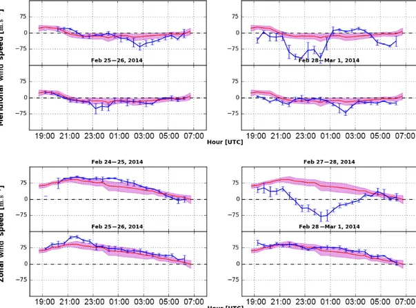
Figure 3 shows the geographic meridional and zonal winds measured with the FPI during 24, 25, 27 and 28 February 2014. The 26 February measurements are missing due to a power outage. The FPI measures line of sight (LOS) winds in four cardinal directions – east, west, north and south. The east and west LOS winds are zonal winds and the north and south LOS winds are meridional winds. The FPI data have been binned into half-hour bins. The error bars rep-resent variability (mean ± σ ) within each 30 min time bin. The quiet time refers to data with 3 h Kp < 4. The aver-age quiet-time wind components derived from measurements are in red, and the quiet-time daily variability is illustrated by the shaded purple area. Positive wind values are north-ward for the meridional winds and eastnorth-ward for the zonal ones, respectively. We can clearly notice that the effect of the storm on 27 February 2014 is very noticeable on both the meridional and zonal winds that have largely departed from their quiet-time climatology. Figure 1 indicates that Kp is low until ∼ 17:00 UT on 27 February, when Kp grows to 4 and eventually reaches 5. The meridional wind was equa-torward and increased sharply after 21:00 UT to a speed of about 140 m s−1and reversed sharply to a poleward direction around 01:00 UT. They remain poleward with a low speed until 04:00 UT, when they reverse again to an equatorward direction. Instead of being eastward during the entire night, the zonal wind (on 27 February) starts eastward in the early evening, with lower speeds than the quiet-time climatology, reverses westward at 22:00 UT, achieving a maximum speed of 100 m s−1around 00:00 UT, and reverses back to an east-ward direction around 03:00 UT.
The steep and abrupt changes in the meridional winds are the signature of thermospheric traveling atmospheric disturbances (TADs) flowing over the area covered by the Oukaïmeden FPI measurements. The first TAD coming from
K. Malki et al.: The 27–28 February 2014 geomagnetic storm over north Africa 991
Figure 3. Thermospheric geographic meridional and zonal winds measured by the Fabry–Perot interferometer (FPI) over Oukaïmeden Ob-servatory (31.206◦N, 7.866◦W; 22.84◦N magnetic). The FPI winds are estimated from the 630 nm airglow emission caused by dissociative recombination of O+2. The dates of measurements are the 24, 25, 27 and 28 February 2014. The red line refers to the monthly average of the nights with Kp strictly less than 4. The blue line shows the meridional (zonal) measurements during the night and the magenta area denotes the daily variability during February 2014.
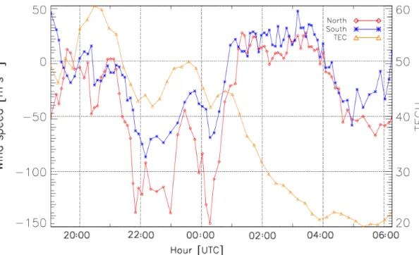
the Northern Hemisphere was captured around 21:00 UT, and the second TAD coming from the Southern Hemisphere was captured around 00:00 UT. At this point we find it inter-esting to represent the separate components of the merid-ional wind. Figure 4 shows the meridmerid-ional wind estimates made facing the north and south at an elevation angle of 45◦. These measurements are separated from one another by 500 km. In less than an hour the northern component of the wind gained a speed of almost 150 m s−1towards the equa-tor. The effect of the TAD coming from the North Pole lasted for about 4 h, during which the northern component had a higher speed than the southern one. The southern compo-nent reacted to the TAD with a delay of approximately 15 min. Our estimation then of the speed of the TAD over the studied area is about 550 m s−1. Xiong et al. (2015) used the superposed epoch analysis of CHAMP zonal wind observa-tions from 2001 to 2005 and estimated the typical propaga-tion speed of TADs to be 610 m s−1. From Fig. 4, the merid-ional winds reacted to the transequatorial southern TAD at 00:20. Its effect lasted for 3.5 h during which the southern lo-cation had a larger speed than the northern one. From 22:00 to 00:00 UT, the equatorward wind encountered some steep
reactive effects, especially from 23:00 to 00:00 LT, when the speed of the northern meridional wind lost about 100 m s−1 in 20 min. Usually the quiet-time northward surge of the wind related to the MTM (midnight temperature maximum) phenomenon occurred during that month (February 2014) on average between 22:30 and 00:30 UT with an average ampli-tude of 20 m s−1. The northward surge that occurred between 23:00 and 00:00 UT on 27 February 2014 might be due to the enhancement of the MTM phenomenon by the storm circu-lation.
The thermospheric response, induced by high-latitude heat input drives a global circulation of winds flowing from high to low latitudes (Buonsanto, 1989, 1990), creating large-scale atmospheric waves (Richmond, 1979) that propagate on a global scale. Due to Coriolis forces, a subsequent change in the zonal circulation flowing westward takes place. The storm-induced atmospheric waves propagates to low lati-tudes and into the opposite hemisphere. The local impression of this global picture of the storm was captured during the 27 February event (see Fig. 3). Indeed, the poleward surge oc-curred at 21:00 UT and drove the zonal wind to flow to the west at 22:00 UT. This result of westward and equatorward
Figure 4. Thermospheric north- and south-facing components of the meridional wind measured by the Fabry–Perot interferometer (FPI) over Oukaïmeden Observatory (31.206◦N, 7.866◦W; 22.84◦N magnetic).
winds during the magnetic storm is consistent with previ-ous results obtained using ground-based Fabry–Perot inter-ferometers (Makela et al., 2014; Zhang et al., 2015). Xiong et al. (2015) use the CHAMP zonal wind observations from 2001 to 2005 to investigate the global features of the distur-bance winds during magnetically disturbed periods. They re-port that the disturbance zonal wind is mainly westward and increases with magnetic activity and latitude. Emmert et al. (2004) report westward and equatorward nighttime disturbed winds at midlatitudes.
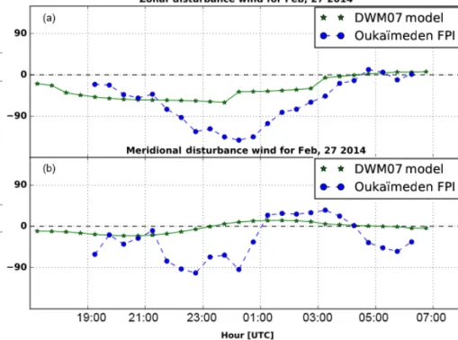
Emmert et al. (2008) present an empirical wind model (DWM07) representing average geospace-storm-induced perturbations of upper thermospheric neutral winds. In constructing their model, they used data from the Wind Imaging Interferometer on board the Upper Atmosphere Re-search Satellite, the Wind and Temperature Spectrometer on board Dynamics Explorer 2, and seven ground-based FPIs. The wind derived from their empirical model is dependent on three parameters: magnetic latitude, magnetic local time and the 3 h Kp geomagnetic activity index. To quantify the geomagnetically disturbed thermosphere, they established a quiet-time reference that they subtracted from each mea-surement (Emmert et al., 2008). We removed the average quiet-time wind from the wind measured on 27 February and compared this with the model prediction by DWM07 for this storm. Results are shown in Fig. 5. The model predicts westward disturbed zonal winds with a maximum speed of 60 m s−1from 19:00 UT until 03:00 UT. The measured dis-turbance wind is westward during the whole night but with a maximum speed of 140 m s−1around 00:00 UT. The speed
is then much higher than expected by the DWM07 empir-ical model. The meridional disturbed wind is clearly equa-torward (Fig. 5) until 00:00 UT, with a particularly steep increase starting at 21:00 UT, reaching a maximum speed of 90 m s−1 at 22:30 UT. An abrupt decreasing meridional speed occurs shortly after 00:00 UT, reversing the disturbed winds to a northward direction at 01:00 UT. However, the predicted meridional winds are extremely low, with a reversal time of 23:00 UT instead of 01:00 UT for our measurements. The general feature of the wind agrees with the model pre-dictions, but we measure faster speeds and the effects of trav-eling atmospheric disturbances were clearly noticeable from our measurements and absent from the model predictions. The DWM07 model predictions provide a good indication of the new circulation pattern caused by storm activity, but it does not include the effects of TADs. This is expected be-cause DWM07 is a climatological model. It does not include dynamics, so it cannot model TADs. TADs, when propagat-ing from polar to equatorial regions, cause an uplift in the F-peak height (HmF2), which in turn has a subsequent effect on the increase of the F-peak density (NmF2). Therefore, large-scale traveling ionospheric disturbances (TIDs), consisting of sequential rises and falls in HmF2 (NmF2), happen. Models of storm response must then include dynamical wind effects, in addition to changes in the circulation pattern, in order to reproduce realistic ionospheric responses.
K. Malki et al.: The 27–28 February 2014 geomagnetic storm over north Africa 993
Figure 5. Comparison of zonal (a) and meridional (b) disturbance winds predicted by the DWM07 (Disturbance Wind Model; green stars) with disturbed thermospheric meridional and zonal winds obtained over Oukaïmeden Observatory from which the monthly quiet-time average (with Kp < 4) has been removed.
Figure 6. Total electron content (TEC) measured over Rabat (33.998◦N, 6.854◦W).
4.2 Ionospheric electron density response
The estimated TEC measured from a GPS station installed in Rabat (33.998◦N, 6.854◦W, geographic) is illustrated in Fig. 6. This figure contains the TEC for the 27 and 28 February 2014 and the February 2014 quiet days average
(3 h Kp < 4). We can divide the quiet-time shape mainly into three regions: region 1 from 07:00 to 13:00 UT, when the TEC increases almost linearly from 15 to 45 TECU; region 2 from 13:00 to 00:00 UT, when the TEC decreases almost linearly from 45 to 15 TECU; and region 3 from 00:00 to
Figure 7. Total electron content (TEC) measured over Rabat (33.998◦N, 6.854◦W) and thermospheric meridional wind north- and south-facing components, measured by the Fabry–Perot interferometer (FPI) over Oukaïmeden Observatory (31.206◦N, 7.866◦W; 22.84◦N mag-netic).
07:00 UT, when the TEC is almost constant. The rate of the increase in region 1 is about 5 TECU h−1, and the rate of the decrease in region 2 is about 2.7 TECU h−1. We can clearly notice the positive storm on 27 February, with a maximum TEC of 65 TECU (around 13:00 UT), remaining high for some hours and achieving 50 TECU at 00:00 UT. In the early hours of 28 February, from 01:00 to 04:00 UT, the decrease is steep, with an approximate rate of 8.3 TECU h−1. During the 28 February, the TEC was still higher than quiet-time be-havior. The observed difference during the early hours was about 40 TECU and about 20 TECU during the day and it diminished to 10 TECU during the night. This result is con-sistent with previous observations of positive storms in the winter hemisphere and negative ones in the summer hemi-sphere (Fuller-Rowell et al., 1994, 1998)).
We observe oscillations of the TEC on the 27 February be-tween 14:00 and 00:00 UT and in the early hours of 28 Febru-ary. As the meridional wind plays an important role in the dy-namics of the ionosphere, in Fig. 7 we present the evolution of the TEC, along with the meridional wind measured to the north and south. Only parts of region 2 and region 3 are com-pared. In region 3, we observe a steep decrease of the TEC and an absence of correlation with the meridional winds. In this region, on a normal day, the TEC is small and does not change during this time. On the storm day during this time, the TEC starts high but returns quickly to its normal values. In region 2, between 19:00 and 00:00 UT, we can notice that the TEC correlates in some ways with the meridional winds.
In fact, when the meridional winds are more equatorward, we observe a decrease of the TEC.
This observation contrasts with the quiet daytime behav-ior, in which a poleward wind drags the ionosphere down to regions of increased mean molecular mass, causing a faster recombination and a reduced ionospheric density (i.e., a neg-ative correlation between poleward winds and plasma den-sity). The reason a positive correlation is observed is likely due to transport caused by the TAD. At night, plasma produc-tion is near to zero, yet increases in TEC are seen. This can only be due to transport. This observation is consistent with previous studies discussing the negative correlation between hmF2 and NmF2 during the passage of TADs, at least in the initial phase (Bauske and Prölss, 1997 and Lee et al., 2002). (Lee et al., 2004) used ionosondes, ROCSAT-1 satellite data and the Thermosphere Ionosphere Electrodynamics General Circulation Model (TIEGCM) to study the ionospheric fea-tures of TADs during the 6–7 April 2000 magnetic storm. Their observations and corresponding TIEGCM simulations show a negative initial correlation between NmF2 and HmF2 caused by equatorward wind surges at various locations from midlatitudes to the equator. A more detailed study of the pro-cesses involved in the TEC observations shown here would require co-located observations of hmF2 and NmF2.
4.3 Electrodynamic response
Figure 8 shows a sequence of OI 630.0 nm airglow images il-lustrating the spatial characteristics and the time evolution of
K. Malki et al.: The 27–28 February 2014 geomagnetic storm over north Africa 995
Figure 8. Sequence of OI 630.0 nm images showing spatial characteristics and time evolution of EPBs from 21:00 to 00:50 UT on 27–28 February 2014.
Figure 9. Estimated plasma drifts and neutral winds for the night of 27 February 2014. The plasma drift estimates from cross-correlations are marked as blue dots. The zonal neutral winds are plotted in red, with error bars for the measurement uncertainties. The green shaded region displays the typical range of quiet-time zonal neutral winds for February 2014.
EPBs observed over Oukaïmeden during the night of 27–28 February 2014. The dark structures correspond to EPB signa-tures. While bubble motion is eastward in the early evening of 27 February from 21:00 until 00:50 UT, the plasma bub-bles drift westward on 27 February 22:00 UT. This time of the reversal of the plasma drift corresponds to the time when the zonal wind starts reversing westward. This reversal of the drift direction of the plasma bubbles is a consequence of the reversal of the background electric field direction as driven by the neutral wind disturbance dynamo. This is consistent with both simulation and observational results (Blanc and Richmond, 1980; Fejer and Emmert, 2003). However, these
are the first joint observations of EPBs during storm times from both a ground-based FPI and imager over north Africa. According to Blanc and Richmond (1980), during a mag-netic storm, both the electric field and current at low latitudes vary in opposition to their normal quiet-day behavior in the sequence of an electrodynamic phenomenon. During a geo-magnetic storm, a Hadley cell is created with equatorward and westward winds, which in turn drive equatorward Peder-sen currents, resulting in the generation of a poleward electric field, a westward E × B drift and an eastward current which in turn create an anti-Sq type of current vortex.
Figure 9 shows the EPB zonal drift velocity, which is es-timated from the images in Fig. 8 by performing a cross-correlation analysis. We assume here that the EPB drift ve-locity is a good proxy for the background plasma drift veloc-ity. Cross sections of the image are taken along a line of con-stant magnetic latitude (the blue line in Fig. 8), and a cross-correlation is taken between each image and an image 15 min later. The time lag corresponding to the maximum correla-tion is used to determine a velocity, under the assumpcorrela-tion that structures in the image do not change significantly over 15 min. The zonal drifts estimated throughout the night can then be compared to the zonal neutral winds to investigate the dynamo during storm time conditions. Figure 9 also shows the average measured zonal winds and quiet-time monthly average zonal winds for this storm. Due to the small mag-netic declination at Oukaïmeden (∼ 2◦), the magnetic and geographic winds are nearly identical, allowing this compar-ison. Two major observations can be drawn from this figure: first, the neutral winds are indeed westward, indicating forc-ing from the geomagnetic storm, and second, the EPB drifts tend to closely match the neutral winds, indicating that the dynamo is fully activated during this storm.
5 Summary and conclusion
The effect of the 27 February 2014 geomagnetic storm on the thermosphere and the ionosphere is discussed in this paper. Thermospheric winds were inferred from Fabry–Perot inter-ferometer measurements deployed at Oukaïmeden Observa-tory (31.206◦N, 7.866◦W; 22.84◦N magnetic). The iono-spheric response of the storm was also analyzed using the VTEC data and a wide-angle imaging camera. The source of the geomagnetic and ionospheric storm was briefly investi-gated in Sect. 2.
The zonal and meridional components of the winds were compared with their quiet-time climatology to study the ef-fect of the storm on the wind dynamics. Traveling atmo-spheric disturbances were evident in the meridional winds – the first one coming from the Northern Hemisphere and the second one coming from the Southern Hemisphere. From the time delay in the response of the northern and southern com-ponents of the meridional wind, we estimate the speed of the northern TAD to be ∼ 550 m s−1.
We compared the storm-induced components of the winds to the DWM07 model and concluded that while the model gives a good approximation of the wind pattern, it largely departs from its normal behavior inside the TAD. Traveling atmospheric disturbances trigger traveling ionospheric dis-turbances and to predict the effect of the storm on the iono-sphere, a model must include the dynamics of the winds and the time since the storm started.
The VTEC response of the storm was positive as expected during this time of the year. Evidence of TIDs was notice-able from the TEC pattern, and this correlates with the merid-ional components of the wind until 01:00 UT on 28 February. We have observed a negative correlation between HmF2 and NmF2 during the passage of the TAD.
The ionospheric response of the storm was also analyzed through the observation of equatorial plasma bubbles. We ob-serve a reversal in the drift direction, which indicates a re-versal of the background electric field direction due to the neutral wind disturbance dynamo. This is the first time that a case study of a geomagnetic storm has been achieved in north Africa by using Fabry–Perot interferometer data of the thermosphere. Additionally, this is the first coincident study of a storm using a ground-based FPI and an all-sky imager in this sector.
Data availability. The LOS neutral wind data and camera images used in this study are freely available for use in the Madrigal database. Please contact Jonathan J. Makela (jmakela@illinois.edu) before using these data. The GPS data used in this study are freely available for use from the International GPS Geodynamics Ser-vice (IGS, 2018) (ftp://data-out.unavco.org/pub/rinex/obs/, last ac-cess: 6 July 2018) network.
The Supplement related to this article is available online at https://doi.org/10.5194/angeo-36-987-2018-supplement.
Author contributions. KM, AB and ZB mainly contributed to this work. MK and KE provided the neutral wind data and GPS data. JM, BH and DJF conducted the analysis of the camera data and extracted the plasma bubble drift velocity. They significantly con-tributed to the corrections and structure of the paper. NV concon-tributed to the solar part. All authors participated in the writing and all com-mented on the paper.
Competing interests. The authors declare that they have no conflict of interest.
Acknowledgements. Work at the University of Illinois, includ-ing for the deployment of the instrumentation to Morocco, was supported by National Science Foundation CEDAR grants AGS 11-38998 and AGS 14-52291 as well as by NASA grant NNX14AD46G. The authors would like to thank the Oukaïme-den Observatory and its staff for their support and assistance to the FPI operations. The authors would like to thank Christine Amory-Mazaudier and Rolland Fleury for help in training schools and GPS data. The authors would like to thank all referees for help in evalu-ating this paper.
The topical editor, Petr Pisoft, thanks two anonymous referees for help in evaluating this paper.
References
Bauske, R. and Prölss, G.: Modeling the ionospheric response to traveling atmospheric disturbances, J. Geophys. Res.-Space, 102, 14555–14562, 1997.
Blanc, M. and Richmond, A. D.: The ionospheric distur-bance dynamo, J. Geophys. Res.-Space, 85, 1669–1686, https://doi.org/10.1029/JA085iA04p01669, 1980.
Boutiouta, S. and Belbachir, A. H.: Magnetic Storms Effects on the Ionosphere TEC through GPS data, Information Technology Journal, 5, 908–915, 2006.
Buonsanto, M. J.: Comparison of incoherent scatter observations of electron density, and electron and ion temperature at Millstone Hill with the International Reference Ionosphere, J. Atmos. Terr. Phys., 51, 441–468, 1989.
Buonsanto, M. J.: Observed and calculated F2 peak heights and de-rived meridional winds at mid-latitudes over a full solar cycle, J. Atmos. Terr. Phys., 52, 223–240, 1990.
Buonsanto, M. J.: Ionospheric storms A review, Space Scie. Rev., 88, 563–601, 1999.
Chauhan, V. and Singh, O.: A morphological study of GPS-TEC data at Agra and their comparison with the IRI model, Adv. Space Res., 46, 280–290, 2010.
Christian, Z., Ouattara, F., Emmanuel, N., Rolland, F., and Francois, Z.: CODG TEC variation during solar maximum and minimum over Niamey, European Scientific Journal, 9, 74–80, 2013.
K. Malki et al.: The 27–28 February 2014 geomagnetic storm over north Africa 997
Duly, T. M., Chapagain, N. P., and Makela, J. J.: Climatology of nighttime medium-scale traveling ionospheric disturbances (MSTIDs) in the Central Pacific and South American sectors, Ann. Geophys., 31, 2229–2237, https://doi.org/10.5194/angeo-31-2229-2013, 2013.
Emmert, J., Picone, J., Lean, J., and Knowles, S.: Global change in the thermosphere: Compelling evidence of a secu-lar decrease in density, J. Geophys. Res.-Space, 109, A02301, https://doi.org/10.1029/2003JA010176, 2004.
Emmert, J., Picone, J., and Meier, R.: Thermospheric global average density trends, 1967–2007, derived from orbits of 5000 near-Earth objects, Geophys. Res. Lett., 35, L05101, https://doi.org/10.1029/2007GL032809, 2008.
Emmert, J. T., Fejer, B. G., Shepherd, G. G., and Solheim, B. H.: Average nighttime F region disturbance neutral winds mea-sured by UARS WINDII: Initial results, Geophys. Res. Lett., 31, L22807, https://doi.org/10.1029/2004GL021611, 2004. Fejer, B., Blanc, M., and Richmond, A.: Post-Storm Middle and
Low-Latitude Ionospheric Electric Fields Effects, Space Sci. Rev., 206, 407–429, 2017.
Fejer, B. G. and Emmert, J.: Low-latitude ionospheric disturbance electric field effects during the recovery phase of the 19–21 Oc-tober 1998 magnetic storm, J. Geophys. Res.-Space, 108, 1454, https://doi.org/10.1029/2003JA010190, 2003.
Fuller-Rowell, T., Codrescu, M., Moffett, R., and Quegan, S.: Response of the thermosphere and ionosphere to geomagnetic storms, J. Geophys. Res.-Space, 99, 3893–3914, 1994.
Fuller-Rowell, T. J., Codrescu, M. V., Moffett, R. J., and Quegan, S.: Response of the thermosphere and ionosphere to geomagnetic storms, J. Geophys. Res., 99, 3893–3914, https://doi.org/10.1029/93JA02015, 1994.
Fuller-Rowell, T. J., Codrescu, M. V., Araujo-Pradere, E., and Kutiev, I.: Progress in developing a storm-time iono-spheric correction model, Adv. Space Res., 22, 821–827, https://doi.org/10.1016/S0273-1177(98)00105-7, 1998. Harding, B. J., Gehrels, T. W., and Makela, J. J.: Nonlinear
regres-sion method for estimating neutral wind and temperature from Fabry–Perot interferometer data, Appl. Opt., 53, 666–673, 2014. International GPS Geodynamics Service (IGS): GPS data, available at: (ftp://data-out.unavco.org/pub/rinex/obs/, last access: 6 July 2018.
Kaab, M., Benkhaldoun, Z., Fisher, D. J., Harding, B., Bounhir, A., Makela, J. J., Laghriyeb, A., Malki, K., Daassou, A., and Lazrek, M.: Climatology of thermospheric neutral winds over Ouka”imeden Observatory in Morocco, Ann. Geophys., 35, 161– 170, https://doi.org/10.5194/angeo-35-161-2017, 2017. Klobuchar, J. A.: Ionospheric effects on GPS, Global Positioning
System: Theory and applications, 1, 485–515, 1996.
Lario, D., Kwon, R.-Y., Vourlidas, A., Raouafi, N. E., Haggerty, D. K., Ho, G. C., Anderson, B. J., Papaioannou, A., Gómez-Herrero, R., Dresing, N., and Riley, P.: Longitudinal Properties of a Widespread Solar Energetic Particle Event on 2014 Febru-ary 25: Evolution of the Associated CME Shock, Astrophys. J., 819, 1–23, https://doi.org/10.3847/0004-637X/819/1/72, 2016. Lee, C.-C., Liu, J.-Y., Reinisch, B. W., Lee, Y.-P., and Liu, L.: The
propagation of traveling atmospheric disturbances observed dur-ing the April 6–7, 2000 ionospheric storm, Geophys. Res. Lett., 29, 1068, https://doi.org/10.1029/2001GL013516, 2002.
Lee, C.-C., Liu, J.-Y., Chen, M.-Q., Su, S.-Y., Yeh, H.-C., and Nozaki, K.: Observation and model comparisons of the traveling atmospheric disturbances over the Western Pacific region during the 6–7 April 2000 magnetic storm, J. Geophys. Res.-Space, 109, A09309, https://doi.org/10.1029/2003JA010267, 2004.
Makela, J. and Miller, E.: Optical observations of the growth and day-to-day variability of equatorial plasma bubbles, J. Geophys. Res.-Space, 113, A03307, https://doi.org/10.1029/2007JA012661, 2008.
Makela, J. J., Meriwether, J. W., Huang, Y., and Sherwood, P. J.: Simulation and analysis of a multi-order imaging Fabry–Perot interferometer for the study of thermospheric winds and temper-atures, Appl. Opt., 50, 4403–4416, 2011.
Makela, J. J., Ridley, A., Hampton, D., Gerrard, A., Meriwether, J., Harding, B., Mesquita, R., Sanders, S., Castellez, M., Ciocca, M., Earle, G., and Frissell, N.: Observations of the storm time response of the mid-latitude thermosphere made by a network of Fabry–Perot interferometers, in: 40th COSPAR Scientific As-sembly, 2–10 August 2014, Moscow, Russia, vol. 40 of COSPAR Meeting, 2014.
Mendillo, M.: Storms in the ionosphere: Patterns and pro-cesses for total electron content, Rev. Geophys., 44, RG4001, https://doi.org/10.1029/2005RG000193, 2006.
Meriwether, J.: Thermospheric Dynamics at Low and Mid-Latitudes During Magnetic Storm Activity, Midlatitude Iono-spheric Dynamics and Disturbances, Geophys. Monogr. Ser., 181, Copyright 2008 by the American Geophysical Union. 201– 219, https://doi.org/10.1029/181GM19, 2008.
Ouattara, F. et al.: Variability of CODG TEC and IRI 2001 total electron content (TEC) during IHY campaign period (21 March to 16 April 2008) at Niamey under different geomagnetic activity conditions, Sci. Res. Essays, 6, 3609–3622, 2011.
Richmond, A.: Large-amplitude gravity wave energy production and dissipation in the thermosphere, J. Geophys. Res.-Space, 84, 1880–1890, 1979.
Richmond, A. and Matsushita, S.: Thermospheric response to a magnetic substorm, J. Geophys. Res., 80, 2839–2850, 1975. Rishbeth, H. and Edwards, R.: The isobaric F2-layer, J. Atmos. Terr.
Phys., 51, 321–338, 1989.
Sardon, E., Rius, A., and Zarraoa, N.: Estimation of the transmit-ter and receiver differential biases and the ionospheric total elec-tron content from Global Positioning System observations, Radio Sci., 29, 577–586, 1994.
Schaer, S.: Mapping and predicting the Earth’s ionosphere using the Global Positioning System., Geod.-Geophys. Arb. Schweiz, Zürich, Switzerland, 59, 1999.
Sethi, N., Pandey, V., and Mahajan, K.: Comparative study of TEC with IRI model for solar minimum period at low latitude, Ad-vances in Space Research, 27, 45–48, 2001.
Singh, A., Rathore, V., Singh, R., and Singh, A.: Source identifi-cation of moderate (−100 nT < Dst < −50 nT) and intense geo-magnetic storms (Dst < −100 nT) during ascending phase of so-lar cycle 24, Adv. Space Res., 59, 1209–1222, 2017.
Xiong, C., Lühr, H., and Fejer, B. G.: Global features of the disturbance winds during storm time deduced from CHAMP observations, J. Geophys. Res.-Space, 120, 5137–5150, https://doi.org/10.1002/2015JA021302, 2015.
Yashiro, S., Gopalswamy, N., Michalek, G., St Cyr, O., Plunkett, S., Rich, N., and Howard, R.: A catalog of white light coronal mass
ejections observed by the SOHO spacecraft, J. Geophys. Res.-Space, 109, A07105, https://doi.org/10.1029/2003JA010282, 2004.
Zhang, S.-R., Erickson, P. J., Foster, J. C., Holt, J. M., Coster, A. J., Makela, J. J., Noto, J., Meriwether, J. W., Harding, B. J., Ric-cobono, J., and Kerr, R. B.: Thermospheric poleward wind surge at midlatitudes during great storm intervals, Geophys. Res. Lett., 42, 5132–5140, 2015.
Zoundi, C., Ouattara, F., Fleury, R., Amory-Mazaudier, C., and Lassudrie-Duchesne, P.: Seasonal TEC variability in West Africa equatorial anomaly region, Eur. J. Sci. Res., 77, 309–319, 2012.