HAL Id: hal-02740661
https://hal-amu.archives-ouvertes.fr/hal-02740661
Submitted on 4 Jun 2020
HAL is a multi-disciplinary open access
archive for the deposit and dissemination of
sci-entific research documents, whether they are
pub-lished or not. The documents may come from
teaching and research institutions in France or
abroad, or from public or private research centers.
L’archive ouverte pluridisciplinaire HAL, est
destinée au dépôt et à la diffusion de documents
scientifiques de niveau recherche, publiés ou non,
émanant des établissements d’enseignement et de
recherche français ou étrangers, des laboratoires
publics ou privés.
Distributed under a Creative Commons Attribution - NonCommercial - NoDerivatives| 4.0
International License
Power profiling and monitoring in embedded systems: A
comparative study and a novel methodology based on
NARX neural networks
Oussama Djedidi, Mohand Djeziri
To cite this version:
Oussama Djedidi, Mohand Djeziri. Power profiling and monitoring in embedded systems: A
compara-tive study and a novel methodology based on NARX neural networks. Journal of Systems Architecture,
Elsevier, 2020, 111, pp.101805. �10.1016/j.sysarc.2020.101805�. �hal-02740661�
Power Profiling and Monitoring in Embedded Systems:
A Comparative Study and a Novel Methodology Based on NARX Neural
Networks
Oussama Djedidi∗, Mohand A. Djeziri
Aix-Marseille University, Universit´e de Toulon, CNRS, LIS, Marseille, France
Abstract
Power consumption in electronic systems is an essential feature for the management of energy autonomy, performance analysis, and the aging monitoring of components. Thus, several research studies have been devoted to the development of power models and profilers for embedded systems. Each of these models is designed to fit a specific usage context. This paper is a part of a series of works dedicated to modeling and monitoring embedded systems in airborne equipment. The objective of this paper is twofold. Firstly, it presents an overview of the most used models in the literature. Then, it offers a comparative analysis of these models according to a set of criteria, such as the modeling assumptions, the necessary instrumentation necessary, the accuracy, and the complexity of implementation.
Secondly, we introduce a new power estimator for ARM-Based embedded systems, with component-level granularity. The estimator is based on NARX neural networks and used to monitor power for diagnosis pur-poses. The obtained experimental results highlight the advantages and limitations of the models presented in the literature and demonstrate the effectiveness of the proposed NARX, having obtained the best results in its class for a smartphone (An online Mean Absolute Percentage Error = 2.2%).
Keywords: Data fitting, Embedded Systems, Machine learning, Modeling, NARX, neural Networks, Power Consumption, Power profiling, Smartphone
1. Introduction
Since the introduction of the modern smartphone in 2007, there has been a great deal of research dealing with the duality performance-battery life in these systems [1]. One of the earliest challenges in mobile devices’ power consumption was to predict the remaining battery life [2]. This decade-old question is still generating studies aiming to enhance accuracy while accounting for newly released technologies [3]. Furthermore, with the emergence of new factors, such as the Internet of Things (IoT), and the ubiquity of embedded systems in general, the interest in power consumption is no longer limited to just mobile devices, and now includes most embedded electronics [4, 5].
The main issue is how to increase the performance of the system while maintaining sustainable—if not minimal—power consumption levels. Hence, both the scientific and industrial communities have been working actively to improve power efficiency [6, 7]. Most solutions focused on the optimization of resource utilization and varied widely. For instance, some of the proposed solutions were algorithmic like the Dynamic Voltage and Frequency Scaling (DVFS) for CPUs [8] and GPUs [9], and new scheduling and task distribution algorithms [10]. Alternatively, other works focused on empirical approaches in reducing power consumption, like reducing screen resolutions [11], or using large-scale statistical methods to study the impact of the
∗Corresponding author
user’s behavior on power consumption [12]. The interest in power consumption went even further than just improving efficiency. Researchers have studied power consumption to detect and solve energy bugs [13], create energy-aware software [14], and even to creatively deal with cyber-security issues [15, 16] and detect anomalies [17, 18].
This paper is a continuation of our previous works on the modeling and monitoring of mobile and embedded systems [19]. In this work, the main focus is on building a power model and profiler for the online monitoring of onboard embedded systems [18].
Power profilers are tools that allow for the measurement or the estimation of power consumption on a system-wide level [20] or down to components [21] or applications [22]... Moreover, not only these tools allow users to estimate the power consumption or the remaining battery life, but they also help developers decrease energy loss [12] and create energy-friendly [23] or reliability-aware algorithms [24].
The specialized literature is rich with power profilers and models that were indexed into several surveys [1, 25, 26]. These surveys included profilers made by software and hardware companies [27], as well as those made by researchers like PowerBooter [28] and Sesame [29]. While these surveys are relatively recent, the generational differences between components (and hence their power profiles [30]), coupled with the changes in user-device interactions, deprecate the use of old models [31]. Thus, the continuing trend in power profiling and the flux of new power models [20, 32, 33, 34, 35]. Some of these models offered more accessible construction and implementation [36], while others focused on accuracy [33].
As it will be demonstrated hereafter, all these models and profilers differ in their purposes and techniques. Thus, explaining why there are so many of them). The aim behind this work is to complement the available research by compiling and comparing the methods and ideas found in the literature and then offering a step-by-step methodology on how to build power profilers, then, use this methodology to build a new accurate profiler that uses a Nonlinear AutoRegressive eXogenous (NARX) neural network model. The profiler, which is called N3, is built to be used as a power consumption monitoring tool to detect anomalies in power consumption. In the results section, it will be shown how N3 improves upon the accuracy reported in the literature while maintaining low power and computational overhead.
In the next section, the main steps of building a power profiler are outlined. The differences between each type of profilers are also highlighted with examples from the literature alongside the different design choices to be made. Then, in the following sections, the use of these steps to design and build a neural network-based power profiler is detailed. Henceforth, this work will serve as both a tutorial to building power profilers and a paper presenting a novel work. In the last section, the obtained results are discussed, validating the profiler.
2. Design and Construction of Power Profilers
All power profilers found in the literature or the industry share the common task of delivering power consumption values, whether by measurement or estimation. Through this commonly shared task, some other standard features and techniques that these profilers use to achieve their results may be outlined. In the following paragraphs, these features are streamlined into manageable steps through which the design choices to be made are explained, starting with the goal of building the profiler.
2.1. Defining the purpose of the profiler
Power profilers are built to accomplish a very specific task energy-wise. For instance, they might be used to measure the consumed energy of the device [37], or some specific component [38], or monitor the device for anomalies [16, 39]. Therefore, the granularity—the level at which the profiler can deliver power measurement or estimation [25]—would differ from one case to another.
Accordingly, to choose the type and the structure of the profiler, the first step in building one, is to state the goal that the profiler has to achieve, which will also indicate how fine the granularity should be. For instance, if the profiler is built to help developers estimate the amount of energy consumed by their applications, it should have an application-level granularity [40, 41] or even higher [42].
Design choices:
• Purpose: Monitoring, diagnosis, software optimization... • Granularity: Device-level, component-level, application-level... 2.2. Defining the profiling scheme and measurements source
Once the purpose of the profiler is defined, the next step is to set which profiling scheme to use. There exist two main ones: the hardware-based method and its software counterpart [25].
As their name suggests, hardware-based profilers use external sensors and equipment to collect and report measurements [43]. They generally use multimeters or power monitors, which requires the device to be opened and connected at all times to the monitoring equipment. On the other hand, software-based profiling uses a program to collect power measurements or generate estimations. These profilers rely on several techniques such as self-metering [1], or the state of charge of the battery, or the battery Application Programming Interface (API) [25].
The use of hardware-based power profiling has dwindled over the years since their main advantage (accurate power measurement) no longer outweighs their main drawback (physical intrusion of the device). Furthermore, with recent advancements, software power metering is reaching the accuracy of hardware measurements [41] and has thus gained popularity, since its delivering estimations that are comparable to hardware-based profiling with no physical intrusion.
The purpose of the profiler and the needed level of granularity would also dictate which scheme the profiler will use to deliver power estimations. If the purpose is to observe the power consumption of the whole device, there would be no need for a fine level of granularity, and the physical recordings measurement would be sufficient [43]. However, if the purpose is to monitor a specific component—such as the CPU—then a finer granularity is needed [24]. Moreover, since obtaining physical measurements of the individual components is not always possible, it would be wiser to use a power model to generate estimations. These profilers are called model-based profilers [1]. An even finer granularity, such function-level, would require models based on techniques such as code analysis [40]. The latter is mainly used to help developers optimize their code and avoid energy hogs [44].
Design choices:
• Scheme: Hardware-based or software-based profiling
• Measurements source: Instruments or battery API or discharging curve...
• Measurements generation: Code Analysis-based estimation, or Model-based estimation, or physical measurement recording
2.3. Model-based profilers 2.3.1. Modeling scheme
White-box modeling of power consumption in embedded systems would result in the building of a model generating accurate power estimation. Such a model would typically use finite state machines [45], or simulate differential equations [46], which would require design level knowledge of all the inner components of the chip [1].
Alternatively, black-box modeling techniques—such as identification and regression—train the model to fit its outputs to observations [1]. In this type of model, the expertise of the factors influencing the output is appreciated, but not required, nor is the formal theoretical proof of the relation between the inputs and outputs [28]. However, these methods require large amounts of data for training and validation to obtain satisfactory results [1].
Grey-box models are the middle ground between white-box models and black-box models, where a part of the model is built through physical knowledge, and the rest is identified using black-box methods [47]. For instance, in a first step, PowerBooter defines the power usage of a set of determined states in an FSM, then it uses regression to determine the power consumption of each of these states [48].
2.3.2. Choice of inputs
Hoque et al. [1] state that there exist two types of inputs: Utilization-based and event-based ones. Utilization-based models focus on the direct correlation between the usage of a peripheral or a component and the consumed power. For instance, to account for the power consumed by the Wi-Fi module, its data rate transfer is observed. Event-based models, on the other hand, would instead observe the status of the component (On/Off) [45]. Nevertheless, recent works proved to not stick with either one type for each have their limitation [49], but instead rely on a mixture of them [33, 50, 51, 52].
The choice of inputs depends on two major factors: The available sensors and data on the device and the desired granularity. The most basic model-based profilers need to include at least data from the most relevant components, such as the processors, the communication components, and the most used sensors [26]. In this line of research, Chen et al. [53] demonstrate, in their study, how much each hardware component contributes to the total energy count. Additionally, Ardito et al. [30] also shows the gap between the different generations of materials and technologies in terms of energy consumption.
Finally, finer granularity requires more data to estimate the power correctly. For instance, when profiling the power use of an application, one might call upon code analysis, or use timestamps and systems traces. These two are crucial for estimating software components power consumption—like an application or a function, which encourages the use of time series [54, 55].
2.3.3. Model construction and implementation
Hardware-based profilers, by design, are built to deliver measurements and estimations on the fly. Software-based profilers, on the other hand, can either work online and provide direct estimations of the power consumed by the device or generate estimations from previously gathered data. For instance, for a large-scale study, offline estimation is better suited for the task [12]. However, if the purpose of the profiler is to monitor the device debug and its energy consumption, online estimation is the better solution [19, 56]. Models are also characterized by where they are constructed and trained. Those constructed and trained on the profiled device, require no additional training or tuning [28]. They accurately estimate power con-sumption and adapt to the device’s specific power profile [1]. However, they require a data gathering and a training time that might come at a high computational cost. Models constructed and trained offline would avoid the drawbacks of the first category [18, 57], but they are always device-specific and their accuracy varies from one device to the other.
The last category is off-device profilers which are constructed and trained off-device [58]. These profilers deliver accurate estimation, notably in fine granularity cases, but require a permanent link to the profiled device.
Design choices:
• Modeling scheme: White-box, or grey-box, or black box • Estimations availability: Online or offline
• Model implementation: On-device or off-device 2.4. Profiler evaluation and tuning
In the case of model-based profilers, once the model is built and trained, it goes through the valida-tion process. In this process, the model is tested by comparing its estimavalida-tions or predicvalida-tions ˆy with the measurements y. To validate the model, one should evaluate the goodness of fit, study the accuracy of the estimations, and analyze the residuals.
The goodness of fit is a direct comparison between model estimations and the measurements. It is evaluated through the linear regression of estimations and measurements (R) or the calculation of the coefficient of determination (R2) [59]. For a test set of n samples, R2is equal to:
R2= 1 − Pn k=1(y(k) − ˆy(k)) 2 Pn k=1(y(k) − µy)2 = 1 − Pn SSE k=1(y(k) − µy)2 , (1)
where µy is the mean value of the measurements y(k) n, and SSE is the Sum of Squared Errors : SSE = n X k=1 (y(k) − ˆy(k))2 (2)
In an ideal case, y = ˆy. Hence, R and R2 will be equal to 1. In practice, however, the nearer the value of these indicators is to 1, the better are the estimations of the model.
The calculation of R or R2is an indicator of the latter, but the accuracy of the model has to be further evaluated by calculating estimation errors:
ε(k) = y(k) − ˆy(k) (3)
The study of these residuals makes it possible to conclude if ˆy(k) fit y(k) well. These residuals must have a random profile. Their randomness indicates that the inputs and outputs of the model are correlated. Therefore, their distribution must be tested. Among the different tests possible to determine if the residues are random, the most used are the normality test [59] and the Kolmogorov-Smirnov test (K-S test) [60]. These two tests make it possible to deduce if the residuals are normally distributed and centered around an average µε with a standard deviation σε. This variable is also affected by the heteroscedasticity, which
indicates the existence of a relationship between the variance (σ2) and the samples size of the input variables.
Thus, in order to verify the homoscedasticity of the residuals, several tests like that of White [59] or Engle’s ARCH test [61] can be used.
Once the goodness of fit is satisfactory, the residuals are analyzed, and the estimation errors are suffi-ciently small to satisfy the requirements of the designers (MAE lower than the resolution of the sensors, for instance), the model is validated. If the model can not be validated, then the designer must repeat the steps from the choice of the modeling approach. This was the case of this work, where the accuracy of the model has been considerably improved, by changing the type of the model, compared to its first version [19].
In the last step, the performance is also observed to be satisfied or not. During this step, one should look at the time needed to generate estimations, and whether the adoption of some choices outweighs the drawbacks—fine granularity against slower estimations, for instance. Additionally, tweaks can be made to obtain the optimum desired results. For instance, the influence of each input can be observed favoring some inputs to others, leading sometimes to the elimination of some as their influence is marginal. Once the model is validated satisfying all design and performance constraints, the process ends.
2.5. Summary
In figure 1, the general algorithm describing the building of a power profiler is shown. It shows all the steps to follow. It also shows, in case of unsatisfactory results which steps should be revisited according to the constraints underhand. For instance, if the accuracy of the model is not sufficient, one has to review the modeling scheme and onward, until the desired results come through. Furthermore, table 1 displays a compilation of profilers and models found in the literature categorized according to the steps explained above in this section.
Table 1: Summary of some of the profilers available in the literature. —: Information not available or not applicable.
W ork Purp ose Gran ularit y Profiling sc heme Measuremen t source Mo del-based? Mo deling sc heme Av ailabilit y of estimations Training Implemen tation Snap-Dragon Profiler [58] Power estimation and logging Device Software • API • System traces
Yes Linear (Re-gression)
On-line Off-line Off-device Trepn [27, 62] Power estimation and logging Device Software • API • System traces
Yes Linear (Re-gression)
W ork Purp ose Gran ularit y Profiling sc heme Measuremen t source Mo del-based? Mo deling sc heme Av ailabilit y of estimations Training Implemen tation Ahmad et al. [40] Estimation of energy con-sumption of Application code
Instruction set Mixed Hardware Yes Linear Off-line Off-line Off-device
Huang et al. [23]
Energy consump-tion optimizaconsump-tion
CPU Software System traces Yes Polynomial (non-linear)
Off-line Off-line Off-device Niu and Zhu
[24]
Improving opti-mization
CPU Software System traces Yes Linear Off-line Off-line — Bokhari
et al. [6, 63]
Energy consump-tion optimizaconsump-tion
Application Software Battery API Yes Application specific On/Off-line On/Off-line On/Off-device Alawnah and Sagahyroon [51] Power estimation and prediction Device Software • API • System traces
Yes ANN Off-line Off-line Off-device Yoon et al. [31] Power modeling and estimation Application processors
Software System traces Yes Linear (Re-gression) — — — Walker et al. [35] Power modeling and estimation
CPU Software System traces (PMC)
Yes Linear (Re-gression)
On-line On-line On-device PETrA [33] Power estimation Application Software System traces Yes Linear
(Re-gression)
Off-line On-line On-device Djedidi et al.
[19]
SoC Monitoring SoC (CPU, GPU, RAM)
Software System traces Yes Neural net-works
On-line Off-line Off-device Deep Green
[54]
Energy consump-tion predicconsump-tion
Device Mixed System traces + Green-Miner [64]
Yes RNN (SVR) Off-line Off-line Off-device pProf [20] Power profiling
with reduced overhead
Device Software API Yes Linear (Re-gression)
On-line Off-line On-device Bokhari and
Wagner [65]
Energy consump-tion optimizaconsump-tion• Device
• Applications Software • Battery API • System traces No — — — — Carvalho et al. [66] Prediction of power consump-tion Device Mixed • Hardware • System traces Yes • ANN • k-NN re-gression
Off-line Off-line Off-device
Kim et al. [3] Prediction of re-maining battery
Application Software System traces Yes AppScope [67]
On-line Off-line On-device Lu et al. [68] Improving
screens power models
Screen Software System Traces Yes Linear On-line On-line On-device Caviglione et al. [15] Malaware detec-tion Device Software • Battery sen-sors • System traces Yes Modified version of PowerTutor [28, 69]
On-line On-line On-device
Chowdhury and Hindle [34] Modeling soft-ware energy consumption Application Software • Battery sen-sors • System traces Yes • SVR • Linear regression
On-line On-line On-device
Green-Oracle [34]
Software energy estimation
Applications Software System Traces and calls Yes • Linear Regression (Ridge) • Lasso • SVR • Bagging
Off-line Off-line Off-device
Dzhagaryan et al. [37]
Energy consump-tion measure-ment
Applications Hardware — No — On-line — Off-device
Linares-V´asquez et al. [11]
Device power measurement
CPU Software Systems traces No — On-line — Off-device Li et al. [70] Device power
measurement
CPU Software Systems traces No — On-line — On-device Altamimi and Naik [44] Estimating energy consump-tion • CPU • Storage Mixed • Hardware (Power read-ing) • System traces
Yes Linear — — Off-device
PowerTap [46] Estimating energy consump-tion Components Software • Hardware (Power read-ing) • System traces
W ork Purp ose Gran ularit y Profiling sc heme Measuremen t source Mo del-based? Mo deling sc heme Av ailabilit y of estimations Training Implemen tation WattsOn [21] Estimation of energy app consumption • Device • Components
Software Systems traces Yes Linear On-line Off-line Off-device Li et al. [71] Wi-Fi power
modeling
Wi-Fi Software
• Hardware • System traces
Yes FSM Off-line Off-line Off-device Merlo et al.
[16]
Intrusion detec-tion
Device Software System traces Yes PowerTutor [28, 69]
On-line On-line On-device Jin et al. [72] GPU power
mod-eling
GPU Software System traces Yes Linear (Re-gression)
— — —
Kim et al. [32]
GPU power mod-eling • Device
• GPU
Software System read-ings
Yes Linear (Re-gression) On-line — On-device Demirbilek et al. [7] Improving bat-tery performance
Device Hardware — No — On-line — Off-device Martinez
et al. [5]
IoT nodes power modeling
Device Software System read-ings
Yes Linear On-line — — Sun et al.
[38]
Modeling Wi-Fi power consump-tion
Wi-Fi Software System traces Yes Linear — — — Lee et al. [73] Automated
power modeling
Application Software System traces Yes
• Power Doc-tor [74] • Linear
(Re-gression)
— — —
FEPMA [36] Power metering Applications Software System traces Yes ANN On-line — — Kamiyama
et al. [52]
Test the energy-efficiency
Application Software — Yes Linear (Re-gression) On-line — On-device Park et al. [9] Improving energy efficientcy Components Hardware • System traces • Power meter
No On-line Off-line — Off-device Arpinen
et al. [75]
Dynamic power management
Components Software System traces Yes FSM On-line On-line On-device Holleis et al.
[43]
Power mea-surement and logging
Device Hardware — No — On-line — Off-device K¨onig et al.
[76]
Power measure-ment
Sensors Hardware — No — On-line — Off-device Shin et al.
[56]
Battery life esti-mation
System Traces Software Components Yes Regression (Nonlinear)
On-line Off-device
Off-device eLens [77] Power estimation Code level Software Application Yes Regression On-line On-line On-device Nacci et al. [78] Adaptive power modling Software System traces Yes Linear (ARX)
On-line On-line On-device Kim and
Chung [79]
GPU power mod-eling
Components Software System traces Yes Linear (Re-gression)
— — —
Ardito et al. [30]
Power profiling Components Hardware — No — Off-line — Off-device V-edge [55] Power profiling Components Software System traces Yes Linear
(Re-gression)
On-line On-line On-device Kim et al.
[80]
Power modeling
• Device • Components
Software System traces Yes Linear (Re-gression) On-line — — AppScope [67] Energy metering • Device • Components Software
• System traces Yes DevScope[57] On-line On-line On-device Power Doctor [74] Power Modeling • CPU • Screen Software • API • System traces
Yes Regression On-line On-line On-device Murmuria et al. [81] Measurement of power consump-tion • Component • Application
Software System traces Yes Linear (Re-gression)
Off-line On-line On-device DevScope [57] Online power analysis Components Software • Battery inter-face • System traces
Yes Linear (Re-gression)
On-line Off-line On-device
Minyong Kim et al. [82]
Pnline power es-timation
Components Software System traces Yes Linear (Re-gression) On-line — — eProf [45, 42] Fined grained power modeling Threads and systems traces
Software System traces Yes FSM On-line On-line On-device Sesame [29] Automated
power modeling
Device Software Battery inter-face
Yes Linear (Re-gression)
W ork Purp ose Gran ularit y Profiling sc heme Measuremen t source Mo del-based? Mo deling sc heme Av ailabilit y of estimations Training Implemen tation Power-Booter [28] Automated
power modeling • Device • Components Software • Battery sen-sors • System traces Yes PowerTuTor (Regression with varying parameters) Zhang et al. [28]
On-line On-line On-device
Yusuke et al. [83] Power consum-tion monitoring and analysis • Device • Micro-processor
Software System traces Yes Linear (Re-gression)
On-line Off-line On-device
Gurun and Krintz [84]
Energy consum-tion estimaconsum-tion • CPU
• Networks Software • HMPs • BMU Yes Regression (Linear, dynamic)
On-line Off-line On-device
3. Case study devices
The systems on which N3 is validated are a smartphone and a development board running Android. These systems were chosen for three main reasons. Firstly, these devices are available on a wide scale and are easily programmable, making all the developed programs easily transferable between them. Secondly, these devices run on the kernel used by most of the embedded systems in the world—Linux—extending the portability of the N3 profiler to, virtually, all devices running this kernel (with some device-specific
adjustments). Finally, these devices are well-instrumented and need no external or invasive measurement schemes.
Table 2 shows all the significant specifications of both the development board and the smartphone. The board is a system used to develop prototypes. The one used in this work has only one core CPU and no extra peripheral making a perfect case study for basic systems. Figure 2 shows the board alongside a multimeter used to measure its power consumption.
4. Constructing the power profiler
In the previous section, the steps and the design choices for building a power profiler were outlined. The paragraphs in this section demonstrate how those steps are to be undertaken, starting with the purpose of the profiler.
4.1. Purpose of the profiler
The N3 power profiler is meant to serve as a power monitor for an embedded or a mobile device and its components. It is meant to be a component of an incremental model and a monitoring framework previously presented by Djedidi et al. [18], it is also an improvement and a generalization of their previous works [19]. The profiler will collect data, generate power estimation with its incorporated power model for the system as a whole, and its components individually, then log this data. Hence, the granularity is chosen to be at the components’ level. The monitored components are:
• The system on chip (SoC): In most embedded systems, it is composed of the CPU and a Graphics Processing Unit (GPU) when needed.
• The Random Accesss Memory (RAM) • The LTE module
1The Vivante GC400T and GC320 are modules handling 3D and 2D graphics. However, they does not fall under the modern
Figures/General_Algorithm_of_Profiler_Construction-eps-converted-to.pdf
Table 2: Highlights of the specifications of the smartphone and the development boards used in this study [85, 86]. —: Not Applicable.
Mobile Device Development board
OS Android 8.0.1 (Oreo) Android 6.0.1 (Marshmallow)
SoC Exynos 8895 MCIMX6SX
• CPU Octa-core (big.LITTLE) One core + microcontroller • 4 × 2.3 GHz Mongoose M2
• 4 × 1.7 GHz Cortex-A53
• 1 GHz ARM Cortex-A9 • 0.2 GHz ARM Cortex-M4 • GPU Mali-G71 MP20 3D : Vivante GC400T / 2D :
Vi-vante GC3201
RAM 4 GB 1 GB
Communication
• Cellular GSM/HSPA/LTE — • Wi-Fi Wi-Fi 802.11 a/b/g/n/ac —
• Blutooth 5.0 —
• GPS Yes —
I/O
• Touchscreen QHD+ Super AMOLED HD LCD • Speakers 2 Speakers — • Camera 2 (Front and back) —
• Microphone Yes —
• Vibration Yes —
Power supply Battery 3500 mA h plugged
• The GPS module
• The wireless module: Wi-Fi and Bluetooth. • The touchscreen
• The speakers and the microphone
• The camera module containing the font facing camera, the rear facing camera(s), and the flash. These components are the major factors when it comes to power consumption [26]. The smartphone contains other peripherals, but their power draw is considered to be marginal [88] and a part of the static power consumed by the device. For instance, the capacitive touch layer on the screen is considered to be consuming a marginal and static amount of power [89].
This assumption was tested and confirmed experimentally. In figure 3, the measured power consumption is drawn during multiple stages. In the first stage (Blue dots), the frequency is set to its minimum, and the screen is kept off by a custom app. During the second stage (Plain magenta), the fingerprint sensor is activated and used. Nevertheless, the power draw is unchanged. The same draw is observed in the third stage (Red dashes), during which the heartbeat sensor was used instead. The power draw significantly increased in the last stage (Green dashes), when the frequency was no longer limited, and the screen was turned on again.
4.2. The profiling scheme and measurements source
Modern smartphones are abundantly available, and developing applications for them is relatively cost and risk-free. The N3profiler is software-based that will rely on system files system and traces for its power
Figure 2: The development board alongside the multimeter and the monitoring PC.
Figures/PowerConsumptionWithMarginalSensors-eps-converted-to.pdf
Figure 3: The measured overall power consumption of the device during multiple stages with different components activated and deactivated at each stage.
Data logger Model Storage Inputs N 3Pro fi le r Estimations System
Figure 4: General architecture of the N3 profiler.
readings and inputs’ readings. This profiling scheme and measurement source are adequate for the chosen level of granularity in this work. Moreover, the results obtained with these methods are on par with the accuracy of hardware-based measurements [41].
Accordingly, the profiler will be composed of two parts: a data logger and a model (Figure 4). Firstly, the data logger will collect relevant information from the device. Then, the model will use these pieces of information as inputs to generate power estimation.
4.3. Data logging
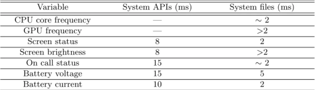
The operating system (OS) generates traces and logs to indicate its current state and the status of the peripherals. Thus, instead of encumbering the system with queries for the values of the inputs, the system files are read in parallel. Data from experimentation also showed that it is also faster to read the system files than to use system APIs (Table 3).
Table 3: The mean time needed to access the value of some variables through Android APIs and through system files, on the smartphone.
Variable System APIs (ms) System files (ms)
CPU core frequency — ∼ 2
GPU frequency — >2 Screen status 8 2 Screen brightness 8 >2 On call status 15 ∼ 2 Battery voltage 15 5 Battery current 10 2
An application was constructed to read and organize the necessary data. In order to have a correct correlation between the inputs and output, the application reads the data concurrently to minimize the reading time. It divides the reading queries into two halves and lunches two threads. Each of the threads reads the current time and then proceeds to get the readings from the systems files. Once the reading is finished, each of the threads queries for the time again and add it to the end of the data array (Figure 5).
To ensure the sanity of the data, the application compares the starting time of each of the threads and its ending time (TS3 - TS1 and TS4 - TS2). Then, it compares the start of the thread that started first
TS1 R(1) R(2) … R(n/2) TS3
TS2 R(n/2 +1) R(n/2 +2) … R(n) TS4
Figure 5: Concurrent readings (R) of n pieces of data with timestamps (TS).
with the end of the second one, to compute the time of the whole process. The process should not take more than 20 ms (the average is around 10 ms), with each thread taking at most 10 ms. Otherwise, the data is considered corrupted and discarded.
The choice of 10 ms for each thread is based on the time the Linux Kernel gives to each process before pausing it and changing to another (Multitasking). The 20 ms limit is imposed to be able to follow the fastest-changing variable, i.e. the CPU frequency [90]. Hence, the sampling time is 20 ms to follow this variable. T S3 − T S1 ≤ 10 ms T S4 − T S2 ≤ 10 ms T S4 − T S1 ≤ Ts, Ts= 20 ms (4)
To keep the model as simple as possible—and consequently as computationally optimized as possible, only the most characterizing and directly influential inputs for each of the components were included. 4.4. The choice of inputs
• The SoC
CPU power consumption is a function of its frequency and voltage [44]. Moreover, the voltage in processors with dynamic voltage and frequency scaling (DVFS) is also a function of the frequency [19]. Thus, the input used to estimate power consumption is the frequency f of each CPU core. However, the CPU on the smart-phone was configured to use one frequency for each of the quad-core blocks in its big.Little configuration. Therefore, there will only be two frequency readings for that device [91]. The same input—the frequency—is used for the GPU since it correlates directly with its power consumption [32].
• The RAM
The RAM consumes around 10% of the total system power [92]. To account for the power used by the RAM, in the first trials, the value of the occupied RAM was used as an input characterizing the power draw of the RAM. However, that value on its own does not factor the maximum and the minimum possible values of the RAM on the system. Henceforth, the ratio of the occupied RAM over its maximum value is used and called the Memory Occupation Rate (MOR).
• The communication peripherals
The communication peripherals are the phone’s LTE module, the wireless chip (Wi-Fi and Bluetooth), and the GPS. Power consumption for these peripherals is mostly characterized by their state of connection and data transfer [52, 83]. For the LTE chip, the inputs are the On-call status (Off, 2G, 3G, LTE), the signal strength, and the connection and data transfer mode. Similarly, for the Wi-Fi and Bluetooth, as their power consumption is heavily influenced by their state of activity and the bandwidth [70], the inputs are the status (On/Off) and the data transfer. Finally, for the GPS, only the status was used.
To account for the power draw of the touchscreen, the status of the screen (On/Off) and its brightness are used as inputs [80, 89], since for modern AMOLED screens, consumed power is a quadratic function of the brightness [89, 52]. The power consumed by the screen is also dependent on the used resolution and scaling [11]. However, since in the case of this work, the resolution will be fixed to the maximum possible value without any scaling, it will be a constant that won’t affect the model.
For the speakers, the status (On/Off) and the volume are used as inputs for the model [81]. As for the microphone, only the status was used. Finally, for the cameras and the LED flashlight, the status of the camera its recording status (Camera recording or not) alongside the flash (On/Off) are used.
4.5. The modeling scheme
Microprocessors-based SoCs are very complex and contain a large number of sub-modules. White-box techniques would require the modeling of all those components, making the process of constructing one arduous [25, 42].
The availability of the traces provided by the OS, alongside the complexity of the system, leads us towards the use of black-box modeling techniques. In this modeling scheme, there is a choice between either regression-based identification techniques or correlation and classification ones. Regression-based power models have been thoroughly studied in the literature [28, 29, 80, 32, 20, 55], especially for smartphones. Nevertheless, their accuracy was undermined by the fact that most of them used linear-regression, which led to an increased estimation error when the power dynamics were not as linear.
Nonlinear models like artificial neural networks (ANN) avoid these shortcomings [19, 51, 66]. However, Classic ANN do not account for the sampling time or the different timestamps associated with data. They are also not built to account for feedback loops, where previous values of the output influence the value of the next output. One alternative was recently explored by Romansky et al. [54] who used times series and deep learning to predict energy consumption in their model Deep Green.
The solution implemented in this work is the Nonlinear Autoregressive Network with eXogenous inputs (NARX) neural networks. These networks are recursive neural networks build to predict the output of time series [93]. Equation 5 gives their mathematical representation.
y(k) = ϕ [y(k − 1), · · · , y(k − dy), u(k − n), u(k − n − 1), · · · , u(k − n − du)] (5)
y(k) and u(k) are the output to be predicted and the input at the time step k, respectively. ϕ is the characteristic function. The term n is the process dead-time, whereas dy and du are the orders of time
delays for the input and output, also called input and output memory. Since the power changes react pretty quickly with changes in the characteristics (inputs), dy, du, and n were all set to the value of 1, giving:
y(k) = ϕ [y(k − 1), y(k − 2), u(k − 1), u(k − 2)] (6)
The NARX model is composed of two layers: a hidden layer and an output layer. The neurons in the hidden layer have sigmoids (ς) as activation functions. The output layer contains a single neuron, representing the total consumed power by the device PSystem, with a linear transfer function (Figure 6).
The first advantage of using these neural networks is their capacity to estimate nonlinear dynamics while still keeping a relatively simple and computationally light form (2-layers). The second advantage is the component-level granularity.
To illustrate the capacity of the model to reach this level of granularity, Figure 7 describes the distribution of the total power consumed by a typical device as the sum of the power consumed by each individual component (CPU, Wi-Fi, ...), plus a minimum amount of base still consumed by the device [80], and a negligible amount consumed by the rest of the components whose consumption is marginal (see 4.1). Assuming that the power consumed the components whose consummation is marginal and the base power represents a single static power, the power consumed by the device becomes:
PT otal= PStatic+ n
X
i=1
y(k) u(k) z-1 f 1(u(k), u(k -1)) z-1 f 2(y(k), y(k -1)) Σ 𝜑(y(k), … ,y(k -1) u(k), …, u(k -1))
Figure 6: The general structure of N3 NARX model.
Where i denotes the component number (CPU, GPU, RAM...), and n is the total number of these compo-nents. The power consumed by each of these components can be correlated with one of its characteristics. These characteristics will be used as inputs to the power model.
The level of granularity can be ensured by configuring the neurons of the hidden layer so as to achieve component decoupling, by disabling the training of the weights w linking the neurons of the different com-ponents. Figure 8 shows the configuration of the power model for an embedded system and showcases the interconnection of the neurons related to three components: the SoC, Camera 1 and the screen. Since the output layer is a linear neuron, the power consumed by the system becomes:
PSystem= w1ς1+ · · · + wnςn+ wn+1ςn+1+ wn+2ςn+2+ · · · +
wmςm+ wm+1ςm+1+ wm+2ςm+2+ · · · + wjςj+ wj+1ςj+1+ wiςi (8)
by disabling all the components except the SoC, as this is the component required for system operation, and training the model with data from this configuration, the power consumption of the system becomes (from Equation 7):
PSyst`eme= PStatique+ PSoC (9)
whereas for the NARX model (Equation 8), this translates into:
PSyst`eme= w1ς1+ · · · + wnςn+ wn+1ςn+1+ wn+2ςn+2+ wiςi
| {z }
PStatique+ PSoC
(10)
In order to quantify the individual contribution of each component, the training set is constructed as follows. At first, only the SoC is active for a period of time. Then the components are activated one after the other. Each component is kept active for a duration of time, after which it is deactivated for a period of time before activating the next component. Finally, All the components are returned to their automatic operating state.
Thus, the NARX model gives estimates of the power consumed by the system as a whole, as well as the
Figures/Power_Consumption_Destribution-eps-converted-to.pdf
𝜍1 𝑧−1 𝜍𝑗 𝑧−1 𝑔 𝑓1 𝑆𝑡𝑎𝑡𝑢𝑠𝑂𝑛/𝑜𝑓𝑓 𝑃𝑆𝑦𝑠𝑡𝑒𝑚 𝑧−1 𝜍𝑛 𝑧−1 𝑓𝑛 𝜍𝑛+1 𝑧−1 𝑓𝐺𝑃𝑈 𝜍𝑛+2 𝑧−1 𝑀𝑂𝑅 ⋮ 𝜍𝑚 𝑧−1 𝑆𝑡𝑎𝑡𝑢𝑠𝑂𝑛/𝑂𝑓𝑓 𝜍𝑚+1 𝑧−1 𝑅𝑒𝑐𝑜𝑟𝑑𝑖𝑛𝑔 𝜍𝑚+2 𝑧−1 𝐹𝑙𝑎𝑠ℎ ⋮ ⋮ 𝑆𝑜𝐶 𝐶𝑎𝑚𝑒𝑟𝑎1 𝑤1 𝑤2 𝑤𝑛+1 𝑤𝑛+2 𝑤𝑚 𝑤𝑚+1 𝑤𝑚+2 𝜍𝑖 𝜍𝑗+1 𝑧−1 𝑤𝑗+1 𝐵𝑟𝑖𝑔ℎ𝑡𝑛𝑒𝑠𝑠 𝑤 𝑖 𝑤𝑗 𝑆𝑐𝑟𝑒𝑒𝑛 ቐ
Figure 8: The configuration of the interconnections of neurons in the hidden layer in the NARX power model to ensure the components’ level granularity.
power consumed by the components individually:
PSystem= w1ς1+ · · · + wnςn+ wn+1ςn+1+ wn+2ςn+2+ wiςi | {z } PStatique+ PSoC wmςm+ wm+1ςm+1+ wm+2ςm+2 | {z } PCamera1 + · · · + wjςj | {z } PScreen (11)
4.5.1. Model construction and Implementation
NARX neural networks require relatively large amounts of data and resources to be trained into accuracy. Mobile CPU are not yet capable of doing such training. In fact, during experimentation, it took around 45 minutes to train N3 on the device with 8 × 10⁴ data points, and when the number of data points exceeded
1.2 × 10⁵, the device would just shut down.
The evident solution to these limitations is to do the training on a separate device. Therefore, the model construction process would start with data gathering. The data will then be transferred to a separate device to train N3. Once the training process finished, N3will be installed on the profiled device to generate online
estimations. 4.6. Summary
Table 4: Summarized description of the profiler.
Purpose Monitoring
Granularity Components level Source measurement System traces
Device Smartphone Development board
Model name N3
Modelling scheme Neural network
Number of layers 2
• Hidden layer: 26 neurons • Hidden layer: 5 neurons • Output layer: 1 neuron
Inputs SoC • f1: CPU0–3 • f : CPU0 • f2: CPU4–7 • MOR • fGP U • MOR Cellular radio • Connection status: Off/2G/3G/LTE • On-Call status: On/Off • Signal strength (%) • Data transfer mode :
• LTE: idle/DRX/... • 3G: DCH/FACH... • Data transfer rate Wi-Fi • Status: On/Off • Data transfer: 0/1 Bluetooth • Status: On/Off • Data transfer: 0/1 GPS • Status: On/Off Screen
• Status: On/Off • Status: On/Off • Brightness: (%) • Brightness: (%) Speakers • Status: On/Off • Volume: (%) Microphone • Recording: 0/1 Cameras • Status: On/Off • Recording: 0/1 • flashlight: On/Off
Modelling construction Off-device Modelling Implementation On-device
Sampling time 20 ms
5. Experimental results and discussion 5.1. Model training
For the best training results, the gathered data need to cover as much of the usage scenarios as possible. To do so, the experimentation use case covers several standard benchmarks and then typical tasks performed by devices. It goes as follows. Firstly, a set of benchmarks is launched successively: AnTuTu [94], Geekbench
Table 5: The training time needed for different numbers of samples alongside the resulted mean absolute percentage error (MAPE), the mean squared error (MSE), and the regression (R) for the test set.
Smartphone Development board
Total number of
samples
Training
time (min) MAPE (%) MSE R
Training
time (min) MAPE (%) MSE R
∼ 8 × 10⁴ 7 5 7.56 × 10− 3 0.986 4 2.9 4.72 × 10− 3 0.942 ∼ 2 × 10⁵ 12 3 7.23 × 10− 3 0.986 6 2.9 4.68 × 10− 3 0.942 ∼ 4 × 10⁵ 14 2.9 7.18 × 10− 3 0.986 10 2.8 3.67 × 10− 3 0.942 ∼ 8 × 10⁵ 20 2.4 7.60 × 10− 4 0.987 12 2.8 3.56 × 10− 3 0.963 ∼ 1.2 × 10⁶ 32 2.2 7.48 × 10− 4 0.987 15 2.8 3.61 × 10− 3 0.961 ∼ 1.8 × 10⁶ 57 2.2 7.09 × 10− 4 0.987 19 2.8 3.54 × 10− 3 0.961
4 [95], PCMark [96], and 3DMark [97]. These benchmarks are used to test the maximum performance of the systems through multiple calculation tests, 3D renderings... The successive launch of these benchmarks would generate data describing the system under heavy workloads. It would also stress the system and account for its behavior under thermal throttling (if present).
Then, the system—when appropriate, as the development board lacks multimedia and communication functionality—is put through more common tasks: A phone call, an internet video call, local video playback, video streaming, audio playback, file download over the cellular network, then over Wi-Fi, taking a picture without flash, with flash, and recording a 30 s video, and finally leaving the phone idle for a while. This data-gathering experiment is repeated multiple times with variations in the order of the benchmarks as well as the tasks.
The gathered data is then divided into three sets: a training set (60%), and a validation set (20%) to train the model, and a test set (20%) to evaluate its performance. The results of the test sets for different sizes of training sets are shown in Table 5. These results demonstrate how the inputs correlate with the output (R ≈ 1). Moreover, the predictions fit the output, with very low errors (MAPE = 2.2% for the smartphone and 2.8% for the board), indicating the accuracy of the model. Thus, N3 is validated.
Nevertheless, Table 5 also shows the limitations of using neural networks. Indeed, the MAPE went down from 5% to 2.2% by adding more samples, but it came at the cost of longer training times. Additionally, after a certain number of samples (1.8 × 10⁶for the smartphone and 2 × 10⁵), the MAPE no longer improved.
5.2. Real-time usage validation
In the model construction process, the profiler was set to generate estimations online. Having validated the model through the test sets, it is, then, incorporated alongside the data logging program into the ap-plication and directly deployed onto the device. Then, its accuracy and performance are tested through a non-scripted randomized normal usage of the device. This test, which is set to mimic day-to-day activities, includes making cellular and video calls through applications, sending messages through SMS and applica-tions services (Smartphone only), video playback and streaming, taking and sending pictures (Smartphone only), browsing the web, and finally playing two different games (Smartphone only).
Table 6 highlights the online performance of the model on both devices, while in figure 9 and figure 11, the measured power consumption of the smartphone is drawn against values estimated by N3 for the smartphone and the development board, respectively. For the smartphone, the model accurately predicts the power consumed by the phone with minimal estimation errors. It has an estimation MAPE of only 2.82%, and the recorded Mean Absolute Error (MAE) is 0.0168 W, whereas the Mean Squared Error (MSE) is 7.04 × 10⁻⁴. Moreover, 97% of the estimation sample made by the model had an error value of zero
(or less than the precision of the measurements which is 10−3). Furthermore, the errors are normally distributed for both devices (verified by K-S test, Figure 10). For the smartphone, the estimation errors had a mean µε= 1, 178 × 10−4W and standard deviation σε= 0, 0265. Whereas for the development board,
µε= 0.0116W and σε= 0, 037. Both residuals present no heteroskedasticity (Engle’s ARCH test).
Finally, on the development board, as can be seen in figure 11, the estimations had a delay (of about 0.2 s). This delay is a result of the wait time needed by the board to receive the measurements from the external multimeter to the device. Once accounted for this delay, the model performance results were practically the same as they were on the smartphone.
Table 6: Online testings results of the model on both devices. Smartphone Development board Test Duration 2.25 h 1.5 h Number of Samples ∼ 403 × 103 ∼ 280 × 103 MAE (W) 0.0168 0.038 MAPE (%) 2.82 2.88 MSE 7.04 × 10⁻⁴ 5.74 × 10⁻³ Perfect fits (%) 97 96.6 Figures/PowerModel_A-eps-converted-to.pdf
Figure 9: Online N3 Power estimation against the measurements for the smartphone.
Figures/PowerModel_A_Error_Values-eps-converted-to.pdf
Figure 10: N3 Online estimation error distribution for the smartphone.
5.3. Performance evaluation and comparison
Performance-wise, the average sampling time was 19.8 ms which satisfies the previously stated design constraint. Additionally, N3 caused no issues or bottlenecks for the system, as indicated by its overhead. The overhead is computed by running the system with the profiler and then comparing its power consumption and load to data from instances that had no profiling [37]. N3 it had only a 3% load overhead during the test. As for the power overhead, it only amounted to a 5% increase in the same test.
Finally, we compared the results of N3 with the publicly available power models and models of which the MAPE was reported in the literature. Table 7 shows the accuracy of these models compared to the power model presented in this paper.
While we are pleased that our model performed better than or on par with established works, it is also worth noting that some of these profilers have higher levels of granularity than our model does. Furthermore, some works, like PowerBooter, have not been updated for several years.
6. Conclusion
Given the great importance of estimating power consumption in embedded systems and smartphones, the literature has seen a great deal of research devoted to this subject. In this paper, we have presented, through an in-depth study of the literature, a generic methodology for building power profilers by adapting the profiling process to their context of use. The method is streamlined into a set of manageable steps, explaining the design choices to be made through each of them, starting with the goal of building the profiler. Then, we presented a compilation of profilers and models found in the literature and categorized them according to the steps explained in the proposed methodology.
Figures/PowerModel_DB-eps-converted-to.pdf
Figure 11: Online N3Power estimation against the measurements for the development board.
Table 7: Comparison of the accuracy of several power models and profilers.
Profiler / Model MAPE (%) Source Year N3 2.88 Measured 2019 Snapdragon Profiler 4.8 Measured 2018 Trepn 5.5 Measured 2018 Yoon et al. [31] 5.1 [31] 2017 PETrA 4 [33] 2017 Walker et al. [35] 3.8 [35] 2017 Djedidi et al. [19] 4.4 [19] 2017 Kim et al. [32] 2.9 [32] 2015 eLens ∼ 10 [77] 2013 Kim et al. [80] 3.8 ∼ 7.2 [80] 2012 Power Doctor 10 [74] 2012 eProf 10 [74] 2011 Sesame 5 [29] 2011 PowerBooter 4.1 / 24 [28]/Measured 2010/2018
The proposed methodology is then applied in this work to build a new accurate profiler, based on a NARX neural network model, and used as a monitoring tool to detect anomalies in power consumption. In the results section, the proposed model has been implemented and validated with outstanding results—best in its class—that highlight how the accuracy reported in the literature is improved while maintaining low power and computational overhead.
Thus, N3 is a profiler capable of generating accurate online power estimation for mobile and embedded
devices, making it the optimal tool for power monitoring and debugging, and using the power profile to detect anomalies in the system. Finally, thanks to its accuracy and performance, N3 has been implemented
in an online monitoring framework for safety-critical avionic systems [18].
[1] M. A. Hoque, M. Siekkinen, K. N. Khan, Y. Xiao, S. Tarkoma, Modeling, Profiling, and Debugging the Energy Consump-tion of Mobile Devices, ACM Computing Surveys 48 (3) (2015) 1–40, ISSN 03600300, doi:10.1145/2840723.
[2] J.-M. Kang, C.-K. Park, S.-S. Seo, M.-J. Choi, J. W.-K. Hong, User-Centric Prediction for Battery Lifetime of Mobile Devices, in: CHALLENGES FOR NEXT GENERATION NETWORK OPERATIONS AND SERVICE MANAGEMENT, PROCEEDINGS, vol. 5297, Springer, Berlin, Heidelberg, ISBN 978-3-540-88622-8, ISSN 0302-9743, 531–534, doi:10.1007/ 978-3-540-88623-5 69, 2008.
[3] D. Kim, Y. Chon, W. Jung, Y. Kim, H. Cha, Accurate Prediction of Available Battery Time for Mobile Applications, ACM Transactions on Embedded Computing Systems 15 (3) (2016) 1–17, ISSN 15399087, doi:10.1145/2875423. [4] A. Kanduri, M. H. Haghbayan, A. M. Rahmani, P. Liljeberg, A. Jantsch, H. Tenhunen, N. Dutt, Accuracy-Aware Power
Management for Many-Core Systems Running Error-Resilient Applications, IEEE Transactions on Very Large Scale Inte-gration (VLSI) Systems 25 (10) (2017) 2749–2762, ISSN 10638210, doi:10.1109/TVLSI.2017.2694388.
[5] B. Martinez, M. Mont´on, I. Vilajosana, J. D. Prades, The Power of Models: Modeling Power Consumption for IoT Devices, IEEE Sensors Journal 15 (10) (2015) 5777–5789, ISSN 1530437X, doi:10.1109/JSEN.2015.2445094.
[6] M. A. Bokhari, B. Alexander, M. Wagner, In-vivo and offline optimisation of energy use in the presence of small en-ergy signals, in: Proceedings of the 15th EAI International Conference on Mobile and Ubiquitous Systems: Computing, Networking and Services - MobiQuitous ’18, ACM Press, New York, New York, USA, ISBN 9781450360937, 207–215, doi:10.1145/3286978.3287014, 2018.
[7] E. Demirbilek, J.-C. Grgoire, A. Vakili, L. Reyero, Modelling and improving the battery performance of a mobile phone application: A methodology, in: 5th International Conference on Energy Aware Computing Systems and Applications, ICEAC 2015, IEEE, ISBN 9781479917716, 1–4, doi:10.1109/ICEAC.2015.7352165, 2015.
[8] J. M. Kim, Y. G. Kim, S. W. Chung, Stabilizing CPU frequency and voltage for temperature-aware DVFS in mobile devices, IEEE Transactions on Computers 64 (1) (2015) 286–292, ISSN 00189340, doi:10.1109/TC.2013.188.
[9] J. G. Park, C. Y. Hsieh, N. Dutt, S. S. Lim, Quality-aware mobile graphics workload characterization for energy-efficient DVFS design, in: 2014 IEEE 12th Symposium on Embedded Systems for Real-Time Multimedia, ESTIMedia 2014, IEEE, ISBN 9781479963072, 70–79, doi:10.1109/ESTIMedia.2014.6962347, 2014.
[10] S. Li, S. Mishra, Optimizing power consumption in multicore smartphones, Journal of Parallel and Distributed Computing 95 (2015) 124–137, ISSN 07437315, doi:10.1016/j.jpdc.2016.02.004.
[11] M. Linares-V´asquez, G. Bavota, C. E. B. C´ardenas, R. Oliveto, M. Di Penta, D. Poshyvanyk, Optimizing energy consump-tion of GUIs in Android apps: a multi-objective approach, in: Proceedings of the 2015 10th Joint Meeting on Foundaconsump-tions of Software Engineering - ESEC/FSE 2015, ACM Press, New York, New York, USA, ISBN 9781450336758, 143–154, doi:10.1145/2786805.2786847, 2015.
[12] Y. Guo, C. Wang, X. Chen, Understanding application-battery interactions on smartphones: A large-scale empirical study, IEEE Access 5 (2017) 13387–13400, ISSN 21693536, doi:10.1109/ACCESS.2017.2728620.
[13] A. M. Abbasi, M. Al-tekreeti, Y. Ali, K. Naik, A. Nayak, N. Goel, B. Plourde, A framework for detecting energy bugs in smartphones, in: 2015 6th International Conference on the Network of the Future (NOF), IEEE, ISBN 978-1-4673-8386-8, 1–3, doi:10.1109/NOF.2015.7333297, 2015.
[14] J. Koo, K. Lee, W. Lee, Y. Park, S. Choi, BattTracker: Enabling energy awareness for smartphone using Li-ion battery characteristics, in: Proceedings - IEEE INFOCOM, vol. 2016-July, IEEE, ISBN 9781467399531, ISSN 0743166X, 1–9, doi:10.1109/INFOCOM.2016.7524422, 2016.
[15] L. Caviglione, M. Gaggero, J. F. Lalande, W. Mazurczyk, M. Urba´nski, Seeing the unseen: Revealing mobile malware hidden communications via energy consumption and artificial intelligence, IEEE Transactions on Information Forensics and Security 11 (4) (2016) 799–810, ISSN 15566013, doi:10.1109/TIFS.2015.2510825.
[16] A. Merlo, M. Migliardi, P. Fontanelli, Measuring and estimating power consumption in Android to support energy-based intrusion detection, Journal of Computer Security 23 (5) (2015) 611–637, ISSN 0926227X, doi:10.3233/JCS-150530. [17] G. Suarez-Tangil, J. E. Tapiador, P. Peris-Lopez, S. Pastrana, Power-aware anomaly detection in smartphones: An analysis
of on-platform versus externalized operation, Pervasive and Mobile Computing 18 (2015) 137–151, ISSN 15741192, doi: 10.1016/j.pmcj.2014.10.007.
[18] O. Djedidi, M. A. Djeziri, N. K. M’Sirdi, Data-Driven Approach for Feature Drift Detection in Embedded Electronic Devices, IFAC-PapersOnLine 51 (24) (2018) 1024–1029, ISSN 24058963, doi:10.1016/j.ifacol.2018.09.714.
[19] O. Djedidi, M. A. Djeziri, N. K. M’Sirdi, A. Naamane, Modular Modelling of an Embedded Mobile CPU-GPU Chip for Feature Estimation, in: Proceedings of the 14th International Conference on Informatics in Control, Automation and Robotics, vol. 1, SciTePress, Mardrid, Spain, ISBN 978-989-758-263-9, 338–345, doi:10.5220/0006470803380345, 2017. [20] N. K. Shukla, R. Pila, S. Rawat, Utilization-based power consumption profiling in smartphones, in: Proceedings of the
2016 2nd International Conference on Contemporary Computing and Informatics, IC3I 2016, IEEE, ISBN 9781509052554, 881–886, doi:10.1109/IC3I.2016.7919046, 2016.
[21] E. Rattagan, E. T. Chu, Y. D. Lin, Y. C. Lai, Semi-online power estimation for smartphone hardware components, in: 2015 10th IEEE International Symposium on Industrial Embedded Systems, SIES 2015 - Proceedings, IEEE, ISBN 9781467377119, 174–177, doi:10.1109/SIES.2015.7185058, 2015.
[22] R. Mittal, A. Kansal, R. Chandra, Empowering developers to estimate app energy consumption, in: Proceedings of the 18th annual international conference on Mobile computing and networking - Mobicom ’12, ACM Press, New York, New York, USA, ISBN 9781450311595, 317, doi:10.1145/2348543.2348583, 2012.
[23] J. Huang, R. Li, J. An, D. Ntalasha, F. Yang, K. Li, Energy-Efficient Resource Utilization for Heterogeneous Embedded Computing Systems, IEEE Transactions on Computers 66 (9) (2017) 1518–1531, ISSN 00189340, doi:10.1109/TC.2017. 2693186.
[24] L. Niu, D. Zhu, Reliability-aware scheduling for reducing system-wide energy consumption for weakly hard real-time systems, Journal of Systems Architecture 78 (2017) 30–54, ISSN 1383-7621, doi:10.1016/J.SYSARC.2017.06.004. [25] R. W. Ahmad, A. Gani, S. H. A. Hamid, F. Xia, M. Shiraz, A Review on mobile application energy profiling: Taxonomy,
state-of-the-art, and open research issues, Journal of Network and Computer Applications 58 (2015) 42–59, ISSN 10958592, doi:10.1016/j.jnca.2015.09.002.
[26] E. Benkhelifa, T. Welsh, L. Tawalbeh, Y. Jararweh, A. Basalamah, Energy Optimisation for Mobile Device Power Con-sumption: A Survey and a Unified View of Modelling for a Comprehensive Network Simulation, Mobile Networks and Applications 21 (4) (2016) 575–588, ISSN 15728153, doi:10.1007/s11036-016-0756-y.
[27] I. Qualcomm Innovation Center, Trepn Profiler - Android Apps on Google Play, URL https://play.google.com/store/ apps/details?id=com.quicinc.trepn&hl=fr CH, 2019.
[28] L. Zhang, B. Tiwana, Z. Qian, Z. Wang, R. P. Dick, Z. M. Mao, L. Yang, Accurate online power estimation and auto-matic battery behavior based power model generation for smartphones, in: Proceedings of the eighth IEEE/ACM/IFIP international conference on Hardware/software codesign and system synthesis - CODES/ISSS ’10, ACM Press, New York, New York, USA, ISBN 9781605589053, 105, doi:10.1145/1878961.1878982, 2010.
[29] M. Dong, L. Zhong, Self-constructive high-rate system energy modeling for battery-powered mobile systems, in: MobiSys, ACM Press, New York, New York, USA, ISBN 9781450306430, ISSN 10769757, 335, doi:10.1145/1999995.2000027, 2011. [30] L. Ardito, G. Procaccianti, M. Torchiano, G. Migliore, Profiling Power Consumption on Mobile Devices, in: Proceedings of The Third International Conference on Smart Grids, Green Communications and IT Energy-aware Technologies, IARIA, Lisbon, 101–106, 2013.
[31] C. Yoon, S. Lee, Y. Choi, R. Ha, H. Cha, Accurate power modeling of modern mobile application processors, Journal of Systems Architecture 81 (2017) 17–31, ISSN 13837621, doi:10.1016/j.sysarc.2017.10.001.
[32] Y. G. Kim, M. Kim, J. M. Kim, M. Sung, S. W. Chung, A novel GPU power model for accurate smartphone power breakdown, ETRI Journal 37 (1) (2015) 157–164, ISSN 22337326, doi:10.4218/etrij.15.0113.1411.
[33] D. Di Nucci, F. Palomba, A. Prota, A. Panichella, A. Zaidman, A. De Lucia, PETrA: A Software-Based Tool for Estimating the Energy Profile of Android Applications, in: 2017 IEEE/ACM 39th International Conference on Software Engineering Companion (ICSE-C), IEEE, ISBN 978-1-5386-1589-8, 3–6, doi:10.1109/ICSE-C.2017.18, 2017.
[34] S. A. Chowdhury, A. Hindle, GreenOracle: Estimating Software Energy Consumption with Energy Measurement Corpora, in: Proceedings of the 13th International Workshop on Mining Software Repositories - MSR ’16, ACM Press, New York, New York, USA, ISBN 9781450341868, 49–60, doi:10.1145/2901739.2901763, 2016.
[35] M. J. Walker, S. Diestelhorst, A. Hansson, A. K. Das, S. Yang, B. M. Al-Hashimi, G. V. Merrett, Accurate and Stable Run-Time Power Modeling for Mobile and Embedded CPUs, IEEE Transactions on Computer-Aided Design of Integrated Circuits and Systems 36 (1) (2017) 106–119, ISSN 02780070, doi:10.1109/TCAD.2016.2562920.
[36] K. Kim, D. Shin, Q. Xie, Y. Wang, M. Pedram, N. Chang, FEPMA: Fine-Grained Event-Driven Power Meter for Android Smartphones Based on Device Driver Layer Event Monitoring, in: Design, Automation I& Test in Europe Conference and Exhibition (DATE), IEEE Conference Publications, New Jersey, ISBN 9783981537024, ISSN 15301591, 1–6, doi: 10.7873/DATE.2014.380, 2014.
[37] A. Dzhagaryan, A. Milenkovi´c, M. Milosevic, E. Jovanov, An Environment for Automated Measuring of Energy Consumed by Android Mobile Devices, in: PECCS 2016 - Proceedings of the 6th International Joint Conference on Pervasive and Embedded Computing and Communication Systems, SCITEPRESS - Science and Technology Publications, Lisbon, Portugal, ISBN 978-989-758-195-3, 28–39, doi:10.5220/0005950800280039, 2016.
[38] L. Sun, R. K. Sheshadri, W. Zheng, D. Koutsonikolas, Modeling WiFi active power/energy consumption in smartphones, in: Proceedings - International Conference on Distributed Computing Systems, IEEE, ISBN 9781479951680, ISSN 1063-6927, 41–51, doi:10.1109/ICDCS.2014.13, 2014.
[39] O. Djedidi, M. A. Djeziri, N. K. M’Sirdi, A. Naamane, A Novel Easy-to-construct Power Model for Embedded and Mobile Systems Using Recursive Neural Nets to Estimate Power Consumption of ARM-based Embedded Systems and Mobile De-vices, in: Proceedings of the 15th International Conference on Informatics in Control, Automation and Robotics (ICINCO 2018), vol. 1, INSTICC, SciTePress, Porto, Portugal, ISBN 978-989-758-321-6, 541–545, doi:10.5220/0006915805410545, 2018.
[40] R. W. Ahmad, A. Gani, S. H. Ab Hamid, A. Naveed, K. O. Kwangman, J. J. Rodrigues, A case and framework for code analysis–based smartphone application energy estimation, International Journal of Communication Systems 30 (10) (2017) e3235, ISSN 10991131, doi:10.1002/dac.3235.
[41] D. Di Nucci, F. Palomba, A. Prota, A. Panichella, A. Zaidman, A. De Lucia, Software-based energy profiling of Android apps: Simple, efficient and reliable?, in: SANER 2017 - 24th IEEE International Conference on Software Analysis, Evolution, and Reengineering, vol. 15, IEEE, ISBN 9781509055012, ISSN 15399087, 103–114, doi:10.1109/SANER.2017. 7884613, 2017.
[42] A. Pathak, Y. C. Hu, M. Zhang, Where is the Energy Spent Inside My App?: Fine Grained Energy Accounting on Smartphones with Eprof, in: Proceedings of the 7th ACM European Conference on Computer Systems, EuroSys ’12, ACM, New York, NY, USA, ISBN 978-1-4503-1223-3, ISSN 15361268, 29–42, doi:10.1145/2168836.2168841, 2012. [43] P. Holleis, M. Luther, G. Broll, B. Souville, A DIY Power Monitor to Compare Mobile Energy Consumption in Situ,
Proceedings of the 15th international conference on Human-computer interaction with mobile devices and services, ACM (2013) 416–421doi:10.1145/2493190.2494087.
[44] M. L. Altamimi, K. Naik, A Computing Profiling Procedure for Mobile Developers to Estimate Energy Cost, in: Proceedings of the 18th ACM International Conference on Modeling, Analysis and Simulation of Wireless and Mobile Systems -MSWiM ’15, ACM Press, New York, New York, USA, ISBN 9781450337625, 301–305, doi:10.1145/2811587.2811627, 2015. [45] A. Pathak, Y. C. Hu, M. Zhang, P. Bahl, Y.-M. Wang, Fine-Grained Power Modeling for Smartphones Using System Call Tracing, in: Proceedings of the sixth conference on Computer systems EuroSys 11, ISBN 9781450306348, 153, doi: 10.1145/1966445.1966460, 2011.
[46] M. J. Dousti, M. Ghasemi-Gol, M. Nazemi, M. Pedram, ThermTap: An online power analyzer and thermal simulator for Android devices, in: Proceedings of the International Symposium on Low Power Electronics and Design, vol. 2015-Septe, IEEE, ISBN 9781467380096, ISSN 15334678, 341–346, doi:10.1109/ISLPED.2015.7273537, 2015.
[47] Y. Fu, L. Li, K. Wang, C. Zhang, Kalman Predictor-Based Proactive Dynamic Thermal Management for 3-D NoC Systems with Noisy Thermal Sensors, IEEE Transactions on Computer-Aided Design of Integrated Circuits and Systems 36 (11) (2017) 1869–1882, ISSN 02780070, doi:10.1109/TCAD..2661808.
[48] N. Zhang, P. Ramanathan, K.-H. Kim, S. Banerjee, PowerVisor: A Battery Virtualization Scheme for Smartphones, in: Proceedings of the third ACM workshop on Mobile cloud computing and services - MCS ’12, ACM Press, New York, New York, USA, ISBN 9781450313193, 37, doi:10.1145/2307849.2307859, 2012.
[49] J. Bornholt, T. Mytkowicz, K. S. McKinley, The model is not enough: Understanding energy consumption in mobile devices, in: 2012 IEEE Hot Chips 24 Symposium (HCS), IEEE, ISBN 978-1-4673-8879-5, 1–3, doi:10.1109/HOTCHIPS. 2012.7476509, URL http://ieeexplore.ieee.org/document/7476509/, 2012.
[50] O. Djedidi, M. A. Djeziri, N. K. M’Sirdi, A. Naamane, Constructing an Accurate and a High-Performance Power Profiler for Embedded Systems and Smartphones, in: Proceedings of the 21st ACM International Conference on Modelling, Analysis and Simulation of Wireless and Mobile Systems (MSWIM ’18), vol. 18, ACM Press, Montr´eal, Canada, ISBN 9781450359603, 79–82, doi:10.1145/3242102.3242139, 2018.
[51] S. Alawnah, A. Sagahyroon, Modeling of smartphones’ power using neural networks, Eurasip Journal on Embedded Systems 2017 (1) (2017) 22, ISSN 16873963, doi:10.1186/s13639-017-0070-1.


![Table 2: Highlights of the specifications of the smartphone and the development boards used in this study [85, 86]](https://thumb-eu.123doks.com/thumbv2/123doknet/14618795.733496/11.892.150.741.215.641/table-highlights-specifications-smartphone-development-boards-used-study.webp)