Iceberg evolution modelling : A background study

Publisher’s version / Version de l'éditeur:

PERD/CHC Report, OERC Report, 2000-05-06

READ THESE TERMS AND CONDITIONS CAREFULLY BEFORE USING THIS WEBSITE. https://nrc-publications.canada.ca/eng/copyright

Vous avez des questions? Nous pouvons vous aider. Pour communiquer directement avec un auteur, consultez la première page de la revue dans laquelle son article a été publié afin de trouver ses coordonnées. Si vous n’arrivez pas à les repérer, communiquez avec nous à [email protected].

Questions? Contact the NRC Publications Archive team at

[email protected]. If you wish to email the authors directly, please see the first page of the publication for their contact information.

Archives des publications du CNRC

For the publisher’s version, please access the DOI link below./ Pour consulter la version de l’éditeur, utilisez le lien DOI ci-dessous.

https://doi.org/10.4224/12341002

Access and use of this website and the material on it are subject to the Terms and Conditions set forth at Iceberg evolution modelling : A background study

Veitch, Brian; Daley, Claude

https://publications-cnrc.canada.ca/fra/droits

L’accès à ce site Web et l’utilisation de son contenu sont assujettis aux conditions présentées dans le site LISEZ CES CONDITIONS ATTENTIVEMENT AVANT D’UTILISER CE SITE WEB.

NRC Publications Record / Notice d'Archives des publications de CNRC: https://nrc-publications.canada.ca/eng/view/object/?id=4995d5c2-329b-4b3d-89f6-46aaac49bdbd https://publications-cnrc.canada.ca/fra/voir/objet/?id=4995d5c2-329b-4b3d-89f6-46aaac49bdbd

Prepared for

National Research Council of Canada By

Brian Veitch and Claude Daley

Faculty of Engineering and Applied Science Memorial University of Newfoundland

May 6, 2000 St. John’s, NF, A1B 3X5 Canada

I

I

c

c

e

e

b

b

e

e

r

r

g

g

E

E

v

v

o

o

l

l

u

u

t

t

i

i

o

o

n

n

M

M

o

o

d

d

e

e

l

l

i

i

n

n

g

g

A

A

B

B

a

a

c

c

k

k

g

g

r

r

o

o

u

u

n

n

d

d

S

S

t

t

u

u

d

d

y

y

TABLE OF CONTENTS

Symbols

Acknowledgement

1 INTRODUCTION ...1

2 DESCRIPTION OF ICEBERGS...2

2.1 Formation of glacial and iceberg ice ...2

2.1.1 Thermodynamic parameters...4 2.1.2 Iceberg calving ...6 2.1.3 Iceberg statistics...8 2.2 Iceberg drift...11 3 ICEBERG EVOLUTION...14 3.1 Ablation Processes...14 3.2 Thermodynamic processes...16 3.2.1 Solar radiation ...16

3.2.2 Forced convection (wind and water) ...16

3.2.3 Buoyant convection ...17

3.2.4 Wave erosion...19

3.3 Fragmentation Processes...21

3.3.1 Global cracking...21

3.3.2 Time dependent strength...23

3.3.3 Thermal cracking ...25

3.4 Deterioration models ...26

3.5 Iceberg shape...29

3.5.1 Shape definition ...31

3.5.2 Coordinate system transformation...32

3.5.3 Hydrostatics and stability ...34

4 MODELING APPROACHES...38

5 CONCLUSIONS ...43

6 REFERENCES ...44

SYMBOLS

a Wave height m

c Specific heat capacity, cohesion J⋅kg-1⋅°C-1, MPa

d Grain size m g Gravitational acceleration m⋅s-2 I Insolation W⋅m-2 k Thermal diffusivity m2⋅s-1 t time s, days K Thermal conductivity W⋅m-1⋅°C-1 Lf Specific latent heat of fusion J⋅kg-1

Lv Specific latent heat of vaporization J⋅kg-1

LWL Waterline length of iceberg m

T Temperature °C

M Mass of the iceberg kg

Nu Nusselt number -

Pr Prandtl number -

qw Heat transfer per unit area W⋅m-2

R melt rate m day-1 Re Reynolds number -

S Surface area, strength m2, MPa

V Volume m3

Vi Horizontal drift velocity m⋅s-1

FB Buoyancy force N

FC Coriolis force N

FDa Air drag force N

FDw Water drag force N

FDi Sea ice indentation force N

FWr Wave radiation force N

FW Weight force N

FP Horizontal pressure gradient force N

α Albedo -

ε& Strain rate s-1

σ Ice strength, stress N⋅m-2

τ Ice shear strength, N⋅m-2

ρi Density of ice kg⋅m-3

ρio Density of pure ice kg⋅m-3

ACKNOWLEDGEMENT

The work was made possible with the support of funding from PERD (Panel on Energy Research and Development). The authors wish to thank Dr. Robert Frederking of the NRC/CHC

1 Introduction

The presence of icebergs poses unique risks to shipping and oil and gas industry operations and subsequently to the ocean environment. These include risks of impact on fixed and floating installations, risks of collision with conventional ship navigation, and risks of scour on sub-sea installations, such as pipelines and wellheads. The consequences of iceberg impact can be severe in terms of the structural integrity of installations, and the safety of personnel and the

environment. This is of immediate concern to the current activities offshore Newfoundland. In assessing iceberg risks, there are several critical components. The population of icebergs is the most important piece of data. Iceberg mass is of similar importance. These two issues have received the most attention to date. However in order to assess specific risks it is necessary to have more data. Shape, movement, and stability are important parameters in modeling the risks due to a collision. Finally, the ice mechanical strength and contact pressures determine the actual interaction effects.

The present work is aimed towards the eventual development of a detailed model of iceberg evolution. While the shape, movement and stability issues are primarily being addressed, iceberg evolution modeling is important to the population, mass and mechanical property issues as well. Icebergs in the Newfoundland and Labrador offshore environment change rapidly as they

migrate from northern latitudes where they originate, to the latitudes around Newfoundland where they disappear. The changes are due to wave erosion and associated calving, natural and forced convective melting, solar radiation melting, and fragmentation due to thermal and motion induced stresses, and reorientation.

The approach taken here is to outline a preliminary model based on a thorough review of the existing state of knowledge of iceberg evolution in terms of thermodynamic decay and

fragmentation. In doing so, the most important physical processes are recognized. Weaknesses in the state of knowledge are identified and an approach for addressing these issues in future is presented. The ultimate aim of the work is to develop a model of the iceberg evolution process that can be used as an experimental tool to improve understanding and to find in these processes the dominant characteristics that can inform iceberg risk assessment. Necessarily, the

2 Description of Icebergs

2.1 Formation of glacial and iceberg ice

Glacial ice is formed from snow. The transition from snow to ice is gradual and depends on temperature and pressure. Warmer temperatures, such as those experienced at temperate glaciers, speed the transition. The process is slower on the colder Polar glaciers. The transition from snow to ice occurs when air pockets within and between grains no longer connect, which occurs at a density of about 830 kg⋅m-3. As the density of pure ice is about 917 kg⋅m-3, air bubbles can make up to about 10% of the volume of ice. Further increases in glacial ice density from about 830 kg⋅m-3 requires that the air bubbles, which are typically on the order of a tenth of a millimeter in diameter, be compressed. Depths at which the ice transition has been measured are variable, but 50m to 90m are typical. Densities for types of snow and ice are given in Table 1. Glacial ice crystals tend to be randomly oriented and are typically 1 to 4 mm across, although they can be considerably larger. Paterson (1994, pp.8-25) gives a more comprehensive description of glacial snow and ice.

Table 1. Densities of snow and ice (after Paterson, p.9).

Description ρ

[kg⋅m-3]

New snow - settled snow 50-300

Depth hoar and wind packed snow 100-400

Firn and wet snow 400-830

Glacier ice 830-917

Reported values of porosity from five icebergs grounded along the coast of Newfoundland yield an average density of approximately 893±7 kg⋅m-3 (Gammon et al. 1983). The same measurement program indicated that the iceberg ice contained few impurities and had a mean grain size of about 15mm. Mean crack densities of 0.35/cm and 0.26/cm for two of the icebergs were reported, where crack density is defined as the number of visible cracks per unit length along a straight line. Sources of cracks include glacial origins, thermal stress induced cracks, and cracks from stress due to hydrostatic and dynamic forces.

The authors also reported results of a set of 11 uniaxial compression tests of iceberg ice done at an average of -4.2°C over a narrow range of temperature and an approximately constant strain rate of 1.085×10-3s-1. The mean values of the elastic modulus and uniaxial compressive strength were 6092 MPa and 5.34 MPa, respectively. They did tests with freshwater ice for comparison

and found that iceberg ice was about 35% stronger and tended to be less brittle, which the authors speculated could be due to possible stress diffusing effects of bubbles near crack tips, which may inhibit crack propagation in iceberg ice.

Subsequent laboratory triaxial, uniaxial, and flexural strength experiments that were done over a range of temperatures and strain rates with ice from four icebergs and a glacier indicated that bubbles may have an important effect on uniaxial and flexural strength (Gagnon & Gammon 1995a, 1995b). This laboratory work included detailed measurements of bubbles, crystal

structure, and crack density (a mean of 0.63/cm was measured). Reported values of fractional porosity indicated density values in the range between 886 kg⋅m-3 and 910 kg⋅m-3, with a mean of 895 kg⋅m-3, which is similar to the earlier findings.

There were considerable variations in the results from different ice sources, but some representative results can be shown here to give an indication of the mechanical properties of iceberg ice. For example, results of 24 flexural strength tests done at a strain rate of 10-3s-1 between -1°C and -16°C indicated that the flexural strength Sf depended on temperature

according to 2 00213 . 0 0738 . 0 8827 . 0 T T S_f = − − (1)

so that, for example, the flexural strength at -10°C is 1.41 MPa.

A summary of the results of some of the triaxial tests reported by Gagnon & Gammon 1995b is presented in Table 2. Note that the each of the 20 data sets referred to in column 1 consisted of 5 experiments.

Other laboratory experiments on iceberg ice have been reported by El-Tahan et al. (1984). They did uniaxial, multiaxial, and indentation tests with small test samples at moderately high strain rates meant to reflect their interest in iceberg impact loads.

Another physical characteristic of glacial ice and icebergs is the presence of large cracks and other defects, such as firn covered crevasses, which can extend for several kilometers in length and be several tens of meters deep (Bader 1977, Kovacs 1977). Crevasses can fill with snow and frost and can eventually transform into ice, or approach the transformation point, but remain weak in tensile strength compared to surrounding ice. In glaciers and tabular icebergs, these flaws tend to be vertical, but not parallel.

Table 2. Triaxial compressive strength (after Gagnon & Gammon 1995b). data set mean strength S standard deviation confining pressure strain rate ε& temperature T

[MPa] [MPa] [MPa] [10-3 s-1] [C]

1 4.43 1.00 0.00 1.45 -1 2 10.29 0.68 1.38 3.93 -1 3 10.17 0.95 3.45 4.34 -1 4 10.74 1.07 6.89 4.84 -1 5 8.67 0.60 13.79 5.13 -1 6 12.27 0.95 1.38 3.76 -6 7 13.22 0.85 6.89 4.73 -6 8 7.82 1.63 0.00 1.63 -11 9 10.75 0.84 1.38 77.50 -11 10 14.64 0.89 1.38 3.46 -11 11 3.50 0.21 1.38 0.0482 -11 12 11.98 1.21 3.45 75.50 -11 13 13.19 1.83 3.45 4.17 -11 14 13.79 1.83 6.89 58.50 -11 15 16.05 0.78 6.89 4.21 -11 16 4.75 0.35 6.89 0.0596 -11 17 14.97 1.34 13.79 32.00 -11 18 16.01 0.61 13.79 5.67 -11 19 18.42 1.26 1.38 3.99 -16 20 19.71 2.33 6.89 5.57 -16 2.1.1 Thermodynamic parameters

As thermodynamic processes are important in iceberg evolution, values of some basic parameters drawn from the literature are presented below.

Table 3. Thermal parameters of pure ice at 0°C.

Specific latent heat of fusion1 Lf 3.335×105 J⋅kg-1

Specific latent heat of vaporization2 Lv 2.832×106 J⋅kg-1

Specific heat capacity2 c 2.115×103 J⋅kg-1⋅°C-1 Thermal conductivity2 K 2.238 W⋅m-1⋅°C-1 Thermal diffusivity k 1.15×10-6 m2⋅s-1 1 _{Paterson 1994, p.205.}

Paterson (1994, p.205) relates specific heat capacity and thermal conductivity to temperature T according to T c=2097+7.122 (2) T e K =2.073 −5.7×10−3 . (3)

Thermal conductivity is also dependent on ice density. Pounder (1965, p.117) gives a somewhat different formulation for c and K.

T c=2115+7.793 (4)

(

)

( )

where ρio is the density of pure ice. Pounder’s values for K(0°C) are similar to Hobbes’ (1974, p.361) and are used here, as is his expression for c. Thermal diffusivity can be found from

c K k i ρ = (7)

Albedo, the ratio of reflected to incident energy, is an important parameter for insolation. Values are presented in Table 4 for a variety of ice and snow surfaces.

Table 4. Albedo of snow and ice surfaces (after Paterson, p.59).

Ice surface Albedo range Mean albedo

α [%] α [%]

Dry snow 80-97 84

Melting snow 66-88 74

Firn 43-69 53

Clean ice 34-51 40

Slightly dirty ice 26-33 29

Dirty ice 15-25 21

Debris-covered ice 10-15 12

The freezing temperature of 3.5% salinity sea water is about -1.8°C. Water density is dependent on salinity and temperature: for sea water between -1.8°C and 10°C the density ranges from 1028 kg⋅m-3 and 1027 kg⋅m-3.

2.1.2 Iceberg calving

Glaciers are the source of all icebergs. In fact, iceberg calving is by far the most important component of glacial ablation. The other components are surface melting and run-off, surface sublimation and evaporation, and underside surface melting of floating ice shelves. Not all glaciers are iceberg calving sites; only those with ocean termini can produce icebergs. Termini can be either floating or grounded. Temperate tidewater glaciers are grounded at their termini, often in shallow water or on a glacial moraine shoal. The iceberg calving rates at these types of glaciers can be highly unsteady.

A study of fifteen temperate glaciers in southern Alaska, for example, indicated that the glaciers were relatively stable while the termini were grounded on shoals, but when a terminus retreated off the shoal and into deeper water, the calving rates increased and the terminus retreated dramatically. This led to a hypothesis that calving rate was a simple function of water depth at the terminus and independent of climatic conditions (Brown et al. 1982). Significantly, this intensive study was done in response to an expectation that the Columbia Glacier was about to undergo a drastic increase in calving rate, which would have the consequence of increasing the risk of iceberg collision with oil tanker traffic in the nearby shipping lanes to the port of Valdez. This turned out be prescient when, within several years, the Columbia Glacier retreated rapidly (Krimmel and Vaughn 1987).

Brown et al.’s empirical calving rate relationship for temperate grounded tidewater glaciers, and similar simple relationships (e.g. Sikonia 1982), have been used in models to predict glacier

dynamics (e.g. Bindschadler & Rasmussen 1983), but these are concerned primarily with gross mass balance predictions and do not provide any insight to the size and shape of the icebergs calved. Further, the relationships do not apply to glaciers with floating termini, although this has been addressed by Pelto and Warren (1991) in their study of the calving rates of 22 Polar and temperate glaciers with grounded and floating termini.

According to Paterson (1994) and Meier and Post (1987), net mass balance models of glaciers do not yet provide reliable estimates, which is due in part to the difficulty of predicting calving and basal melting ablation terms for both grounded and floating termini. Neither the empirical relationships mentioned above, nor mechanics based attempts to model calving (e.g. Reeh 1968, Holdsworth 1973, 1977) appears to have won much confidence.

Some insight into the size and shape of icebergs at calving sites has been offered by Dowdeswell et al. (1992) based on a field observation program of the Scoresby Sund Fjord glaciers in East Greenland. They found that fast moving outlet glaciers with floating or partially floating termini produce the bulk of icebergs in terms of gross mass and that icebergs calved at these types of glaciers include large and very large tabular icebergs. This echoes Robe’s (1980) conclusion that floating termini produce tabular icebergs whose length and width are a function of the unsupported part of the glacier, and that ice shelves can produce the biggest tabular icebergs. Tidewater glaciers grounded in relatively shallow water produce smaller and more irregularly shaped icebergs. Iceberg production at this type of site comprises a smaller proportion of the total mass of calved ice than from the fast outlet glaciers. As they are grounded, the

maximum dimension of the icebergs that can calve is the vertical extent of the termini.

Dowdeswell et al. (1992) also noted that local bathymetry has an important influence on the fate of icebergs. Specifically, large icebergs can be effectively trapped inside coastal regions due to water depth restrictions. One of the interesting features of the iceberg size distribution data they collected was that the proportion of smaller icebergs decreased with distance from the source, which they attributed to the deterioration of smaller irregularly shaped icebergs. This implies that larger icebergs, which means large tabular icebergs, have a higher likelihood of surviving long enough to drift as far as south the Labrador Sea or Grand Banks. A set of initial conditions for an iceberg shape evolution model could reasonably include a tabular shape.

Icebergs that eventually drift south to the Labrador Sea and onto the Grand Banks originate primarily at calving sites in West Greenland. The ice shelves of northern Ellesmere Island (Ward Hunt, Mclintock, Ayles, to name three), which produce floating ice islands, are a minor source. Most East Greenland icebergs are prevented by either bathymetry or landfast sea ice from drifting far from their sources. A few East Greenland icebergs drift south in the East Greenland Current and are picked up by the West Greenland Current and carried north into Baffin Bay or

south in the Labrador current. Exposure to waves and warm water during such a drift pattern would be expected to cause considerable deterioration.

The Polar and sub Polar West Greenland glaciers frequently have floating termini. There is usually no snow cover nor firn at the termini of Greenland glaciers (Robe 1980), so the ice density is relatively uniform, unlike Antarctic icebergs. The largest iceberg producing site in West Greenland is the Jakobshavn Isbræ (approximately 69ºN), whose production of icebergs has been estimated at between 2×1013 and 4×1013 kg per year and whose terminus has been observed to move up to 23 meters per day - the fastest tidewater glacier. Most of the calf ice sites south of Jakobshavn in West Greenland produce less than 2×1012 kg per year (Weidick et al. 1992). Some other important calving sites north of Jakobshavn are Rinks (71°45'N), Upernavik, Hays (74°50'N), and Kjaers Glaciers and Steenstrup ice sheet, Gades, Tracy, and Heilprin Glaciers, and the massive northern Humbolt and Petermanns Glaciers (Kollmeyer 1980). All together, about 1014 kg of ice calves each year from the West and North Greenland glaciers, with an average iceberg size of about 5×109 kg (Robe 1980).

The floating termini of Greenland glaciers are typically between 200 m and 300 m thick, although there is considerable variation. For example, Rinks Glacier calves icebergs 600 m thick, although the local bathymetry can delay the seaward movement of such icebergs (Robe 1980).

2.1.3 Iceberg statistics

The West Greenland icebergs typically drift across Baffin Bay and then south along Baffin Island and into the Labrador Sea off the coast of Labrador (e.g. Robe et al. 1980). Of the estimated 10,000 icebergs calved annually, many never make it far from their calving sites, and others become grounded along the coasts of either Baffin Island or Labrador. While most of these icebergs are tabular at their sources (e.g. Holdsworth 1977) and routinely reach 1 km in length, by the time they reach the Grand Banks after an average of approximately 3 years, they are irregularly shaped remnants of the originals, having typically diminished to 1×106 to 3×106 tonnes (Kollmeyer 1977).

While drifting in the Arctic, icebergs can be locked into land fast and pack ice for substantial periods of the year. When the sea ice breaks up, the icebergs can move more freely and it is during the break up and brief summer open water season that icebergs can drift out of the Arctic and into the open ocean via the Labrador Current.

As they drift past Labrador, (average drift speed is 0.25 to 0.5 m/s (Robe 1980)) icebergs occasionally drift through the Strait of Belle Isle and into the Gulf of St. Lawrence, although the

vast majority continue on a roughly south-easterly heading. Many of these become grounded and deteriorate in Notre Dame Bay, Bonivasta Bay, and other northerly facing bays along the north coast of Newfoundland. Others parade south along the east coast of the Avalon Peninsula. Of the remaining icebergs, most take a circuitous route that follows the bathymetry over the Grand Banks through the Flemish Pass. The impressive compilation of iceberg sightings from the historical record between 1810 and 1958 that Hill (1999) presented and which is reproduced in Figure 1 illustrates this nicely. Only very rarely do icebergs drift south of 40°N or east of 40°W (Ketchen & Hildenbrand 1977).

There have been a few studies of iceberg populations over the years, one of the earliest being by Gustajtis & Buckley (1977) who used IIP flight data to look at the seasonal variability of iceberg population on the Labrador Coast. Morgan and Budd (1977) tried to infer melt rates from iceberg population statistics for Antarctic icebergs.

Marko (1996) analyzed several existing data sets on iceberg size distributions from areas on the Grand Banks, Baffin Bay and Labrador Sea (Norcor 1980, Petro-Canada 1982, and others) to look for physical insight into iceberg deterioration via the evolution of iceberg population

statistics, with particular focus on the source of small iceberg fragments offshore Newfoundland. He found that "large" icebergs, which he defined as those with lengths greater than 20m, follow log-normal and gamma distributions well. The distributions worked well for samples from different locations and seasons. These data cover an order of magnitude of size data (from 10s to 100s of meters). For smaller icebergs (lengths less than 20m), fewer data exist (Fenco 1987, Crocker 1993, Crocker & Cammaert 1994), but what he has found indicates that occurrence probability increases exponentially with decreasing size for these smaller icebergs. Marko’s interpretation of the data is interesting: he postulates that large scale fracturing, such as due to wave induced bending stresses, is the only deterioration process consistent with the observed long term maintenance of normal iceberg population distributions. He noted that the log-normal distribution is commonly found to describe size distributions of natural fragmentation processes.

While this is so, the piece size statistics cover only an order of magnitude and may not warrant such a strong claim yet. Interpretation of physical processes based on piece size

distributions of fragmentation processes is difficult (e.g. Grady & Kipp 1989). What we have in icebergs is a population undergoing multiple and repeated breakup coupled with ablation by melting. An analogy can be drawn to meteorites, which are also fragments from a repeating break up process, that ablate as they fall through the atmosphere. These too have a characteristic piece size distribution. What Marko has pointed out, correctly in the authors’ opinion, is that

there is some large scale fracture process (or processes) that is not adequately represented in existing deterioration models.

Singh et al. (1998) have compiled a database of over 127,000 iceberg sightings on the Grand Banks from between 1960 and 1998. The vast majority of the data is derived from International Ice Patrol (IIP) digital reports, with the remaining data coming from oil industry and other sources. The data base includes basic information about the icebergs, such as location, shape classification, and size classification. Of the 127,000 total, there are 358 recordings of iceberg mass and 436 of length, in addition to a small subset of data with length and breadth records. Also, there are a limited number of repeated sightings recorded of the same iceberg. This huge database reflects the current state of knowledge as far as iceberg sightings statistics is concerned. However, as most of the data is from the IIP, a detailed understanding of their data collection methods is essential to a proper analysis (see Anderson 1993).

Another recently compiled data base focuses on more precisely defined field measurements of iceberg dimensions and shape (Anon. 1999). This is discussed in the section of iceberg shape, below. Both databases (Singh et al. 1998 and Anon. 1999) were compiled under the sponsorship of the Program for Energy Research and Development (PERD) and are comprehensive enough to make it unnecessary here to either repeat the compilation process of reviewing individual papers, or extend the data base by looking for information that may have been overlooked.

Figure 1. Distribution of about 14,000 icebergs sighted around Newfoundland between 1810 and 1958. (Courtesy of Brian Hill)

Figure 2. Distribution of about 120,000 icebergs sighted around Newfoundland between 1960 and 1998. (Courtesy of Brian Hill)

2.2 Iceberg drift

Iceberg drift has been of particular interest to the shipping industry for many years. The International Ice Patrol, for example, has been making observations of icebergs on the Grand Banks of Newfoundland for decades in order to provide information concerning ice and iceberg hazards to shipping. More recently, iceberg drift has become of major interest to the offshore petroleum industry, which is concerned with icebergs colliding with fixed petroleum installations (e.g. Fuglem et al. 1996, Isaacson & McTaggart 1990).

The IIP currently uses a drift model by Mountain (1980), along with an iceberg deterioration model by Anderson (1983, see below). Mountain’s (1980) drift model was intended to be an operational model that effectively helped to span the iceberg observation intervals, which could be on the order of several days. The petroleum industry is more interested in the shorter term drift of icebergs that are in the vicinity of installations that might be at risk. Short term in this context means less than a day, which is a practical time frame for iceberg management tactics.

In terms of iceberg evolution, drift and drift predictions are not of primary interest as we are more concerned here with the physical changes in shape, rather than in position. However, it is recognized that the environmental conditions that drive the drift motion are also important for

shape evolution and for this reason it is worthwhile to take a quick look at iceberg drift and its prediction.

Some early observations and measurements of drifting icebergs (e.g. Soulis 1975, Russell et al. 1977, Riggs et al. 1980, and Robe et al. 1980) were made in support of the development of practical forecasting tools. Currents were found to be the most important driving force for drift. Deep steady currents were found to be relatively important for large icebergs and wind driven currents were relatively important for smaller bergs. Observations indicated that wind force was important only when the winds were quite strong (greater than 15 knots) and persistent. Added mass effects were noted as being small, but important, and the importance of the flow regime on drag and drag coefficient was emphasized (Russell et al. 1977). Soulis (1975) recognized in the drift patterns he measured an underlying complexity that he correctly foresaw being difficult to model.

Mountain’s (1980) model is notable because it is an early model and it is still the basis of the IIP drift model. It consists of a force balance between water drag, air drag, a Coriolis term, and a sea surface slope term. The water drag term is summed up over several layers using a constant geostrophic current and a time dependent Ekman current averaged over each layer. The drag coefficients used for both air and water are 1.5. Mountain compared field data of tracked

icebergs with predictions, which showed that predicted drift paths had significant random errors. He concluded that the main limitation was attributable to the accuracy of oceanographic data, particularly wind and current, that are used to drive the model, rather than the limitations in the physics based model itself. Sodhi & El-Tahan (1980) followed along much the same lines as Mountain, although they incorporated added mass effects, which they showed to be small. Neither model included wave drift force, although a drift term appears in El-Tahan et al. (1983).

Predictions of deterministic models all suffer the effects of the randomness in the environmental driving forces. Some investigators have tried to treat the short term drift

statistically in some manner (e.g. Smith & Banke 1981, 1983, Shirasawa et al. 1984, Gaskill & Rochester 1984, Garrett 1985, Smith 1993), but none of these appear to be especially successful in forecasting.

More recent models (e.g. Bigg et al. 1996, 1997, Løset 1993, Johannessen et al. 1999) have also included wave radiation and sea ice forces, in addition to Coriolis, wind drag, water drag, and surface slope terms. Of these, at least Bigg et al. (1997) is a longer term drift model that attempts to capture large scale oceanographic phenomena and incorporates large scale oceanographic driving force information. Iceberg deterioration models incorporated in these more recent models still rely on previous work (e.g. White et al. 1980). The basic drift equation can be written as

P Wr Di Dw Da C i dt d M V =F +F +F +F +F ++F (8)

where M is the mass of the iceberg, Vi is the horizontal drift velocity, FC is the Coriolis force,

FDa is the air drag on the above water portion of the iceberg, FDw is the water drag on the

underwater portion of the iceberg, FDi is the force associated with indentation of an ice sheet,

3 Iceberg Evolution

3.1 Ablation Processes

Iceberg ablation processes can be categorized as discrete or continuous. Thermodynamic processes are continuous and fragmentation processes are discrete. All are dependent on environmental conditions, such as wave spectra, water and air temperatures, current velocities, and winds.

Above water heat transfer and melting are due to insolation, or solar radiation, and forced convection is due to wind. As the above water volume of a typical iceberg constitutes only about 13% of the total volume, above water ablation due to thermodynamic processes tends to be relatively minor.

Underwater melting is due to natural convection associated with the buoyant vertical plume of iceberg melt water, and forced convection due to the relative motion of the iceberg and surrounding fluid. Both are dependent on water temperature.

Gravity waves incident on an iceberg lead to accelerated melting near the free water surface due to the effects of increased water particle velocities and turbulence. On a vertical ice wall, the wave erosion process causes a groove, or notch, to form along the waterline, as a result of which the above water ice wall is unsupported and overhangs the notch. Underwater, a shelf forms. For a non vertical ice wall, incident wave energy is less likely to be reflected so that wave erosion can be expected to increase. As wave erosion is dependent on wave energy, in addition to water temperature, it is sensitive to wave direction. When wave energy is focused, say due to local geometry or a local defect, wave erosion is concentrated and accelerated. This process can reinforce itself with dramatic results.

An important consequence of the notching effects of wave erosion is that the overhanging ice calves. While the volume of ice calved off at any given fragmentation event is effectively limited by the notch depth and overhang geometry, the cumulative effects of this repeating ablation mechanism are important in terms of both shape evolution and total ablation.

Other fragmentation processes are due to thermal induced stresses and to hydrostatic and inertial forces. Inertial forces associated with iceberg motion are likely to be inconsequential for large icebergs. Motion induced stresses are important during instability events that result in reorientation of the iceberg through rolling, during which global failure can occur. Likewise, weight and buoyancy force distributions can give rise to stresses that can split an iceberg in half. Similarly, bending moments due to the passage of waves can also cause splitting, but this is

likely only for very large or irregularly shaped icebergs. Large discontinuities, or defects, in the ice, such as drainage channels and crevasse defects, may play an important role in initiating large scale fragmentation events.

The photograph of an iceberg shown in Figure 3 illustrates some of the ablation process results. One of the most striking features of this particular iceberg is its varied geometry: it is evolving toward a tabular dry dock type on one side and has two pronounced pinnacles on the other. Most of the visible surfaces are quite rough and do not indicate signs of extensive melting, although broken rubble at the bases of the pinnacles may be indicative of local thermal or weight induced fragmentation. Nearer the waterline, the shape is characterized by smooth terraces at different, roughly parallel levels around its perimeter. The notch in each terrace is formed due to wave erosion. That these have emerged in what appears to have been several consecutive steps indicates that the iceberg has lost substantial amounts of ice in discrete packets. Further, the emergence of the iceberg shows that the above water ablation is dominating the underwater processes, relative to the volumes above and below water. Otherwise, the iceberg would be sinking. Calving from floating tabular icebergs has been observed to increase the freeboard to thickness ratio (Kovacs 1977) similarly. Another plausible explanation for the emergence is that the iceberg, which was grounded, was pushed into progressively shallower water.

3.2 Thermodynamic processes 3.2.1 Solar radiation

Insolation I is the direct solar radiation on a horizontal surface per unit area per unit time.

Insolation on an iceberg depends on latitude and local meteorological conditions, such as fog and cloud cover. Assuming that the heat transfer due to insolation goes directly to melting, then the melt rate at a horizontal surface can be calculated as;

( ) (

)

where r defines the position at which the melting occurs and nˆ is a unit normal at that point. The coordinate system here is inertial with zo pointing down. If the surface is not horizontal, then

the insolation reduces to I⋅nˆ. For example, a typical value for insolation on the Grand banks is about 300 J⋅m-2⋅s-1, which would result in a melt rate of about 2 mm⋅hr-1 for a horizontal surface and less for an inclined surface.

3.2.2 Forced convection (wind and water)

Melting due to forced convection (wind) is negligible. Melting due to forced convection (underwater melting) is largely dependent on the relative velocity and temperature of the water and ice and so is linked to currents, winds, drift, and temperatures. Theoretical treatment of this problem, or even a simplification of it (e.g. Griffin 1977), is difficult. White et al. (1980) gave an approximate means of evaluating the melt rates of tabular and non tabular icebergs separately:

( )

where Lf is the specific latent heat of fusion of ice, ρi is the density of ice, ∆T is the temperature

difference between the water and ice, K is the thermal conductivity of ice, and LWL is the

maximum waterline length of the iceberg. Nu is the Nusselt number, which in terms of Reynolds

tabular 058 . 0 r non tabula 055 . 0 4 . 0 8 . 0 4 . 0 8 . 0 r e u r e u P R N P R N = = (11)

Løset (1993b) developed a numerical model of the temperature distribution in an iceberg, which showed that the inner core temperature is remarkably stable. Some useful measurements of the temperatures at the ice-water interface have been reported by Clifford et al. (1980) and Fuhs et al. (1980) for a small block of towed ice.

3.2.3 Buoyant convection

A pair of laboratory experiments on natural buoyant convective melting and wave erosion were reported Josberger (1977) and Martin et al. (1977). Field work was done to validate the lab work. The first experiment looked at the natural convective boundary layer between a vertical ice wall in saltwater and the melting that occurs at the ice surface. Buoyant upwelling is driven by melt from the ice, which is colder and less saline than the ambient seawater. Diffusion of salinity and temperature occurs and the two liquids mix in what is not a simple process to model

mathematically. Importantly, the buoyant plume, or boundary layer starts as laminar at the bottom of the ice wall, but changes to turbulent flow quickly (within about 0.5 m for an iceberg). There is a transition flow regime in between. Melt rate was found to be dependent on flow regime, with the transition zone having the highest melt rate (due to a horizontal jet). Melt rate was about 30% higher in the turbulent zone than in the laminar zone. The melt rate in the turbulent zone was found to be weakly dependent on position (from the transition zone). Melt rates were constant and depended on far field temperature.

The lab experiment results were tested in a field measurement program in which temperature and salinity measurements of water near an iceberg were made. The measurement program was not elaborate, nor conclusive in its detail regarding the boundary layer, but it did provide evidence that upwelling does occur. The author estimated the associated melt rate to be on the order of 0.1m/day and the boundary layer to be about 0.5m. Interestingly, the iceberg they studied in the field had recently rolled, revealing a previous waterline notch and the relatively rough above water surface features and smooth below water features, which the author

interpreted as clear evidence that even in relatively cold water (about 4°C in far field) an iceberg melts faster below water than above water.

Russell-Head (1980) reported laboratory experiments in which the melting rates of ice blocks in quiescent water were measured as a function of water temperature, salinity, and ice block size. He found that basal and side melting rates were similar, but side melting was weakly dependent

on the size of the iceberg due to the insulating protection of the thicker buoyant plumes associated with bigger vertical walls. Basal melting did not appear to depend on block size. Salinity was found to be important because of its role in the formation of a buoyant plume, otherwise, it did not have a significant effect on melting. Melting rate R was found to be

proportional to the difference between far field water temperature Ts and freezing temperature Tf

raised to the 1.5;

(

)

This result is similar in form to Josberger’s scaled prediction, but the latter had a constant more than twice the former:

(

)

White et al. (1980) have reviewed other predictions of buoyant melting.

The simple melting tests described in Annex A can be used to examine Eq.12. Using Eq.12 to describe the rate at which the melting surfaces move, and using the same assumptions as in (A12) (case 4 in Annex A), the mass versus time can be plotted. (see Figure 4). To get a good fit, either the constant or the exponent on temperature difference can be adjusted. As all the data was collected at one temperature, there is no way to determine whether a new constant or exponent is correct. The following equations produce a good fit with the data (see Figure 4);

(

)

(

)

There are almost certainly aspects of the melting process that are size dependent. Nevertheless, the above empirical equation is a good starting point for prediction of melting of icebergs.

0 2 4 6 8 10 12 14 16 0 20 40 60 80 100 120 140 Tim e [m in] W e ight [k g] Block 1 Eq 12 Eq 14a or 14b

Figure 4. Measured block melting (Annex A) versus Eq.12, 14a, 14b.

3.2.4 Wave erosion

In a complementary experiment to Josberger (1977), Martin et al. (1977) investigated wave erosion by putting a piece of vertically faced ice in a wave tank. The development of a notch in a regular wave train of height a was measured. The notch had two zones: there was a smooth surface notch that extended about ±2a above and below the still waterline; below about -2a the notch surface extended to a depth of about 1/k below the still waterline, where k is the wave number. This lower surface had wavelets, or cusps.

The authors hypothesized that the notch was due to the heat transfer from the wave drift current and turbulence and concluded from a comparison of the lab results with predictions that heat transfer from wave drift current has an efficiency of about 1%. Their simple model

compared well with field observations.

White et al. (1980) developed a prediction model based on sensible physical arguments and compared their predictions to Josberger’s results and to their own pair of tests. The comparison was very good. They suggest, reasonably, that wave orbital motion will lead to a turbulent oscillating boundary layer at the ice-water interface, which will cause the ice to be eroded as heat is transferred to it from the water. This, they claim, should be a function of the wave Reynolds number and the Prandtl number. They then use wave friction on the seabed as an analogy to wave friction on any surface exposed to wave orbital paths and amplitudes, in this case an iceberg. Their model, which uses Airy wave theory, accounts for the shape and magnitude of a wave eroded surface. In their model, wave erosion is a function of the wave period and height,

the roughness of the ice, and the subsequent boundary layer friction action between the water and ice.

This model could be extended to cases where the incident waves are concentrated by the local iceberg geometry, which observations have shown can lead to accelerated erosion that can promote large scale fracturing.

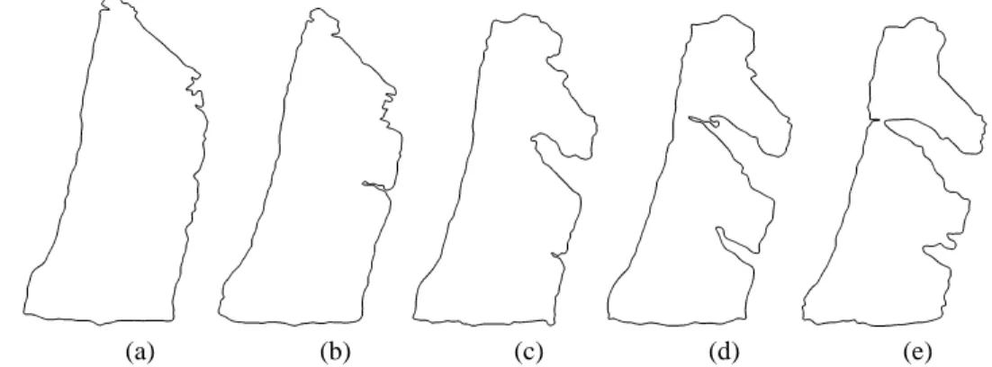
An excellent example of wave erosion and its accelerated effects at local surface

irregularities is given by Robe et al. (1976, 1977) in their report of a series of 5 full-scale aerial observations made by the IIP of an large tabular iceberg on the Grand Banks over a period of 25 days from May 12 to June 6, 1976. It was last sighted at 47°31’ N, 49°07’W after having drifted across the northern entrance to the Flemish Pass. The iceberg had only 4m to 5m of freeboard and was very stable. A plot of surface area over the 25 days showed a nearly linear decrease in surface area from an initial 190,000 m3 to 109,000 m3. The rapid deterioration was due primarily to wave induced erosion with associated undercutting and minor calving. Surface water

temperature was reported to be between 2°C and 4°C and the water temperature at about 75m to 100m was estimated to be a minimum of less than -1°C.

The visual record gives clear evidence of localized accelerated wave erosion at points around the perimeter that appear to have some initial surface irregularity. The authors concluded that a concentration of wave energy and local turbulence at these points led to progressive enlargement of small embayments. The bottom of these embayments appear to have extended only several meters below the water surface and were parallel to the water surface. The shape of the bottom of the iceberg was assumed to be flat.

The authors noted that such observations are very rare as icebergs usually change appearance rapidly due to calving, rolling, and melting so that repeated identification of the same iceberg is impossible even after a few days.

(a) (b) (c) (d) (e)

Note that when icebergs are in pack ice, they are protected from wave erosion by the pack, which dampens wave motion. Bergs undergo more rapid wave erosion in the open sea (e.g Marko 1996).

3.3 Fragmentation Processes 3.3.1 Global cracking

The topic of natural and artificial splitting of icebergs was addressed in Diemand et al. (1987). The authors considered 4 sources for the stresses in icebergs (with estimated levels);

1. residual stress (remnant from glacial deformations) (≈0.1 MPa - widespread) 2. hydrostatic stresses (from the surrounding water) (small - widespread)

3. thermal stresses (arising from the heat transfer during melting) (up to 2 MPa - local) 4. buoyancy stresses on the projecting underwater rams. (≈0.5 MPa - local)

The level of residual stresses could vary widely. Stresses in glaciers are sufficient to deform the ice, although at very small strain rates. A proper estimate of the residual stresses should take the creep behavior of ice into account. In time, the residual stresses would likely all dissipate. This issue would be well served by field observations. There are methods for establishing the level of residual stresses experimentally. Whether this can be practically accomplished on an iceberg should be studied.

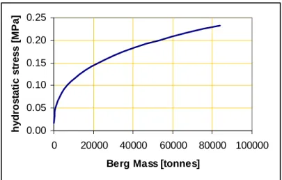
The hydrostatic stresses can easily be estimated. Figure 6 shows the hydrostatic stress on the base of a blocky berg (1 : 1.5 : 2) versus iceberg mass. Stresses of the order of 0.1 to 0.3 MPa are easy to achieve. These are, of course, the same stresses associated with buoyancy, although the buoyancy stresses referred to in item 4 above are actually bending stresses arising from

0.00 0.05 0.10 0.15 0.20 0.25 0 20000 40000 60000 80000 100000

Berg Mass [tonnes]

hy dros ta ti c s tr e s s [ M P a ]

Figure 6. Maximum hydrostatic stress versus iceberg mass (assumes a 1:1.5:2 block).

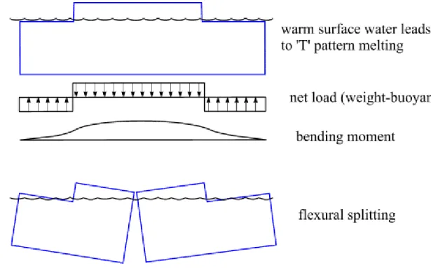
One particular mechanism was postulated to explain the large fragmentation events often observed. The authors described tabular icebergs that split roughly in half. Figure 7 shows the mechanism proposed by Diemand et al.(1987). The relatively warm surface temperatures in the Labrador Sea in summer was postulated as the cause of enhanced waterline melting leading to the development of large underwater rams (see Figure 7). In such circumstances, bergs have been observed to split in the center with the central region of the iceberg sinking as the ends tilt up. The mechanism is a simple bending failure, in which tensile stresses exceed a limit, resulting in fracture. For the case of a particular berg, an 8 million tonne berg called Gladys, tensile stresses of 0.8MPa were estimated.

Diemand et al. made simple estimates of iceberg mechanical strength on the basis of grain size and strain rate. Quoting Lee and Schulson (1986) for a strain rate of 10-7 s-1, and -10° C , a strength versus grain size equation is given as

5 0. od K − = σ (15)

where Ko is 0.05 MPa√m. For an assumed grain size of 7.3 mm, a strength of 0.6 MPa is found,

Figure 7. Tabular iceberg splitting in flexure (after Diemand et al. 1987).

3.3.2 Time dependent strength

The primary stresses on icebergs are sustained over a very long time, whether it be gravity, buoyancy or thermal in origin. Some stresses would be short lived, such as those due to bottom impact, wave impact or the inertial and hydrodynamic forces occurring during a roll-over event. The duration of the stress is quite important. Ice strength is a time-dependent property.

"The absolute values of ice strength, as well as the magnitudes 2of the ice strength parameters change from the greatest (instantaneous) values at the time of loading (to)

to zero for longer intervals." (Fish 1991)

In order to understand natural fragmentation processes, one must consider time dependent strength. (Note: this time dependency helps to explain why various methods to fragment ice rapidly, including the use of explosives, have tended not to work. Sustained stresses are much more effective at causing large fractures in ice.)

There are several time dependent ice strength models. Fish (1991) describes a creep model for ice strength that uses a parabolic strength model with time dependent parameters. The model assumes positive compressive stresses (i.e. may not be suitable for tensile or flexural stresses). For constant stress conditions, the shear stress at failure τi is given as

2 m max m i

)

t

(

b

)

t

(

b

)

t

(

c

)

t

(

σ

σ

σ

τ

=

+

⋅

−

⋅

where c(t) and b(t) = tan φ (t) are the cohesion and friction angle, and σm is the mean normal stress

3

σ

σ

σ

σ

=

+

+

where σ1 ,σ2 ,σ3 are the principal stresses. For relatively low confining stress, the failure criterion becomes

m

i t c t b t σ

τ ( )= ( )+ ( )⋅ (18)

At very low stress or strain levels, as we would have in long-term iceberg failure processes, such as natural splitting and spalling, but not collision, Fish states that strength becomes independent of confining pressure, so that we have a simple shear strength (cohesion) criterion:

) ( ) (t c t i = τ (19)

Fish further states that the time dependency can be included as

) ( ) (t c_o t i = ⋅Φ τ (20) where n o t t t / 1 ) ( −     = Φ (21)

n is a parameter in the range of 3 to 5, and to is a time parameter equal to the lower limit of

validity of creep behaviour. Fish suggests a upper strain rate limit of

ε

&

=

sec 01 . 0 2000 1 = = ε& o t (22)

Fish reported data from (Jones 1982) for polycrystalline ice at -12°C. The exponent n =3.95 and co = 16.4 MPa. With this a time dependent shear strength equation (for low confining positive

pressures, sustained stresses) becomes

( )

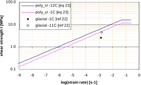
With time plotted in days, Figure 8 shows the declining shear strength with time. This curve is specific to the data by Jones, but is representative of the type of ice and temperatures in icebergs. The same data is plotted as strength versus strain rate in Figure 9.

0.10 1 10 100 0.00000001 0.000001 0.0001 0.01 1.0 100. Time [days] St re n g th [ M Pa ] co to c(t) c(t)= c (t)oΦ c = 16.4 o MPa, to= .01 s Φ(t) = (t/t ) , o -1/ n n = 3.9 5

Figure 8. Time dependent shear strength for polycrystalline ice at -12°C.

0.1 1.0 10.0 100.0 -9 -8 -7 -6 -5 -4 -3 -2 -1 0 log(strain rate) [s-1] sh ear s tr e n g th t [ M P a ] poly_cr -12C [eq 23] poly_cr -1C [eq 23] glacial -1C [ref 22] glacial -11C [ref 22]

Figure 9. Shear strength versus strain rate for polycrystalline ice at -1°C, -12°C for equation 23, and data from Gagnon & Gammon (1995b).

3.3.3 Thermal cracking

Despite the relatively minor role of melting due to solar radiation, thermal stress fluctuations, which will be most severe in the above water part of an iceberg, may induce cracking,

particularly local surface cracking. This ablation mechanism has received very little attention in the literature, although Robe (1980) pointed out anecdotal reports of increased cracking and calving activity coinciding with sudden increases in the amount of radiation, such as occurs on sunny mornings.

3.4 Deterioration models

Several deterioration models have been described in the literature. The most prominent are those from the International Ice Patrol (Anderson 1983) and El-Tahan et al. (1984), which are aimed at complementing drift models.

The IIP deterioration model (Anderson 1983) is based entirely on work done by White et al. (1980) and includes four deterioration mechanisms: insolation, buoyant natural convection, underwater forced convection, and wave erosion. Air convection and fragmentation processes, including calving due to wave erosion are ignored. Using the model, the sum of the deterioration components are summed and the total deterioration is calculated as a percentage of the starting size of an iceberg. As IIP usually does not collect any detailed information on iceberg size or geometry, but rather only on approximate size classification (i.e. growler, small, medium, large), the starting lengths are somewhat arbitrarily assigned lengths that are deemed to be characteristic of the iceberg’s estimated size class. Clearly, the purpose of the model is to make gross estimates of the expected change in size of a multitude of iceberg targets, rather than give anything

approaching a detailed account of a particular iceberg’s evolution.

Hanson (1988) explained that the IIP parametric forecast model of iceberg deterioration, in conjunction with its dynamic drift model (Mountain 1980), is used to complement their primary role in identifying iceberg threats by helping to establish positive iceberg resights and to

eliminate targeted icebergs from their forecasted drift. This is especially important when

intervals between observations are long. The author reported a field study that was undertaken to critique the IIP deterioration model, with particular emphasis on checking the accuracy of

environmental input data. This work illustrates the importance of accurate input data.

Six medium icebergs were observed by ship for up to 6 days near 50°45’N 53°30’W. In situ environmental data were collected and the IIP model was used to make predictions using both the its normal ’global’ environmental inputs and the in situ data. Based on a comparison of the results Hanson concluded that while the modeled insolation was likely to be off by 100%, the relative insignificance of this component and the difficulty of acquiring and incorporating detailed insolation data in the model was not worthwhile. Likewise, the effect of using surface water temperature in the model was compared with using more precise water temperature

measurements at depth. Using surface temperature was found likely to result in overestimation of both buoyant and forced convection by a factor of about 3. This error would only occur in

summer when the sea temperature was warm enough to cause melting. Unfortunately, the author says that deeper water temperatures are not easy to get and the status quo is good enough. With

respect to forced convection in terms of the effect of the relative motion between the iceberg and water, the IIP model use of historical current data to judge water speed, and its neglect of wind driven current was found to lead to significant error that could be put right by incorporating wind driven current, which is used in the drift model. The most important component in the model, wave erosion, was found to be over predicted by the IIP model because of the global wave data inputs were over predicted. This could be addressed by using better wave climate prediction models.

Very little is reported about the actual iceberg observations. While the observation period was not long, the presence of growlers and bergy bits near the icebergs indicated that they were in a state of rapid deterioration. One iceberg was observed to roll over, which resulted in its height doubling and its waterline length increasing by about 5%. Changes in the above water shape of several other icebergs indicated that they too had rolled, although they were not observed doing so. Remarkably, the author made no recommendations that fragmentation processes be modeled in future.

El-Tahan et al. (1984) provide a detailed account of their iceberg deterioration model, which derives strongly from White et al. (1980) and has been used in a series of subsequent

publications, some of which are discussed below. The model is exercised for three cases and comparisons are made with corresponding field observations. Two of the field observations (Kollmeyer 1965 and Robe et al. 1977) are in the open literature, the third is not. The authors show that wave erosion and calving associated with wave erosion is the most important

deterioration mechanism, accounting for more than 80% of the mass loss. Melting due to forced convection is significant at about 16%, which is about 8 times the melting rate due to natural buoyant convective melting. Insolation and wind convection account for less than 0.5% each. The authors say that underwater fragmentation of shelves, accelerated erosion and cracking at flaws, and thermal stress cracking are practically impossible to model and these omissions might explain differences between observed and predicted deterioration.

Venkatesh et al. (1985) reported results from a detailed 15 day field study of 2 grounded bergs (1.6×106 and 0.8×106 tonnes) off St. John’s. The fact that the icebergs were grounded close to shore made local measurements of environmental conditions and observations of local

deterioration practical, which is not often the case. A comparison with an iceberg deterioration model (El-Tahan et al. 1984) was made and found to underestimate mass losses by about 10% in one case, and substantially more in the second case. The authors attributed the relatively poor comparison in the second case to difficulties associated with the change in iceberg orientation during the observation period, which they claimed introduced errors in estimates of mass

Another suggested reason for the poor comparison was that other mass loss mechanisms that were not modeled, such as thermal cracking, caused more rapid deterioration than predicted. In the first case, the model indicated that 88% of the mass loss was due to wave erosion and the associated calving from overhangs, 9% due to forced water convection, 2% due to buoyant convection, and 0.5% each due to wind convection and insolation. The authors also provided a brief review of previous deterioration work, going back to 1912.

Venkatesh (1986) picked up one of the loose threads from Venkatesh et al. (1985) by pursuing an explanation of the poor comparison between modeled and observed results of the deterioration of a 0.8×106 tonne iceberg, the second of the two icebergs studied previously. Consideration is given to how grounding might affect estimates of iceberg mass and

deterioration rate, especially in light of the reorientation of the observed iceberg, although the results do not add significantly to the original paper.

Venkatesh and El-Tahan (1988) undertook work to determine how melting affected iceberg distributions. This is similar in intent to the IIP’s use of a deterioration model, although the authors apply a more detailed characterization of icebergs by category than do the IIP.

Venkatesh et al. (1994) exercised El-Tahan et al.’s (1984) deterioration model in connection with a field study of iceberg drift in sea ice. The main aim of the field work was to investigate the effect of sea ice on iceberg drift for IIP drift model validation, although Mountain’s (1980) model does not contain a sea ice force term. To do so, two medium tabular icebergs were

instrumented and tracked using satellites for more than a month in the marginal ice zone at about 51° to 52°N offshore Newfoundland and Labrador. The ice concentration was about 9/10s at the start of the field work and changed to 3/10s before the work was complete. Interestingly, the drift model seemed to do as well in broken sea ice as in open water, indicating that broken ice, even in high concentration, does not have a large impact on drift. In terms of deterioration, the remote location of the icebergs precluded anything approaching continuous observation of local deterioration processes, so the comparison of predicted with actual results requires a certain amount of inference. The temperature and wave height inputs, which are important in the dominant wave erosion and calving deterioration terms, were based on reasonable estimates, although not always direct measurements on site.

3.5 Iceberg shape

Icebergs evolve into unusual shapes that defy simple categorization, although the size and shape categories that have been defined by the IIP and the World Meteorological Organization (1970) are widely used for descriptive purposes.

Three size categories are given by the WMO: icebergs, bergy bits, and growlers. An iceberg is defined as a massive piece of glacial ice whose above water volume, or sail, extends at least 5 m above the waterline and has a water plane area greater than 300 m2. The sail of a bergy bit extends between 1 m and 5 m above the waterline and has a water plane area of about 100 to 300 m2. The smallest size category is growler and this refers to a piece of glacial ice that extends less than 1 m above the waterline and has a water plane area of about 20 m2.

The IIP size categories shown in Table 5 are roughly the same, but they further divide the iceberg category into small, medium, large, and extra large sizes. IIP size and shape

classifications have changed over the years in response to detection methods.

Table 5. IIP iceberg size categories (IIP website). Category Height [m] Length [m]

Growler < 1 < 5 Bergy Bit 1-4 5-14 Small 5-15 15-60 Medium 16-45 61-122 Large 46-75 123-213 Very Large > 75 > 213

The IIP also has shape categories: tabular and non tabular. Non tabular shapes include blocky, pinnacle, dry dock and dome. Tabular icebergs have horizontal or flat tops with a maximum waterline length to sail height ratio greater than 5:1. The largest icebergs are tabular. Blocky icebergs are steep sided and flat topped with a length to height ratio of about 2.5:1. Pinnacle icebergs are characterized by a central spire or a pyramid shape that may have several spires. Drydock icebergs have a wave eroded U-shaped slot between two or more columns or pinnacles. Dome icebergs are smooth and rounded with low sides (e.g. Robe 1980). Venkatesh & El-Tahan (1988) added estimates of perimeter, mass, and surface area to average size classifications as shown in Table 6.

Table 6. Average iceberg size (after Venkatesh & El-Tahan 1988). Category Length [m] Mass (tonnes) Perimeter [m] Wetted surface area [m2] Total surface area [m2]

Growler (non tabular) 10 450 30 250 350

Small (non tabular) 55 75,000 155 8,000 10,300

Medium (non tabular) 125 900,000 360 36,000 48,000

Large (non tabular) 225 5,500,000 650 110,000 150,000

Small (tabular) 80 250,000 235 15,000 20,000

Medium (tabular) 175 2,170,000 500 67,000 92,000

Large (tabular) 260 8,230,000 750 150,000 204,000

A number of field studies of iceberg size, shape, and other characteristics have been carried out over the years on the Grand Banks and Labrador Sea, many in connection with oil and gas industry activities. A recent report (Anon. 1999), sponsored by the Program for Energy Research and Development (PERD), has compiled much of the information from over 40 reviewed

reports, including data that has previously been confidential, into a single database. The main aim of the compilation effort was to get a better idea of iceberg shape in order to better inform the estimation of iceberg impact loads for offshore installation design. The database includes dimensions for 872 icebergs, detailed 3-dimensional sonar profile information on the underwater portion of 28 icebergs, detailed 3-dimensional information on 566 iceberg sails from stereo photography, and 2-dimensional profiles of 155 iceberg sails and keels. This is a very useful source of field measurements and complements the iceberg sightings statistics reported by Singh et al. (1998). The authors also did a simple analysis of the length, width, height, draft, and mass data that they compiled, and reported results such as length versus draft relationships. Some earlier attempts to find meaningful relationships between above water parameters and draft were not successful (e.g. Buckley et al. 1985).

The database contains significantly more 3-d above water iceberg data (from stereo pictures) than 3-d underwater data (sonar profiles). The authors make the bold assumption that the above and under water shapes are statistically similar, based on the premise that icebergs roll

frequently, although this is not justified by the authors. Such an assumption cannot go unchallenged and should be addressed.

In a subsequent study, some of the 3D data were compiled into a visualization database (Barker et al. 1999). This included 52 sail and 25 keels. In only 3 cases were both sail and keel data available.

3.5.1 Shape definition

The choice of method of representing the natural surfaces of icebergs is directed by the need for flexibility to describe the shape, keep track of and update shape changes, determine hydrostatic, floatation, and stability characteristics, and evaluate stresses.

Right handed Cartesian coordinate systems are used here. A set of inertial, or space axes, denoted xo, yo, zo is fixed with respect to the undisturbed water surface with the zo axis pointed

down. A non inertial, or body, axes system x, y, z is fixed to the iceberg body. As the iceberg shape evolves, the axes will reorient itself with the iceberg as it moves to maintain static equilibrium, but its initial origin position can be chosen for convenience. The position and orientation of the body axes with respect to the space axes is given by the Cartesian coordinates (xo, yo, zo) measured in the direction of the xo, yo, zo axes, respectively, and by the Eulerian angles

(Φ,Θ,Ψ). For example, the position of the origin O of the iceberg body axes with respect to the inertial system is

{

}

where the right hand side is the column matrix representation of the vector, as indicated by the transpose T.

The surface is defined by a series of points (x, y, z) in the body system and a surface unit normal vector nˆ into the body at each point. Each surface point is explicitly associated with two nearby points to form a triangular surface plane: unit tangents from the surface point to its two associated points define the surface normal. The set of elemental triangular areas constitute the discretized surface area. Changes in shape due to continuous ablation processes are evaluated at each point at specified time intervals; likewise the surface normals are evaluated at each point using the new positions of the surface points. As the ablation processes involve a variety of environmental conditions that are more or less directional, it is necessary that the vectors defined in the body system be known in the inertial system as well. This can be done with the appropriate coordinate system transformation, which is described in detailed below.

The surface geometry representation described above is robust and easily adaptable to several software platforms. The initial geometry must be explicitly defined and subsequent continuous changes can be handled automatically. Discrete fragmentation events and the resulting geometry changes are handled separately.